Commitment and (in) Efficiency: A Bargaining Experiment

ABSTRACT

In many matching markets, bargaining determines who matches with whom and on what terms. We experimentally investigate allocative efficiency and how subjects’ payoffs depend on their matching opportunities in such markets. We consider three simple markets. There are no information asymmetries, subjects are patient, and a perfectly equitable outcome is both feasible and efficient. Efficient perfect equilibria of the corresponding bargaining game exist, but are increasingly complicated to sustain across the three markets. Consistent with the predictions of simple (Markov perfect) equilibria, we find considerable mismatch in two of the markets. Mismatch is reduced but remains substantial when we change the nature of bargaining by moving from a structured experimental protocol to permitting free-form negotiations, and when we allow players to renege on their agreements. Our results suggest that mismatch is driven by players correctly anticipating that they might lose their strong bargaining positions, and by players in weak bargaining positions demanding equitable payoffs.

1. Introduction

A fundamental question in economics is whether the “right” people end up in the “right” jobs. Labor markets are important and their allocative efficiency is crucial for the productivity of the economy. The typical way that frictions have been modeled is through costly search and imperfect information.¹ However, in many high-skill labor markets, these frictions are limited. Workers typically know which firms are looking to hire, and similarly firms know which workers would be appropriate for a given vacancy. Does this mean that the right workers will end up in the right firms? More specifically, absent these frictions, can decentralized bargaining be expected to result in an efficient allocation of workers to firms?

On the one hand, if the aforementioned frictions are absent, then in line with a Coasian logic it might be hoped that two parties leave no gains from trade on the table when bargaining. If so, and this holds across all possible worker–firm pairs that could match, then by results from Shapley and Shubik (1972), the matching market will clear efficiently.

On the other hand, agreements in decentralized matching markets are typically reached sequentially, causing the composition of the market to change over time. As this market context evolves so can the bargaining positions of those remaining in it. Suppose it is efficient for a worker, Ann, to match to a firm, B, but that Ann is currently in a strong negotiating position; there is another firm, C, with a vacancy Ann could instead fill. Although Ann would be less productive with firm C, Ann would still like to use this alternative possible match to bid up her wage with firm B. However, this alternative vacancy at C might be filled by someone else, in which case Ann would lose her strong bargaining position. Indeed, if there is no chance Ann will match inefficiently with firm C, then firm B might as well wait for C’s vacancy to be filled and for Ann’s bargaining position to deteriorate. Can agents who find themselves in temporarily strong bargaining positions benefit from these positions without sometimes matching inefficiently?

No empirical work we are aware of investigates whether bargaining frictions, that is, the strategic actions of market participants to improve their terms of trade, can lead to allocative inefficiency. Fundamental identification problems inhibit such an investigation. Even under very strong assumptions it is hard to identify whether matches are positively or negatively assortative from wage data (Eeckhout and Kircher 2011).² More generally, to observe the extent of mismatch, an econometrician must estimate the counterfactual productivities of matching different people to different jobs. But unobservable worker characteristics that are valued differently by different firms can generate any counterfactual productivities and rationalize any given match as efficient. Even if it is possible to detect inefficient matches, it would be hard to separate the role of bargaining frictions and other frictions. To overcome these problems, and provide some first empirical evidence on bargaining frictions, as opposed to search or informational frictions, we take an experimental approach.

We use laboratory experiments to study how payoffs are affected by the structure of the market and whether allocative efficiency, matching the “right” worker to the “right” job, is achieved by decentralized bargaining. Matching is one-to-one, and we consider the simplest markets in which a player can lose a matching possibility as others reach an agreement and exit. Our experiments feature two characteristics, which are common in many labor markets: heterogeneous match surpluses and endogenous agreements regarding how the surplus generated by a match is split.³ In the laboratory, we control the entire set of possible match surpluses, removing unobserved heterogeneity in match quality and observing counterfactual match productivities. We also track individuals’ bargaining patterns in full.

In our main experiment, Experiment I, we use a standard bargaining protocol from the theoretical literature to study three simple markets. In all three markets, there are two players on each side of the market, and on each side of the market, one player is in a strong bargaining position, whereas the other is in a weak bargaining position—the weak worker is only a good fit for the strong firm and the weak firm can only productively employ the strong worker, whereas the strong worker and strong firm can also productively match with each other, causing the weak buyer and weak seller to be left unmatched. It is always efficient for the strong worker to match to the weak firm and the weak worker to match to the strong firm. The three markets vary only by the value of the surplus the strong worker and strong firm can obtain by matching with each other.

These markets are designed so that increasingly complex strategies in the corresponding noncooperative game are required to reach an efficient outcome. As more complicated strategies are required, we find increasing rates of mismatch. The rates of inefficient matching are substantial, increasing from 0% to 49% to 70% across the three treatments. Players in strong bargaining positions, with alternative possible matches, are able to exploit these bargaining positions and receive higher payoffs as the value of their alternative (inefficient) match increases. We also find that the market composition at the time agreements are reached matters. Once strong participants’ alternative possible matches have been lost, they receive a lower payoff.

The Markov perfect equilibria (MPE) organize our data very well across a number of dimensions, including comparisons across the three markets of efficiency and the payoffs of players in strong and weak bargaining positions. The essential logic of the MPE predictions is that players in strong bargaining positions match inefficiently because they correctly anticipate the possibility that they might lose their strong bargaining position. The main discrepancy between the data and MPE predictions is that there is more mismatch than predicted. An explanation for this, which is consistent with our analysis of players’ strategies, is that players sometimes demand at least equitable payoffs. For players in strong positions, this constraint is nonbinding, but for weak players it means that, in comparison to the MPE, they ask for too much when making offers and reject offers they should accept. Whereas in the ultimatum game players playing in this way induce others to make more equitable offers, in our market setting, our results suggest that it leads players in strong positions to inefficiently match with each other, thereby excluding weak players and leading to both less equitable outcome and more mismatch than predicted by the MPE.

An important question concerning our findings, especially when considering their external validity, is: What features of our environment drive the inefficiency we find? Two features, in particular, merit a closer examination. The first is our bargaining protocol, which constrains the interactions among our participants. This creates artificial frictions that could be responsible for the inefficiencies we document—in practice, interactions in markets are much less constrained than in our experimental protocol, or in fact any protocol corresponding to a dynamic bargaining model from the theoretical literature. Second, our experiment endows players with commitment power—after an agreement is reached, players are unable to renege on it. As whenever an inefficient outcome is obtained, there exist at least two players both of which could do better by instead matching with each other; this commitment power seems likely to be important. However, unlike the constraints on interactions imposed by the bargaining protocol, this is a feature that seems to be present in many matching markets. Firms, and to a large degree also workers, rarely renege on agreements they have reached.

In Experiments II and III, we investigate these two explanations. In Experiment II, we let participants interact in an unstructured way, allowing them to make and remove offers to anyone at any time. The market composition at the time agreements are reached continues to affect the terms of trade, and although the rate of mismatch is reduced, substantial inefficiencies remain. In Experiment III, we instead adjust the bargaining protocol to let participants renege on agreements they have reached at a small cost. This reduces inefficiencies a bit more than removing the protocol, but again inefficiencies remain.

We contend that in many real labor markets the bargaining positions of players change as others reach agreements and exit the market. Our experimental investigation replicates and studies this feature. Alternative matches affect the average terms of trade agreed upon. The composition of the market, which workers and which firms are still searching for a match, thus matters, and players’ bargaining positions are nonstationary. Evidence across our three experiments collectively suggests that this nonstationarity is intimately tied to high rates of inefficient matching. Our experiments provide some first evidence for the role of bargaining frictions, as opposed to search or informational frictions, in decentralized matching markets.

Finally, before we dive into our investigation, we want to step back and address concerns regarding the general ability of laboratory experiments to obtain results that can be generalized to real markets. This is an important question as the ultimate goal of our investigation is to obtain qualitative insights that inform us about the world outside the laboratory.⁴ Our paper joins the branch of experimental literature termed theory-based experiments.⁵ The philosophy behind theory-based experiments is to capture key aspects of real economic environments in simplified settings, and to observe real subjects making decisions with monetary consequences. This can enable clean tests of important workhorse theories, and speak to important economic outcomes, which can be very hard to test using field data. In general, the impediments to such field data examinations include the scarcity of data, unobservability of counterfactuals, endogeneity problems, and other confounding factors that prevent identifying causal effects. The very complexity and existence of these confounds in naturally occurring data is precisely why controlled laboratory tests provide a valuable additional source of data. If the theoretical predictions fail in the simplest and most transparent applications of the model, then that casts serious doubt on the usefulness of the theory when applied to more complex settings. Furthermore, the data created from carefully controlled settings can be used toward the development of better theoretical models.

Related Literature.

We focus in this section on the related experimental literature. We discuss the theoretical literature in the context of our different experimental protocols.

There is a large experimental literature on bargaining.⁶ The most relevant to our paper is the study by Binmore, Shaked, and Sutton (1989), which investigates the effect of exogenous outside options on the bargaining position of players in a two-person bargaining setup that has features of both the alternating-offer and ultimatum-game protocols. The authors find that responders receive a payoff equal to their binding outside option, providing support for the “outside option principle”.

Our paper is also related to the experimental literature on decentralized two-sided matching markets, which is relatively thin and for the most part focuses on matching markets with nontransferable utility (NTU). The prominent studies in this space include Echenique and Yariv (2013) and Pais and Veszteg (2011). Echenique and Yariv (2013) consider fully decentralized two-sided matching markets with complete information and find that most markets reach stable outcomes. When more than one stable outcome exists, the outcomes gravitate towards the median stable match. Pais and Veszteg (2011) study both complete and incomplete information matching markets and vary search costs and the degree of commitment to formed matches; this last variation is similar to us allowing players to renege on their agreements, which we do in our Experiment III. The authors find that in complete information markets, which are the closest to our setup, the degree of commitment affects both the frequency of efficient final matchings and the level of market activity as captured by the number of match offers made by subjects. Contrary to our main finding, the authors document that the treatments with commitment correspond to the highest proportion of efficient final outcomes.⁷

The main difference between our paper and those discussed previously is that we allow bargaining over the terms of trade, studying decentralized matching markets with transferable utility (TU). This brings to light an additional dimension of the bargaining process that is missing, by construction, from games with NTU: Bargainers need to agree not only on who is matched with whom but also on how to split the available surplus between the pair of potential match partners. The only other experimental study of decentralized matching markets with TU that we are aware of is the study by Nalbantian and Schotter (1995). In this paper, the authors analyze several procedures for matching with players who are privately informed about their payoffs.⁸ The authors find that although efficiency levels were relatively high in all treatments, different mechanisms suffered from different types of problems: Some produced a considerable number of no-matches, whereas others produce a substantial number of suboptimal matches.

There is a small experimental literature studying bargaining on networks, which is surveyed in Choi, Gallo, and Kariv (2016). The study most closely related to ours is Charness, Corominas-Bosch, and Fréchette (2007), which examines experimentally the effects of network structure on market outcomes following the model of Corominas-Bosch (2004). The bargaining is structured as a sequential alternating public-offer bargaining game over the shrinking value of homogeneous and indivisible goods. Offers made by players on one side of the market alternate with offers made by players on the other side of the market, and all players on a given side of the market make offers simultaneously. An offer is a price that is announced to all players on the other side of the market, who then choose which offers to accept. Experimental results qualitatively support the theoretical predictions and display a high degree of efficiency: Total payoffs of players constitute over 95% of the maximum attainable surplus, and three-quarters of all agreements are reached in the first bargaining round.⁹

Finally, there is an experimental literature in sociology that studies how network structures confer power. Two foundational papers are Cook and Emerson (1978) and Cook et al. (1983), and there is a nice albeit brief discussion in Jackson (2010). A typical experimental design in this literature has several features different from us, and more importantly, the focus is on identifying strong and weak network positions rather than evaluating the efficiency of markets. As far as we are aware, this literature does not investigate the interaction between changing market composition and efficiency, and the typical protocol considered does not lend itself to such an investigation by preventing players from exiting before negotiations among all possible matches have taken place.¹⁰

2. Environment

2.1. Basic Setup

We set out to test whether the endogenous evolution of thin, heterogeneous matching markets can result in an inefficient allocation of workers to firms in the case of labor markets, buyers to sellers in product markets, or men to women in the marriage market. As we suspect that inefficiencies will be more likely in more complicated settings, we consider the simplest possible markets capable of exhibiting the effects we are interested in. For bargaining positions to change as others exit, we need the market to be able to support at least two matches, requiring at least four players, and at least three different matches among these four players to be possible.

Figure 1 presents three different market structures (Game 15, Game 25, and Game 30), which will serve as the basis of our investigation. These are four-person markets, with each player identified by the letter A, B, C, or D. A link between two players indicates the joint surplus that this pair of players generate by matching with each other, with the surplus indicated by a number next to the link. These are one-to-one matching markets, that is, each player can be matched with at most one other player in the market. The payoffs of unmatched players are normalized to 0. In all three markets, the vertical links (the link between A and C and the link between B and D) generate a surplus of 20 units. The markets differ in one feature only: the value of the diagonal link between A and D. In Game 15, this link is worth 15 units, in Game 25, it is worth 25 units, and in Game 30, it is worth 30 units. This diagonal link determines the bargaining position of A and D vis-á-vis C and B. We will refer to A and D as the strong players, and to B and C as the weak players. In all three markets, it is efficient for A and C to match and for B and D to match. Across these three markets, we study how the average payoffs of players differ and the frequency with which the efficient match is reached.

Figure 1.

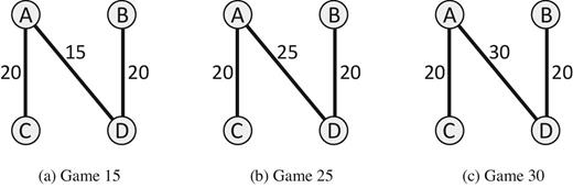
The three markets considered in this study. We refer to players A and D as the strong players and players B and C as the weak players.

2.2. Key Issues and Experimental Approach

There are several fundamental questions we hope to address through our experiments.

Efficiency.

First and foremost, when can decentralized bargaining in matching markets be expected to efficiently match the two sides of the market? What are the mechanisms that facilitate efficient matches being reached? What causes inefficient outcomes?

Network Bargaining Power.

How do players’ network positions affect their payoffs? Can players with alternative matching opportunities play these alternatives off against each other to extract most of the rents? Does the possibility that these alternative matching opportunities will be lost limit the extent to which agents can exploit strong network positions?

To explore these questions, we focus mainly on an experimental protocol that mirrors a standard noncooperative bargaining game (Experiment I). There are competing theories that offer different predictions about both efficiency and network bargaining power. A general finding from the noncooperative bargaining literature is that there is a tension between using simple strategies and using strategies that can sustain efficient outcomes. An advantage of using this protocol is that the corresponding noncooperative game is tractable, and we can cleanly test how this trade-off between complexity and efficiency is resolved. Better understanding this can inform us about what insights regarding efficiency and network bargaining power from the theoretical literature are most applicable in different situations.

However, it is also important to understand the limitations of this approach. In particular, there are two key features of the bargaining environment in Experiment I we would like to understand better. First, how important is the rigid bargaining protocol? Does it prevent players from achieving efficient outcomes by limiting the interactions between them, or aid efficiency by limiting the extent to which players can try to manipulate each other? Second, in the bargaining protocol of Experiment I, agents leave the market after reaching an agreement. Thus, players are endowed with commitment power by the protocol—they commit not to renege on an agreement whenever they reach one. Does removing this commitment power and allowing players to renege on agreements increase or reduce efficiency? On the one hand, commitment is often useful in a variety of settings for achieving efficient outcomes. On the other hand, it makes the environment less stationary and more complicated. We conduct two additional experiments. In Experiment II, we remove the experimental protocol and allow players to make offers to whom they want and when they want. Hence, we investigate the role the protocol plays in our Experiment I results. In Experiment III, we follow a structured protocol similar to Experiment I, but with the exception that players remain in the market after they have reached an agreement and can renege on that agreement at a small cost. Hence, we investigate the role of commitment in our Experiment I results.

3. Experiment I: Theory

To guide our experimental investigation, it is helpful to consider some alternative theories. These theories yield different predictions of players’ expected payoffs and matches—and, thus, the level of efficiency in the market. For each theory, we briefly describe the main idea and implications for the three games depicted in Figure 1. We refer the reader to Appendices  A,  B, and  C for additional details.

The experimental protocol we consider is standard and extends Rubinstein bargaining to accommodate many players. The corresponding game has an infinite horizon with a common discount factor δ ∈ (0, 1). In round t, there is a set of unmatched players who are active. One player is chosen uniformly at random to be a proposer. If the proposer is already matched, we move to round t + 1; otherwise, the proposer can choose to propose a match or to do nothing. To propose a match, the proposer must select an unmatched player and suggest a division of the surplus their match would generate. If a proposal is made, then the player who receives the proposal must either accept or reject it. If the proposal is accepted, then a match is formed, and those two players, having reached an agreement, leave the market. If the proposal is rejected, then both players remain unmatched and we move to round t + 1. The game ends when there is no positive surplus between any two unmatched players.

Although there will often be multiple equilibria of this dynamic game, following the literature, we focus on two criteria on which equilibrium selection can be based—simplicity and efficiency. Simplicity has led a large literature to study the MPE of related bargaining problems, including Rubinstein and Wolinsky (1985), Rubinstein and Wolinsky (1990), Gale (1987), Chatterjee and Sabourian (2000), Sabourian (2004), Gale and Sabourian (2006), Polanski and Winter (2010), Abreu and Manea (2012b), and Elliott and Nava (2019). In our context, the MPE are perfect equilibria in which players choose strategies that depend only on which other players remain active in the market, rather than on the entire history of play.¹¹ Although this prevents players from having to keep track of complicated histories of play, it limits the ability of players to punish and reward each other. When there are no efficient MPE, a natural question that then arises is whether more complicated strategies could obtain efficient outcomes. A second type of equilibria we will consider are efficient perfect equilibria (EPE). By design, the markets we study require increasingly complex strategies for an efficient perfect equilibrium. In Game 15, there is an efficient MPE. In Game 25, there is no efficient MPE, but there is an EPE that punishes deviations by reverting to the MPE. In Game 30, there is no efficient MPE or EPE that relies on Markov reversion, but there is an EPE that relies on more complicated strategies. Thus, as we move from Game 15 to Game 25 to Game 30, ever more complicated equilibrium strategies are required to obtain the efficient outcome.

3.1. Quantitative Theoretical Predictions

We begin by describing the limit MPE payoffs and provide some intuition for Games 15, 25, and 30. In all these games, there is a unique MPE. In Game 15, all players always proposing efficiently is an MPE. When all players do so, it is as if they bargain bilaterally with their efficient partner and all players receive limit payoffs of 10. Given that offers of less than 10 will be rejected, it is unprofitable for A or D to deviate and instead offer to each other. Thus, in Game 15, the efficient match is reached with probability 1.

In Game 25, it is no longer an equilibrium for only efficient offers to be made. If A and D never use their link, they will get limit payoffs of 10 as before, but now they will have a profitable deviation to instead offer to each other when selected as the proposer. In equilibrium, A and D mix between offering to each other and making efficient offers. Whenever A and D match with each other, players C and B get a payoff of 0. This reduces the amount players C and B are willing to accept when they do receive offers. In Game 25, the efficient match is obtained when C or B propose, but not always when A or D propose. Given the equilibrium probability with which A and D offer to each other, the probability the efficient match is reached is 0.72.

As the value of the diagonal link increases to 30, we reach a corner solution in which A and D can no longer push down the expected payoffs of C and B enough for them to be indifferent about whom to offer to. Hence, A and D always offer to each other. Nevertheless, when selected as the proposer players, C and B continue to make acceptable offers to A and D, respectively, and we get the efficient match with probability 0.5.¹²

There are also equilibria in which non-Markovian strategies are played. In all our games, an efficient perfect equilibrium exists, reflecting results in Abreu and Manea (2012a).¹³

There are two constraints that make constructing an EPE hard. First, a player who makes an off-path offer cannot be punished if that offer is accepted (as the player exits). Second, in any EPE a subgame will be reached in which either just A and C are active or just B and D are active. In these subgames, there is a unique subgame perfect equilibrium, and in this equilibrium, both players’ limit payoffs are 10. So once these subgames are entered, there is no scope for rewards or punishments, and all players receive relatively high payoffs. In the case of Game 25, this holds, but in Game 30, it does not, and there is no EPE supported by MPE reversion.

In Game 25, there is an EPE supported by the threat of reverting to the MPE. We label these outcomes EPE with Markov reversion (and sometimes use Markov reversion for short). Interestingly, the threat of reverting to the MPE can only support on-path play, which yields a unique vector of expected payoffs in an EPE (see Appendix  B). Constructing an EPE in Game 30 is more complicated. The threat of reverting to the MPE does not provide sufficient incentives to induce the strong players to offer to their efficient partners, but more complicated strategies can be used. In Appendix  B, we derive such strategies and show the range of payoffs they can support. We call these outcomes EPE with rewards and punishments (and sometimes use carrot and stick for short). These strategies entail both rewards for not accepting offers that deviate from the prescribed play and punishments for deviating. Finally, we note that in Games 25 and 30 there does not exist an EPE in which the expected limit payoffs of players B and C sum to less than 10, which means that the average expected payoff of weak players must be at least 5.¹⁴

In addition to the noncooperative theories we outlined previously, a variety of cooperative solution concepts have been proposed for matching markets, like the ones we study. Although these theories abstract from the timing of offers and agreements, they are founded on appealing principles and provide a useful benchmark.¹⁵

A basic principle it might be hoped matching markets satisfy is for no buyer–seller pair to leave any gains from trade on the table when agreements are reached. This motivates considering the outcomes that are robust to pairwise deviations, such that there is no buyer and seller who could both do better by reaching some agreement between themselves. In seminal work that sparked a literature on market games, Shapley and Shubik (1972) show that ruling out pairwise deviations in matching environments such as ours is necessary and sufficient for ruling out coalitional deviations.¹⁶

For the markets we consider, pairwise stable outcomes, or equivalently core outcomes, require that A is matched to C and B is matched to D for sure, whereas the combined payoffs of the strong players (A and D) must sum to weakly more than x = 15, 25, and 30 for Game 15, Game 25, and Game 30, respectively. Thus, although the match is pinned down, payoffs are not, and many different payoff profiles can be supported. In Appendix  C, we derive the range of each player’s payoffs that can be supported in a pairwise stable outcome.

Various theories have refined the set-valued predictions provided by pairwise stability into point predictions. One alternative is to look at the midpoint of the supported payoffs (e.g. Elliott 2015).¹⁷ A second alternative proposed by Rochford (1984), and independently by Kleinberg and Tardos (2008), extends Nash bargaining to matching markets. These symmetrically pairwise balanced (SPB) outcomes coincide with several other cooperative solution concepts—specifically the nucleolus, kernel, and prekernel. We develop these theoretical predictions for the markets we consider in Appendix  C and record them in Table 2.¹⁸

Table 1.

Theoretical predictions about final matches.

	Game 15			Game 25			Game 30
	eff.(%)	B (C)	A (D)	eff.(%)	B (C)	A (D)	eff.(%)	B (C)	A (D)
Cooperative
SPB	100	8.3	11.7	100	5	15	100	3.3	16.7
Core	100	[0, 20]	[0, 20]	100	[0, 15]	[5, 20]	100	[0, 10]	[10, 20]
Core Midpoint	100	10	10	100	7.5	12.5	100	5	15
Noncooperative
MPE	100	10	10	72	6.45	11.45	50	4.17	13.33
Markov Reversion	100	10	10	100	8.75	11.25	–	–	–
Carrot and Stick	100	10	10	100	|$(7\frac{7}{9},9\frac{4}{9})$|	|$(10\frac{5}{9},12\frac{2}{9})$|	100	|$(6\frac{1}{9},9\frac{4}{9})$|	|$(10\frac{5}{9},13\frac{8}{9})$|

Notes: For the noncooperative theories, we list the limiting expected payoffs of players as δ → 1. For EPE, we consider two specifications: In (i) there is MPE reversion following a deviation, whereas in (ii) there are two off-path punishment states: one to punish A and B whereas rewarding C and D and another to punish C and D whereas rewarding A and B.

Table 2.

Theoretical predictions about offer and acceptance strategies.

	Game 15		Game 25		Game 30
	Ask	Accept	Ask	Accept	Ask	Accept
MPE strong	10	10	13.55	11.45	16.67	13.33
MPE weak	10	10	8.55	6.45	6.67	4.17
Markov Reversion strong	10	10	11.25	11.25	—	—
Markov Reversion weak	10	10	8.75	8.75	—	—
Carrot and Stick strong	10	10	|$(11\frac{1}{9},14\frac{4}{9})$|	|$(11\frac{1}{9},14\frac{4}{9})$|	|$(11\frac{1}{9},17\frac{7}{9})$|	|$(11\frac{1}{9},17\frac{7}{9})$|
Carrot and Stick weak	10	10	|$(5\frac{5}{9},8\frac{8}{9})$|	|$(5\frac{5}{9},8\frac{8}{9})$|	|$(2\frac{2}{9},8\frac{8}{9})$|	|$(2\frac{2}{9},8\frac{8}{9})$|

Notes: The amounts players are predicted to ask to keep themselves when making offers and the minimum amounts they would be willing to accept are reported. When strong players make offers to both other strong players and weak players in the equilibrium, they ask to keep the same amount for themselves. The amounts reported are for when all players are still present in the market. When only two players (who can match to each other) are left in the market, there is a unique perfect equilibrium in which both players ask to keep 10 when proposing and are willing to accept offers that give them 10 or more. The amounts reported are for the limit as δ → 1.

Table 2 summarizes the quantitative predictions of the theories discussed previously in terms of final outcomes: the frequency with which an efficient match is reached and players’ payoffs by their network position. When a range of payoffs can be supported, we report this range.

We also examine the specific amounts that players offer and accept. Whereas the cooperative theories do not make predictions in this regard that are any more nuanced than their payoff predictions, the noncooperative theories do. Table 2 summarizes these predictions.¹⁹

3.2. Qualitative Predictions

In evaluating the usefulness of the theories, we also consider their qualitative predictions. Even when the quantitative predictions a theory makes are not supported by the data, it can provide a useful guide to understanding patterns in the data and the key forces underlying a given situation.

First, we consider how efficiency is predicted to vary across treatments. The cooperative theories predict efficient outcomes across all games. For the noncooperative theories we consider, efficiency is tied to the complexity of equilibria played. Our theoretical predictions show that more complex strategies are required for efficiency as we move from Game 15 to 25 to 30. Studying the relative rates of efficient matching across these treatments may speak to the complexity of equilibria subjects are able to coordinate on in order to reach efficient outcomes.

The MPE predicts that the efficient match should be reached with a higher probability in Games 25 and 30 if a weak player is selected to propose first. If there is inefficiency, but this pattern is not observed, it would be suggestive of forces other than those present in the MPE driving inefficiencies. These qualitative predictions are summarized in Table 3.²⁰

Table 3.

Qualitative predictions.

	Cooperative theories			Noncooperative theories
			Core		Markov	Carrot
	Core	SPB	midpoint	MPE	reversion	and Stick
Efficiency
(1) Matching is efficient in Game 15	Yes	Yes	Yes	Yes	Yes	Yes
(2) The rate of efficient matching declines from Game 15 to Game 25 to Game 30	No	No	No	Yes	No	No
(3) Games 25 and 30: Efficient outcomes are more likely to be reached if a weak player proposes first	No	No	No	Yes	No	No
Players’ payoffs
(1) Strong players’ payoffs increase from Game 15 to Game 25 to Game 30	–	Yes	Yes	Yes	Yes	–
(2) Weak players’ payoffs decrease from Game 15 to Game 25 to Game 30	–	Yes	Yes	Yes	Yes	–
(3) Difference in payoffs of strong players in efficient matches from exiting first rather than second is positive and higher in Game 30 than in Game 25	–	No	No	Yes	Yes	–
Players’ strategies
(1) Players do not delay	–	–	–	Yes	Yes	Yes
(2) Frequency of efficient proposals by strong players declines from Game 15 to Game 25 to Game 30	–	–	–	Yes	No	No

Notes: We consider a theory to predict an outcome if it would be violated by the opposite finding, in which case we mark the cell “Yes”, and to not predict an outcome if the theory would be violated by the finding, in which case we mark the cell with a “No”. If the theory would be consistent with such a finding, but would also be consistent with the opposite finding, we mark the cell with a “–”.

A consistent prediction across the theories is that the players in weak positions in Game 25 and Game 30 get lower payoffs than the players in strong positions, and that the payoffs of strong players increase from Game 15 to Game 25 to Game 30, whereas the payoffs of weak players decline from Game 15 to Game 25 to Game 30. If we see that this prediction is not borne out in our experiment, it would suggest that our theories are missing the mark and other forces, for example, equity concerns, other-regarding preferences, or other behavioral phenomena, are swamping the basic incentives captured by the theories.

A further interesting prediction all the noncooperative theories make for Game 25 and Game 30 is that, when an efficient match is reached, the first strong player to reach an agreement does better than the second strong player to reach an agreement, whereas the second weak player to reach an agreement does better than the first weak player to reach an agreement. Moreover, this difference is predicted to be greater in Game 30 than Game 25. This prediction is important because it tests whether the environment is nonstationary. If this is borne out in the data, then, as we discuss in the Introduction, there is scope for players in temporarily strong bargaining positions to match inefficiently from the fear that they will lose this strong position. These qualitative predictions are summarized in Table 3.

Finally, Table 3 also summarizes qualitative predictions regarding strategies. As the cooperative theories are silent on how outcomes are reached, these predictions are confined to the noncooperative theories.²¹

4. Experiment I: Design and Procedures

Experiment I consists of three treatments (Game 15, Game 25, and Game 30) corresponding to the three markets described in Figure 1. All our experimental sessions were conducted at two locations: the Experimental Social Science Laboratory (ESSL) at the University of California, Irvine and the Experimental and Behavioral Economics Laboratory (EBEL) at the University of California, Santa Barbara. At both locations, subjects were recruited from a database of undergraduate students enrolled in these universities.^22,23 A total of 10 sessions were conducted, with a total of 176 subjects.²⁴ No subject participated in more than one session. The experiments lasted about one hour and a half. Average earnings, including a $15 showup fee, were $23.5 with a standard deviation of $5.3.

In each experimental session, subjects played ten repetitions of the same game with one or more rounds in each repetition and random rematching between games (i.e. between repetitions). In other words, before the beginning of each game, subjects were randomly divided into groups of four and assigned one of the four letters (A, B, C, or D), which determined their network position. This procedure is standard practice in the experimental literature and is often used in relatively complicated games in which it is natural to expect learning.

Within each game, we implement the following bargaining protocol. At the beginning of a game, all players are unmatched. At the beginning of each round, all unmatched players then choose (a) whom, if anyone, to make an offer to; and (b) how to split the available surplus. One player is then selected at random to be the proposer, and her offer is implemented. This timing differs in a strategically irrelevant way from the game described and allows us to collect more data on proposals. If the offer of the selected player is rejected, then both players remain unmatched and the group proceeds to the next round of the game. If the offer is accepted, then the matched players exit the market permanently. All players in the group observe the move of the selected player and the move of the responder. There are two ways in which the game can come to an end. The first one is the situation in which the surplus generated by any pair of unmatched players who have made proposals in the last round is 0.²⁵ The second one is discounting implemented as a random termination of the game: There is a 1% chance that each round is the last one in a game and a 99% chance that the game is not over. When the game ends, unmatched players receive a payoff of 0, whereas matched players earn payoffs according to their agreements. At the end of the experiment, the computer randomly selects one of the ten games played, with all ten games being equally likely to be selected. Subjects’ earnings in the experiment consist of a showup fee plus their earnings in the randomly selected game.

In Online Appendix Section I, we present the instructions that were distributed to the subjects and read out loud by the experimenter before the beginning of the experiment. Before starting the experiment, subjects were asked to complete a quiz, which tested their understanding of the game rules. Subjects could not move on to the experiment until they correctly answered all the questions on the quiz.²⁶ Two features of our interface are worth mentioning. First, at all times the subjects saw the network structure and the available surpluses on the left-hand side of the screen. Second, on the right-hand side of the screen, subjects could observe how the matches evolved over the course of the previous rounds for the current game, by clicking arrow buttons following the diagram that depicted the network structure. These features were implemented to ensure that the subjects had complete information about what had transpired in the previous rounds of a game, in order to eliminate reliance on the subjects’ memory of the history of play.

5. Experiment I: Results

In this section, we present the results from Experiment I. We are interested in two fundamental economic questions—do we get efficient matches and how do players’ network positions affect their payoffs? At the same time, we run a horse race between the theories presented in Section 3.1 in terms of how their predictions fit the data.

Our main interest is in subjects’ behavior after they have had the opportunity to experience the game. Allowing for the presence of an initial learning phase, our statistical tests use data from the last five repetitions of a game played in each experimental session. We think play in these games will better reflect the market situations we seek to capture—in these markets the stakes are higher and many participants will have some experience. We refer to these games as experienced games. We refer the reader to Online Appendix Section H for the detailed analysis of initial repetitions of the game and learning.

When we compare final outcomes between games, we focus on the groups that finished the game naturally rather than those that were interrupted by the random termination.²⁷ When we investigate the strategies used by our experimental subjects, we use all the collected data, including all the submitted proposals rather than just proposals randomly selected for implementation. Finally, to account for interdependencies of observations that come from the same session due to subjects being rematched between repetitions of the game, we cluster standard errors at the session level.

5.1. Efficiency

Figure 2 presents the rate of efficient matching across our treatments. The evolution of final match efficiency across rounds of play is presented in Online Appendix D.1.

Figure 2.

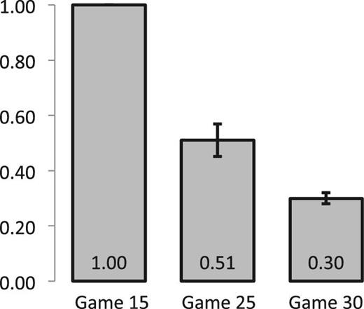
Efficiency levels in Experiment I, experienced games. The average efficiency levels and the corresponding 95% confidence intervals are reported for each game. Robust standard errors are obtained by clustering observations by session.

The statistical analysis of efficiency is documented in Tables 4 and 5. Table 4 reports the outcomes of a regression analysis in which we regress an indicator for whether the efficient match is reached (⁠|$\mathbb {1}_{\text{Eff}}$|⁠) on indicators for two out of three treatments (⁠|$\mathbb {1}_{\text{Game25}}$| and |$\mathbb {1}_{\text{Game30}}$|⁠), and these interacted with whether the first player in the game selected to be the proposer is a strong player or not (⁠|$\mathbb {1}_{\text{Strong First}}$|⁠):

$$\begin{eqnarray} \mathbb {1}_{\text{Eff}} &= \beta _0 + \beta _1 \cdot \mathbb {1}_{\text{Game25}} + \beta _2 \cdot \mathbb {1}_{\text{Game30}} + \beta _3 \cdot \mathbb {1}_{\text{Game15}} \cdot \mathbb {1}_{\text{Strong First}} \\ & \quad {} +\beta _4 \cdot \mathbb {1}_{\text{Game25}} \cdot \mathbb {1}_{\text{Strong First}} + \beta _5 \cdot \mathbb {1}_{\text{Game30}} \cdot \mathbb {1}_{\text{Strong First}} + \epsilon \, . \end{eqnarray}$$

Table 5 runs comparative tests of the coefficients from the regressions.

Table 4.

Efficiency in Experiment I, experienced games.

	Regression (1)	Regression (2)
Dependent variable	Efficiency	Efficiency
Constant (β0)	1.00*** (0.00)	1.00*** (0.00)
Game 25 (β1)	−0.49*** (0.03)	−0.34*** (0.03)
Game 30 (β2)	−0.70*** (0.01)	−0.47*** (0.04)
Strong first × Game 15 (β3)		0.00 (1.00)
Strong first × Game 25 (β4)		−0.37** (0.09)
Strong first × Game 30 (β5)		−0.49*** (0.04)
No. obs.	197	197
No. clusters	10	10
R-squared	0.2841	0.4238

Notes: Linear regressions with standard errors clustered at the session level are reported. **Significant at the 5% level; ***significant at the 1% level.

Table 5.

Hypothesis tests for efficiency in Experiment I, experienced games.

	Regression	Null hypothesis	Alternative hypothesis	p-value
Test 1	Regression (1)	β0 + β1 = β0 + β2	β0 + β1 > β0 + β2	p < 0.0001
Test 2	Regression (2)	β4 = β5	β4 > β5	p = 0.1042
Test 3	Regression (1)	β0 + β1 = 0.72	β0 + β1 < 0.72	p < 0.0001
Test 4	Regression (1)	β0 + β2 = 0.50	β0 + β2 < 0.50	p < 0.0001

Although all the final matches in Game 15, in the experienced games, are efficient, the probability that the efficient match is reached drops to 51% in Game 25 and even further to 30% in Game 30. Regression (1) and Test 1 confirm these changes. The positive and significant values of β₁ and β₂ in Regression (1) show that the decline in efficiency in Game 25 and Game 30 in comparison to Game 15 is significant (p < 0.0001 in both cases). Test 1 shows that there is also a significant decline in efficiency from Game 25 to Game 30 (p < 0.0001). With respect to the theoretical predictions outlined in Section 3.1, this monotonic decrease in efficiency is predicted by the MPE, but not by any other theory that we consider.

Furthermore, according to the MPE theory, whether or not the market clears efficiently in Games 25 and 30 depends on the network position of the first mover: If the first mover is a player with two links (strong player), then the market should end in an inefficient outcome with positive probability, whereas if it is a player with one link (weak player), then an efficient outcome will be reached with certainty.²⁸ The negative and significant values of β₄ and β₅ in Regression (2) support this prediction: Markets are less likely to reach efficient outcomes in Games 25 and 30, respectively, when the first player randomly selected to make a move is a strong player. The same is true if we condition the efficiency of the final match on the network position of the player who makes the first accepted offer. Details of this analysis are presented in Online Appendix D.1. Finally, Test 2 evaluates whether the decline in efficiency is larger in Game 30 compared with Game 25 when the first mover is the strong player, as also predicted by the MPE (p = 0.1084).

Despite the MPE making qualitative predictions about efficiency that are in agreement with our data, the quantitative predictions of MPE do not match the data so well. In Game 15, all the theories we considered predict that the efficient match will be reached for sure, and this is borne out in the data. Indeed, in every observation of Game 15 we have, the efficient match is reached. However, in Games 25 and 30, the MPE predicts that the rate of efficient matching will be 72% and 50%, respectively. Our observed rates of efficient matching are considerably lower. In Game 25, only 51% of markets reach an efficient outcome, which is significantly lower than the predicted 72% (p < 0.0001, Test 3). In Game 30, only 30% of markets reach an efficient outcome, which is also significantly lower than the predicted 50% (p < 0.0001, Test 4).

To summarize, we find strong evidence that matching is inefficient in Games 25 and 30, but not Game 15. This is only consistent with the MPE predictions of the theories we considered. Moreover, the various qualitative predictions made by the MPE about inefficient matching are borne out in the data. However, although the MPE does well qualitatively, there are significant deviations from its quantitative predictions. Interestingly, these deviations take the data further away from the predictions made by the other theories rather than towards them—there is even more inefficient matching than is predicted by the MPE.

5.2. Players’ Payoffs

Figure 3 presents the average payoffs of strong players (players A and D) and the average payoffs of weak players (players B and C) across our three treatments.

Figure 3.

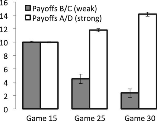
Players’ payoffs depending on their network position in Experiment I, experienced games. The average payoffs and the corresponding 95% confidence intervals are reported for each game. Robust standard errors are obtained by clustering observations by session.

The statistical analysis of players’ payoffs is documented in Tables 6 and 7. Table 6 reports regression analyses in which we regress players’ payoffs on indicators for different games (treatments); these indicators interacted with whether the player was strong (⁠|$\mathbb {1}_{\text{Strong}}$|⁠), and also interacted with whether the player exited the market first (⁠|$\mathbb {1}_{\text{Exit First}}$|⁠):

$$\begin{eqnarray} \text{Payoff} &= \beta _0 + \beta _1 \cdot \mathbb {1}_{\text{Game25}} + \beta _2 \cdot \mathbb {1}_{\text{Game30}} +\beta _3\cdot \mathbb {1}_{\text{Game15}} \cdot \mathbb {1}_{\text{Strong}} \\ & \quad {} +\beta _4 \cdot \mathbb {1}_{\text{Game25}} \cdot \mathbb {1}_{\text{Strong}}+ \beta _5 \cdot \mathbb {1}_{\text{Game30}} \cdot \mathbb {1}_{\text{Strong}} +\beta _6\cdot \mathbb {1}_{\text{Game15}} \cdot \mathbb {1}_{\text{Exit First}} \\ & \quad {} +\beta _7 \cdot \mathbb {1}_{\text{Game25}} \cdot \mathbb {1}_{\text{Exit First}}+ \beta _8 \cdot \mathbb {1}_{\text{Game30}} \cdot \mathbb {1}_{\text{Exit First}} + \epsilon . \end{eqnarray}$$

Table 6.

Players’ payoffs in Experiment I, experienced games.

	Regression (3)	Regression (4)
Dependent variable	Players’ payoffs	Players’ payoffs
	(all players)	(strong players in efficient matches)
Constant (β0)	10.04*** (0.03)	9.97*** (0.02)
Game 25 (β1)	−5.53*** (0.23)	0.13** (0.05)
Game 30 (β2)	−7.68*** (0.10)	−0.02 (0.04)
Strong × Game 15 (β3)	−0.07 (0.05)
Strong × Game 25 (β4)	7.26*** (0.25)
Strong × Game 30 (β5)	11.81*** (0.14)
Exit first × Game 15 (β6)		−0.01 (0.02)
Exit first × Game 25 (β7)		2.21*** (0.14)
Exit first × Game 30 (β8)		4.62*** (0.23)
No. obs.	788	218
No. clusters	10	10
R-squared	0.6977	0.8067

Notes: Linear regressions with robust standard errors clustered at the session level. Regression (3) considers payoffs of all players, whereas Regression (4) focuses on the payoffs of strong players (those with two links, players A and D) in the markets that reached an efficient outcome. **Significant at the 5% level; ***significant at the 1% level.

Table 7.

Hypothesis tests for players’ payoffs in Experiment I, experienced games.

	Regression	Null hypothesis	Alternative hypothesis	p-value
Test 5	Regression (3)	β0 + β1 = β0 + β2	β0 + β1 > β0 + β2	p < 0.0001
Test 6	Regression (3)	β0 + β1 + β4 = β0 + β2 + β5	β0 + β1 + β4 < β0 + β2 + β5	p < 0.0001
Test 7	Regression (4)	β7 = β8	β7 < β8	p < 0.0001

As the value of β₃ in Regression (3) is insignificant, there is no evidence that in Game 15 strong players receive higher payoffs. However, the significant values of β₄ and β₅ in Regression (3) show that strong players do receive higher payoffs in Game 25 and Game 30 than weak players. Furthermore, weak players receive statistically higher payoffs in Game 25 than in Game 30 (Test 5), whereas strong players obtain significantly lower payoffs in Games 25 than in Game 30 (Test 6).

Linking these observations regarding players’ payoffs back to the theories described in Section 3.1, we note that the observed trends are consistent with the predictions of all the theories. This is reassuring as it suggests that the theories we consider are able to capture key forces operating in our environment.

To further examine players’ payoffs across treatments, we consider whether the order in which players reach deals affects their payoffs, conditional on the final match being efficient.²⁹ In any perfect equilibrium of the dynamic game that reaches an efficient match, the pair of players exiting second receive the same payoff on average. This makes sense. These players end up in a bilateral bargaining game with a unique perfect equilibrium, and this equilibrium is symmetric. Thus, for all our noncooperative theories, the payoffs of strong players are predicted to be higher in Games 25 and 30 when they reach an agreement first, whereas the payoffs of weak players are predicted to be lower in Games 25 and 30 when they reach an agreement first.

These predictions are supported in the data. Figure 4 presents histograms of the final payoffs of the strong players by their order of exit and conditional on an efficient outcome being reached, where gray bars depict payoffs of players that exited the market first and black bars represent payoffs of players that exited the market second.³⁰ In Game 25, the average payoff of strong players is 12.3 if they exited first, whereas it is only 10.1 if they exited second. For weak players, it is 7.7 if they exited first and 9.9 if they exited second. Similarly, in Game 30, the average payoff of strong players is 14.5 if they exited first, whereas it is 10 if they exited second; the weak players’ average payoff is 5.5 when exiting first compared to 10 when exiting second. As reported in Table 6, the positive and significant coefficients on β₇ and β₈, but not on β₆, show that in Games 25 and 30, strong players do better when they move first, but there is no evidence that they do better moving first in Game 15. Furthermore, Test 7, reported in Table 7, shows that for the strong players, the relative benefit of moving first is larger in Game 30 than in Game 25 (p < 0.0001).

Figure 4.

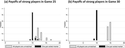
Distribution of strong player payoffs in efficient matches by the market composition at the time of exit, experienced games. In both figures, we consider only groups that reached an efficient match and focus on payoffs of strong players (players A and D).

We now turn to compare the quantitative outcomes observed in our experiments with the payoff predictions of the theories. These predictions and outcomes are summarized in Table 8 (along with, for ease of reference, predictions and outcomes for the rate of efficient matching).

Table 8.

Predicted versus observed outcomes in Experiment I, experienced games.

	Game 15			Game 25			Game 30
	eff.(%)	B (C)	A (D)	eff.(%)	B (C)	A (D)	eff.(%)	B (C)	A (D)
Theories
MPE all	100	10	10	72	6.45	11.45	50	4.17	13.33
MPE | eff.		10	10		8.95	11.05		8.34	11.67
Markov Reversion	100	10	10	100	8.75	11.25	–	–	–
Carrot and Stick	100	10	10	100	|$(7\frac{7}{9},9\frac{4}{9})$|	|$(10\frac{5}{9},12\frac{2}{9})$|	100	|$(6\frac{1}{9},9\frac{4}{9})$|	|$(10\frac{5}{9},13\frac{8}{9})$|
SPB	100	8.3	11.7	100	5	15	100	3.3	16.7
Core Midpoint	100	10	10	100	7.5	12.5	100	5	15
Core	100	[0, 20]	[0, 20]	100	[0, 15]	[5, 20]	100	[0, 10]	[10, 20]
Data
All	100	10	10	51	4.5	11.8	30	2.4	14.2
	(0.00)	(0.03)	(0.03)	(0.03)	(0.25)	(0.10)	(0.01)	(0.11)	(0.05)
| efficient		10	10		8.8	11.2		7.7	12.3
		(0.03)	(0.03)		(0.10)	(0.10)		(0.09)	(0.09)

Notes: The last four rows report efficiency rates and average payoffs of players by their network position, with the corresponding robust standard errors in the parentheses where observations are clustered at the session level. The first two rows under the category of Data report players’ payoffs and robust standard errors in all the final outcomes, whereas the last two rows under the category of Data focus on the groups that reached an efficient outcome.

In neither Game 25 nor Game 30 does any theory predict payoffs for both weak and strong players within a 95% confidence interval of those observed. Moreover, despite the EPE being able to support a range of payoffs (possibly even a larger range than the one we constructed if more complicated strategies were used), there does not exist an EPE that closely matches the observed payoffs in Game 30. As discussed in Section 3.1, in any EPE, the weak players must receive expected payoffs of at least 5, well outside the 95% confidence interval for the observed average payoffs of 2.4.

The average combined payoffs of players mechanically depend on the frequency with which an efficient match is reached. Given the high rate of inefficient matching observed in Game 25 and Game 30 treatments, considerably above the predicted rate of inefficient matching for any of the theories, it is impossible for any of the theories to do very well in their quantitative predictions of matching payoff. To strip away the efficiency dimension, and focus on the division of the surplus between strong and weak players, we also present the payoffs of players conditional on reaching an efficient outcome (last row of Table 8). For comparison, we also present the MPE-predicted payoffs of players who reach efficient outcomes (third row of Table 8). The MPE then predicts players’ payoffs within a 95% confidence interval in Game 25, and comes close to doing so in Game 30. There also then exist EPE strategies and core outcomes that generate consistent payoffs in both games.

5.3. Players’ Strategies

So far, market outcomes and market dynamics observed in our experiments fit well with the predictions of the MPE, and considerably better than with any of the other theories we have considered. In this section, we zoom in on the players’ strategies to determine whether MPE also provides helpful guidance for organizing the strategies used by our subjects. Although none of our subjects use strictly Markovian strategies,³¹ the analysis that follows shows that strategies used by our subjects are consistent with several qualitative features predicted by MPE.

The strategy of a player specifies a probability distribution over whom to make an offer to or choose the “Do Nothing” button, details of such offers (amounts kept), and the minimum amount a player is willing to accept from others after every possible history of play. The restriction to Markovian strategies only allows players’ strategies to depend on the state variable, which is the set of unmatched players. This greatly simplifies the strategy space and, given the structures of the markets we consider, there are just two different states for us to analyze. First is the state in which all the players are unmatched and active and the other is the one in which one of the efficient pairs has exited the market and the market consists of the one remaining strong player and one remaining weak player.

When only two players remain active in the market, both the weak and the strong players receive average payoffs of 10 in all three games, as the MPE predicts. Statistical analysis confirming this result is presented in Online Appendix D.2. Thus, in the remainder of this section, we focus on characteristics of strategies our experimental subjects use when all four players are unmatched and active.

We start by looking at the frequency with which players choose the “Do Nothing” button. As we have documented in the previous section, weak players earn more when they exit second rather than first. However, this should not incentivize weak players to delay in equilibrium because doing so increases the probability that they will be left unmatched. Nevertheless, do experimental subjects that are assigned weak positions in a network try to reach an agreement second? To answer this question, we look at the frequency with which players choose the “Do Nothing” button in each game. Pressing this button can be seen as the manifestation of delay, that is, the choice not to make a proposal. Our data show that players almost never choose to delay, irrespective of their network position: There are no delays in Game 15, one instance of a delay in Game 25 (0.64%) by a strong player, and three instances of delays in Game 30 (1.56%), two of which are by a weak player and one by a strong player. Statistical analysis confirms that there is no significant difference between the frequency of delays between the strong and weak players in both Game 25 and Game 30 (see Online Appendix D.2). The absence of delay also provides some support for subjects using simple strategies.

Next, we examine the frequency with which strong players make offers to their efficient partners rather than to each other when all players are present in the market. The MPE predicts that this frequency is 100% in Game 15, 42% in Game 25, and 0% in Game 30. In Figure 5, we present the empirical histogram of strong players’ individual frequencies of proposing efficiently in each game. Because the MPE predicts that an agreement will always be reached in the first round, we restrict our attention to first-round proposals. The observed proposal frequencies, across the three treatments, fit the MPE theory well. As Figure 5 shows, we observe a significant shift in the strategies used by the strong players as the value of the diagonal link increases. In particular, in Game 15 over 80% of subjects always propose only to their efficient partner in every game in which they are assigned to a strong bargaining position. In contrast, in Game 30, over 80% of subjects never propose to their efficient partner when in strong bargaining positions. To confirm this, we regress an indicator for a strong player making a proposal to their efficient partner (⁠|$\mathbb {1}_{\text{Strong Proposes Efficient Match}}$|⁠) on indicators for the treatments (games):

$$\begin{eqnarray} \mathbb {1}_{\text{Strong Proposes Efficient Match}} &= \beta _0 + \beta _1 \cdot \mathbb {1}_{\text{Game25}} + \beta _2 \cdot \mathbb {1}_{\text{Game30}} + \epsilon . \end{eqnarray}$$

Figure 5.

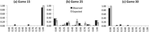
Frequency of efficient proposals by strong players, experienced games. For each subject, we compute the frequency of proposing to her efficient partner in the first round of the last five repetitions conditional on this player being assigned a strong position. Black bars are the observed frequencies. Light gray bars take the distribution over the number of offers different players make from the data, and then simulate the frequencies with which these players make efficient offers assuming that they all play exactly the strategy prescribed by MPE. We run 10,000 simulations and report the average frequencies as well as the range of frequencies between the 5th and 95th percentiles.

The regression analysis, reported in Table 9, confirms that subjects in strong network positions are more likely to make efficient proposals in Game 15 than in Game 25 and Game 30.³²

Table 9.

Regression analysis of frequency of efficient proposals by strong players in Experiment I, experienced games.

	Regression (5)
Dependent variable	Indicator of proposing efficiently by a strong player
	(four players are active)
Constant (β0)	0.95*** (0.03)
Game 25 (β1)	−0.56*** (0.04)
Game 30 (β2)	−0.85*** (0.04)
No. obs.	428
No. clusters	10
R-squared	0.2518

Notes: Linear regression with robust standard errors clustered at the session level. ***Significant at the 1% level.

Next, we consider the amount that players propose to keep for themselves when making an offer and compare this to the amounts predicted by the MPE. Table 10 reports these average ask amounts by offer type, distinguishing between offers from strong players to strong players, weak players to strong players, and strong players to weak players.³³ On average, observed ask amounts are close to those predicted by MPE. The closest fit we get are for the offers from strong to weak players for which the MPE predicted offers fall into the 95% confidence intervals of those observed in our experimental data. In terms of deviations from the MPE, the strong players tend to ask for less than predicted when making offers to each other, whereas the weak players ask for more than predicted when making offers to the strong players in Game 30. All else equal, this helps the strong players to reach an agreement with each other and hinders the weak players from reaching an agreement with the strong players.

Table 10.

Predicted and observed ask amounts when all players are unmatched in Experiment I, experienced games.

	Game 15		Game 25		Game 30
	MPE	DATA	MPE	DATA	MPE	DATA
		mean (robust st err)		mean (robust st err)		mean (robust st err)
		[95% CI]		[95% CI]		[95% CI]
Strong to strong	–	–	13.55	12.79 (0.10)	16.67	15.27 (0.04)
				[12.49, 13.10]		[15.12, 15.42]
Strong to weak	10	10.54 (0.13)	13.55	13.27 (0.42)	–	–
		[9.96, 11.12]		[11.92, 14.21]
Weak to strong	10	10.62 (0.14)	8.55	9.07 (0.37)	6.67	7.86 (0.17)
		[10.02, 11.22]		[7.89, 10.26]		[7.13, 8.60]

Notes: For the observed ask amounts, we report average ask amounts when the markets are complete (all four players are active). Robust standard errors are reported in the parentheses, where observations are clustered by session. CI–confidence interval. A “–” indicates that the MPE predicts no offers of this kind.

The low offers made by weak players to strong players would result in surplus being more equitably distributed between the strong and weak players if accepted. Indeed, we frequently observe weak players demanding exactly equitable splits of 10 each in both Game 25 and Game 30. In Game 25, for the experienced games when all players are active, 50% of weak subjects ask for an even split sometimes. In Game 30, the corresponding percentage is 68%. Of the 50% in Game 25 who sometimes propose equal splits, the average frequency with which an equal split is demanded is 60%. In Game 30, it is 50%.³⁴

A similar picture emerges from the analysis of offers that subjects accept and those they reject as responders.³⁵ Consistent with MPE predictions, as the value of the diagonal link increases, strong responders tend to accept higher offers, whereas weak responders settle for lower shares. However, although the aforementioned qualitative difference between treatments is in line with the MPE, there are also some notable deviations. Strong players’ acceptance strategies are roughly in line with the MPE predictions. In Game 25, they accept 84% of offers above their predicted continuation value of rejecting, 11.45 (69 out of 82 cases), and reject 86% of offers below 11.45. In Game 30, they accept 89% of offers above their predicted continuation value of rejecting, 13.33, and reject 93% of offers below 13.33. At the same time, weak players’ acceptance strategies are often at odds with the MPE. Theoretically, weak players should accept payoffs weakly above 6.45 in Game 25. In practice, they reject 50% of proposals from the strong players that offered them strictly less than an equal split of 10, but more than 6.45.³⁶ In Game 30, weak players should never receive an offer, and in line with this there are too few observations of weak players receiving offers for us to evaluate their acceptance strategies. These deviations again make it less likely that strong and weak players will reach an agreement with one another.

5.4. Horse Race Between Theories

Overall we interpret the evidence from Experiment I as providing broad support for the MPE theory over the other theories, and consider that the MPE organizes the data well. The data match the MPE theory on many, albeit related, dimensions qualitatively, but differ from the quantitative predictions.

Table 11 summarizes the qualitative performance of the different theories. The theories generally do well at describing how the payoffs of the strong and weak players vary across games, and the noncooperative theories also predict how this depends on whether they exit first or second. However, these theories perform differently in terms of their efficiency predictions. Whereas the EPE theories and cooperative theories predict no inefficiencies, the MPE predicts, as we observe, that there will be no inefficiencies in Game 15, but that inefficiencies then increase monotonically moving from Game 15 to Game 25, and then to Game 30. Also, in terms of strategies, the MPE does a little better. All the theories correctly predict that players do not delay by making no offer, but the MPE is the only theory that predicts that strong players offer to each other with increasing frequency as we move from Game 15 to Game 25 to Game 30. Indeed, the MPE theory also does relatively well quantitatively in this dimension.

Table 11.

Predicted versus observed outcomes in the experienced games.

	Cooperative theories			Noncooperative theories
			Core		Markov	Carrot
	Core	SPB	midpoint	MPE	reversion	and Stick
Efficiency
(1) Matching is efficient in Game 15	✓	✓	✓	✓	✓	✓
(2) The rate of efficient matching declines from Game 15 to Game 25 to Game 30	✗	✗	✗	✓	✗	✗
(3) Games 25 and 30: Efficient outcomes are more likely to be reached if a weak player proposes first	✗	✗	✗	✓	✗	✗
Players’ payoffs
(1) Strong players’ payoffs increase from Game 15 to Game 25 to Game 30	–	✓	✓	✓	✓	✓
(2) Weak players’ payoffs decrease from Game 15 to Game 25 to Game 30	–	✓	✓	✓	✓	✓
(3) Difference in payoffs of strong players in efficient matches from exiting first rather than second is positive and higher in Game 30 than in Game 25	–	✗	✗	✓	✓	–
Players’ strategies
(1) Players do not delay	–	–	–	✓	✓	✓
(2) Frequency of efficient proposals by strong player declines from Game 15 to Game 25 to Game 30	–	–	–	✓	✗	✗

Notes: When a theory is consistent with the data and would be violated by the opposite finding, we mark the cell with a ✓. If the theory does not make this prediction, but is consistent with it, we mark the cell with a –, and if the predictions of the theory are violated by the data, we mark the cell with a ✗.

Our paper thus joins the emerging experimental literature that examines MPE in a variety of dynamic games (see Battaglini and Palfrey 2012; Battaglini, Nunnari, and Palfrey 2016; Salz and Vespa 2020; Vespa 2016). Similar to our results, in combination, these papers show that comparative statics predictions implied by MPE organize experimental data quite well across a variety of dynamic games. Simplicity seems to provide useful guidance for equilibrium selection, even when, as in our case, it runs contrary to efficiency.

5.5. An Adjustment to the MPE

Whereas we view the MPE as doing a good job of capturing some of the key forces at play, the systematic deviations from the quantitative predictions suggest that it is also missing something. To gain a better understanding of what this might be, it is helpful to consider again the systematic deviations from players’ MPE strategies that we observe in the data.

We have seen that weak players are frequently unwilling to reach inequitable agreements they should be willing to reach according to the MPE. This is reflected both in them offering less to strong players than they should and in them refusing to accept offers they should. Taking inspiration from the large experimental literature analyzing two-person bargaining games (see Roth 1995 for a survey), and motivated by our analysis of players’ strategies, suppose that some players always demand an equal share of surplus with their efficient partner, whereas others, whom we term rational, seek to maximize their expected payoffs.

As already noted, because weak players often demand a higher share of surplus than predicted by the MPE, they often fail to reach agreements when proposing or receiving an offer. The same does not apply when strong players are making offers to each other. Indeed, the likelihood of reaching an agreement in the first round is significantly higher if the first mover is a strong player rather than a weak player.³⁷ This can account for inefficient agreements being reached with a higher frequency than predicted by the MPE. Furthermore, as weak players get a payoff of zero in these cases, the payoffs of strong and weak players are also likely to be less equal than predicted. So, the presence of weak players demanding too much can help explain both the observed deviations in the rate of efficient matching from the MPE predictions, and the deviations in the average payoffs of weak and strong players.³⁸

In Online Appendix Section F, we develop this idea in more detail by calculating the MPE of an extended model that includes some behavioral players. The behavioral players always demand a payoff of at least 10 when both proposing and accepting. We find that by adjusting the MPE in this way it can do a considerably better job of matching the data quantitatively.

Interestingly, and in contrast to the ultimatum game where evidence for the presence of behavioral players like this has also been documented, the introduction of behavioral types demanding equality results in more unequal outcomes as well as more inefficient outcomes being predicted. Strong players respond to the demands of these behavioral weak players by more frequently excluding them from agreements, yielding more mismatch and inequality. Rules of thumb that are adopted by some players and do well in limiting inequality in the ultimatum game also seem to be adopted in our setting, but with the consequence of exacerbating inequality.³⁹

5.6. Key Forces and External Validity

There are two key things that we take away from Experiment I. First, even in our simple setting, markets very frequently fail to reach efficient outcomes. Second, bargaining positions matter. Strong players, those with two links, do better than weak players, those with one link, and how much better depends on the value of their alternative match. Players’ payoffs also depend on the market composition at the time they exit. Strong players do better if they reach an agreement when both matches are still available to them.

This raises crucial questions about the possibility of the bargaining frictions we find in the laboratory also being present in practice. In real-world high-skill markets, with limited search and informational frictions, will there still be a serious impediment to the efficient matches being reached in the form of bargaining frictions? If bargaining frictions do matter in such markets, might they also exacerbate problems in other markets more prone to search and informational frictions?

Addressing these questions is hard. The laboratory setting is removed from the real world in several ways. Nevertheless, better understanding what is driving the inefficiency we find in the laboratory can help to inform us better about the likelihood of bargaining frictions having a substantial impact in real markets. To this end, we advance two related explanations about what might be underlying the inefficiencies we find.

We know that whenever an inefficient match occurs, there are at least two players who have a deviation to match with each other that can make them both strictly better off. So, in our experiment, there are pairs of participants who are leaving surplus on the table. Moreover, there are simple heuristics that exploit profitable deviations and if followed, will lead the market to converge to a pairwise stable and efficient outcome (see, for example, Bayati et al. 2015). Two related features of our experimental design could be causing problems that prevent this logic from being realized. First, the presence of a rigid protocol governing who can interact with whom and when might be preventing participants (in weak bargaining positions) who are about to be excluded from making offers that would exploit a profitable pairwise deviation. For example, after a weak player’s efficient partner has received an offer to match inefficiently, this offer must be accepted or rejected before the weak player has the chance to put a counterproposal on the table. Second, agreements are reached sequentially, and after a proposal has been accepted, the players in question exit the market, preventing them from exploiting profitable pairwise deviations that might remain. If, instead, players could renege on agreements, there would be no impediment to profitable pairwise deviations being exploited and efficient outcomes might be reached.⁴⁰

Although our two explanations are closely related to each other, they have different implications for the conclusions that can be drawn from our experiment. If it is the experimental protocol that is generating the inefficiencies we find, then the external validity of our experiment would be quite limited. In the real world, interactions are not constrained by a protocol. If, instead, it is the sequential order in which agreements are reached, and the inability of people to renege on deals, external validity is less compromised. Jobs in labor markets are typically filled sequentially, whereas firms very rarely renege on agreements and it is unusual for people to do so too.⁴¹

To test these explanations and better understand what is driving inefficiencies in Experiment I, we run two new experiments. In Experiment II, we allow the participants to interact freely with each other and do not impose an experimental protocol on interactions. In Experiment III, we allow people to renege on existing agreements, for a small cost; otherwise, the protocol from the first experiment is maintained.

6. Experiment II: Unstructured Bargaining

6.1. Experimental Design and Procedures

Experiment II consists of one treatment, which uses the market structure of Game 30 (see Figure 1). This treatment was conducted at the University of California, Irvine. A total of 88 subjects participated in three experimental sessions, which lasted less than 1 hour, including the instruction period and quiz. Subjects earned on average $23.5, including a $15 showup fee.

Similarly to the Game 30 treatment of Experiment I, in each session of Experiment II, subjects play ten repetitions of Game 30 with random rematching between games. Within each game there is no predetermined structure of bargaining. Instead, subjects can make offers to any other player they might match with, withdraw offers they have previously proposed, and accept any currently standing offer they have received. Just like in Experiment I, offers specify the player to whom it is made as well as the surplus split.⁴² Once an offer is accepted, the match between these two players is formed and these players exit the market, that is, have no more opportunities to move in the game. When a match is formed, all currently standing offers are voided, and bargaining starts afresh. Similarly to Experiment I, there are two ways in which the game can come to an end in Experiment II. First, the game ends if there are no new matches that can be formed between any two subjects who are not matched yet. Second, the game may end because of discounting, implemented as a random termination of the game: There is a 1% chance that the game ends at the end of each 30-second interval. When the game ends, unmatched players receive a payoff of 0, whereas matched players earn payoffs according to their agreements. We refer the reader to Online Appendix Section J for the complete instructions used in these sessions as well as the screenshots and the quiz that subjects were asked to complete before the beginning of the experiment.

6.2. Results

Our approach to the data analysis is the same as in Experiment I. In particular, we focus on behavior in the experienced games (the last five repetitions of the game in each session) and perform most of the tests using a regression analysis with standard errors clustered by session.

Our data show that with unstructured bargaining markets continue to often match players inefficiently. In Experiment II, Game 30, the market cleared efficiently only 59% of the time. This is better than in Experiment I, Game 30, which had an efficiency rate of 30%, but considerably less than all the time.

To investigate this further, we run the following regression on our Game 30 data from Experiments I and II, |$\mathbb {1}_{\text{Eff}} = \beta _0 + \beta _1 \cdot \mathbb {1}_{\text{Exp II}} + \epsilon$|⁠. This confirms that the efficiency rate in Experiment II, Game 30 is higher than that in Experiment I, Game 30 [p < 0.0067, Regression (6) reported in Table 12].

Table 12.

Efficiency and players’ payoffs in Experiment I versus Experiment II for Game 30, experienced games.

	Regression (6)	Regression (7)	Regression (8)
Dependent variable	Efficiency	Players’ payoffs	Players’ payoffs
		(strong players)	(weak players)
Constant	0.30*** (0.01)	14.17*** (0.05)	2.36*** (0.10)
Experiment II	0.29*** (0.06)	−0.89*** (0.26)	5.53*** (0.35)
No. obs.	179	357	269
No. clusters	6	6	6
R-squared	0.0779	0.0296	0.3856

Notes: Linear regression with robust standard errors clustered at the session level. Regression (7) concerns payoffs of strong players only, whereas Regression (8) focuses on payoffs of weak players only. ***Significant at the 1% level.

To compare players’ payoffs by their bargaining positions across Experiments I and II, we run the regression, |$\mathbb {1}_{\text{Payoff}} = \beta _0 + \beta _1 \cdot \mathbb {1}_{\text{Exp II}} + \epsilon$|⁠, for strong and then weak players. Weak players earn significantly and substantially higher amounts in Experiment II than in Experiment I [see Regression (8) in Table 12]. The difference between payoffs of strong players in Experiments I and II is significant but negative and rather small. Weak players appropriate all the additional gains from trade obtained from the higher rates of efficient matching in Experiment II, and then a little bit more.

Figure 6 shows the histogram of the final payoffs of the strong players in the Experiment II, Game 30 treatment by their order of exit, and conditional on an efficient outcome being reached. The gray bars in this figure depict the payoffs of players that exited the market first and black bars present the payoffs of players that exited the market second.

Figure 6.

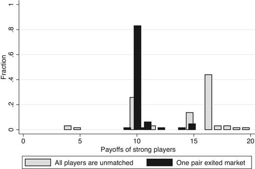
Payoffs of strong payers in efficient matches in Game 30 in Experiment II by market composition at the time of exit, experienced games. We consider only groups that reached an efficient match.

The average payoff of strong players is 13.8 if they exited first, and it is 10.4 if they exited second, whereas the weak players earn on average 6.2 when exiting first compared to 9.6 when exiting second. This suggests that strong players continue to benefit from reaching an agreement first in Experiment II.

To confirm these observations, we regress players’ payoffs on an indicator for whether they are strong or not, and whether they exited the market first:

$$\begin{eqnarray} \text{Payoff} &=& \beta _0 + \beta _1 \cdot \mathbb {1}_{\text{Strong}} + \beta _2 \cdot \mathbb {1}_{\text{Exit First}}+ \epsilon . \end{eqnarray}$$

Similarly to the Experiment I, Game 30 treatment, we observe that the strong players obtain higher payoffs than the weak players [see Regression (9) in Table 13]. Moreover, as in the Experiment I, Game 30 treatment, in the Experiment II, Game 30 treatment, the order of exit also continues to matter. Regression (10) in Table 13 confirms that strong players benefit from exploiting their bargaining position when they exit the market first rather than second.

Table 13.

Players’ payoffs in Game 30 in Experiment II, experienced games.

	Regression (9)	Regression (10)
Dependent variable	Players’ payoffs	Players’ payoffs
	(all players)	(strong players in efficient matches)
Constant (β0)	4.70*** (0.57)	10.38*** (0.11)
Strong (β1)	8.52*** (0.77)
Exit first (β2)		3.38** (0.69)
No. obs.	440	130
No. clusters	3	3
R-squared	0.5510	0.2953

Notes: Linear regressions with robust standard errors clustered at the session level. Regression (9) concerns payoffs of all players, whereas Regression (10) focuses on the payoffs of strong players (players A and D) in the markets that reached an efficient outcome. **Significant at the 5% level; ***significant at the 1% level.

To sum up, when our experimental subjects can act as they see fit in an unstructured manner, substantial inefficiencies persist and our data show strong support for the market composition continuing to affect the payoffs of the players.

Experiment II Conclusions.

There are two main things we take away from Experiment II. First and foremost, despite allowing for unstructured bargaining, we continue to find high rates of mismatch, albeit lower than in Experiment I. Second, bargaining positions continue to matter. Players with two links do better than players with one link when both links are still available, but not once their alternative match has left the market.

There is a simple logic we expound in the Introduction that can explain why it is hard to get efficient matching. Suppose there are two parties who match with each other in the efficient match, but that one of them is in a stronger bargaining position than the other. If the efficient match is reached for certain, then the player in the weaker bargaining position can wait for others in the market to exit until she is no longer in a weak position. But given this, strong players would strictly prefer to match inefficiently, and in contradiction to the premise, we would not reach the efficient match for sure. This logic is reflected in the results from Experiment II, as well as those from Experiment I. In both experiments, players whose bargaining position might deteriorate sometimes match inefficiently. This creates a real prospect that weak players will find themselves unmatched, and it is likely that this plays a role in persuading weak players to accept lower payoffs (thus allowing the strong players to gain from their bargaining positions).

7. Experiment III: Reneging Experiment

We now test the hypothesis that if we limit the nonstationarities in bargaining positions, efficient outcomes will be obtained. We test this hypothesis by running Experiment III, in which we allow players to renege on existing agreements for a small cost.

7.1. Design and Procedures

The design and experimental procedures of Experiment III are very similar to those of the Experiment I. Experiment III consisted of three treatments, Game 15, Game 25, and Game 30, with each treatment corresponding to one of the markets described in Figure 1.⁴³ Just like Experiment I, Experiment III was conducted in the same two locations: at the ESSL at the University of California, Irvine and at the EBEL at the University of California, Santa Barbara. A total of 10 sessions were run, with a total of 156 subjects, recruited from a database of undergraduate students enrolled in these universities.⁴⁴ The experiments lasted about 2 hours. Average earnings, including a $15 showup fee, were $23.7 with a standard deviation of $4.9.

In each session, subjects played ten repetitions of the same game, with random rematching between games. The main feature of Experiment III is the possibility of reneging on agreements formed in previous rounds. Recall that in Experiment I players have no opportunity of reneging, as those who reach agreements are forced to exit the market permanently, which means they cannot make any further moves.⁴⁵ On the contrary, in Experiment III, players who reach agreements do not exit the market and can unilaterally break agreements they are part of at a small cost c.⁴⁶ In all three treatments of Experiment III, we used the same separation cost of c = 10 cents per broken agreement. Thus, a player who has formed a match remains active and can both propose new matches and accept new offers when proposed to her. If a currently matched player accepts a new offer, then she pays the separation cost for dissolving the previous match she was involved in and forms a new match in its place. If a currently matched player makes a new offer, which is accepted by the responder, then the proposer pays the separation cost for breaking the match she was part of. The person who was part of an agreement that is broken by their partner in the current round does not pay the separation cost, but starts the next round unmatched. At the top of the screen, subjects were reminded of the separation cost and of the number of times they have paid it in the current game.

All the remaining protocol details of Experiment III mirror those of Experiment I. In particular, there are two ways in which a game can end. First, there is a 1% chance that the game ends after each round, determined by a random draw of the computer. Second, the game ends if there was no positive surplus remaining between any pair of players who both made proposals in the last round.

7.2. Results

In this section, we report several key comparisons of final outcomes observed in Experiments I and III. As before, we focus on the experienced games and use regressions with standard errors clustered at the session level to perform statistical analysis.

The premise of Experiment III is that the ability of players to renege on their current deals will make the bargaining environment stationary. To investigate the validity of this premise, we compare the monetary offers that unmatched strong players receive and accept, and the offers unmatched strong players make and have accepted, when (i) all players are unmatched versus (ii) when the other strong player has already formed a tentative match with their efficient partner.

Table 14 shows that there is little evidence, in any of the three treatments, Game 15, Game 25, or Game 30, that the offers received or made by unmatched strong players, conditional on being accepted or not, depend on whether the other strong player was matched or not. This corroborates our hypothesis that, if reneging is possible, the bargaining positions of players remain relatively stationary, irrespective of whether the other players in the market are matched or not.

Table 14.

Offers made to and received by unmatched strong players in Experiment III, experienced games.

	Game 15			Game 25			Game 30
	No match	Match	p-value	No match	Match	p-value	No match	Match	p-value
Offer made	10.57	10.43	0.52	12.98	12.30	0.09	15.54	15.41	0.71
And accepted	9.21	9.70	0.18	9.41	9.32	0.93	10.56	9.38	0.27
Offer received	9.71	9.31	0.30	11.77	11.67	0.79	13.58	13.14	0.46
And accepted	10.00	10.00	1.00	12.30	12.06	0.59	14.56	14.48	0.21

Notes: This table reports the efficient offers made by strong players (i.e. those to their efficient match), the accepted efficient offers made by strong players, the efficient offers received by strong players, and the accepted efficient offers received by strong players. It does so for (i) when all players are unmatched (no match); and (ii) when the other strong player is efficiently matched (match). The offers made by the strong players correspond to the amount the strong players proposed to keep for themselves. The offers received by strong players correspond to the payoffs the strong players get if these offers are accepted by them. The p-values are computed based on the regressions, in which we regress the observed offers on a constant and an indicator for one of the groups, while clustering standard errors by session.

Our main hypothesis is in regard to a comparison of the efficiency levels observed in Experiment I with those observed in Experiment III. Figure 7 depicts the efficiency in each treatment in the experienced games, along with the 95% confidence intervals. As expected, in Game 15 we observe almost full efficiency, regardless of the possibility of renegotiation. In the remaining two games, the possibility of reneging affects the final outcomes and significantly increases efficiency: In Game 25, efficiency increases from 51% to 82%, and in Game 30, it increases from 30% to 73%.

Figure 7.

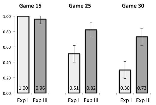
Efficiency of the final match in Experiments I and III, experienced games. Average efficiency per treatment is reported, along with the 95% confidence interval, computed using robust standard errors, where errors are clustered at the session level.

To confirm that these differences are statistically significant, we combine our data from Experiments I and III and regress an indicator for whether the efficient match is reached on indicators for the treatments within the experiments (Game 15, Game 25, Game 30), and these treatment indicators interacted with an indicator for Experiment III (⁠|$\mathbb {1}_{\text{Experiment III}}$|⁠):

$$\begin{eqnarray} \mathbb {1}_{\text{Eff}} &= \beta _0 + \beta _1 \cdot \mathbb {1}_{\text{Game25}} + \beta _2 \cdot \mathbb {1}_{\text{Game30}} + \beta _3 \cdot \mathbb {1}_{\text{Game15}} \cdot \mathbb {1}_{\text{Experiment III}} \\ & \quad {}+\beta _4 \cdot \mathbb {1}_{\text{Game25}} \cdot \mathbb {1}_{\text{Experiment III}} + \beta _5 \cdot \mathbb {1}_{\text{Game30}} \cdot \mathbb {1}_{\text{Experiment III}} + \epsilon . \end{eqnarray}$$

Regression analysis confirms that in Games 25 and 30 efficiency levels achieved in Experiment III are significantly higher than those achieved in Experiment I: Estimated coefficients β₄ and β₅ are positive and significant in Regression (11) presented in Table 15 (p < 0.01 for the coefficients).⁴⁷

Table 15.

Efficiency in Experiments I and III, experienced games.

	Regression (11)	Regression (12)
Dependent variable	Efficiency	Efficiency
	Games 15, 25, and 30	Games 25 and 30
	Experiments I and III	Experiment III only
Constant (β0)	1.00*** (0.00)	0.73*** (0.02)
Game 25 (β1)	−0.49*** (0.03)	0.09 (0.04)
Game 30 (β2)	−0.70*** (0.01)
Experiment III × Game 15 (β3)	−0.04** (0.02)
Experiment III × Game 25 (β4)	0.32*** (0.05)
Experiment III × Game 30 (β5)	0.42*** (0.02)
No. obs.	369	127
No. clusters	20	7
R-squared	0.2735	0.0130

Notes: Linear regression with robust standard errors clustered at the session level. **Significant at the 5% level; ***significant at the 1% level.

Although there is no statistical difference between the efficiency levels observed in the Game 25 and Game 30 treatments in Experiment III (see Regression (12) reported in Table 15), these levels are statistically less than 100% and so some inefficiency remains.⁴⁸

We report the payoffs of players in Experiment I and Experiment III in Table 16. To confirm the patterns apparent in Table 16, we regress their payoffs on indicators for the different games, and these interacted with an indicator for Experiment III:

$$\begin{eqnarray} \text{Payoffs} &= \beta _0 + \beta _1 \cdot \mathbb {1}_{\text{Game25}} + \beta _2 \cdot \mathbb {1}_{\text{Game30}} + \beta _3 \cdot \mathbb {1}_{\text{Game15}} \cdot \mathbb {1}_{\text{Experiment III}} \\ & \quad {}+\beta _4 \cdot \mathbb {1}_{\text{Game25}} \cdot \mathbb {1}_{\text{Experiment III}} + \beta _5 \cdot \mathbb {1}_{\text{Game30}} \cdot \mathbb {1}_{\text{Experiment III}} + \epsilon \, . \end{eqnarray}$$

Table 16.

Payoffs of players by network position in Experiments I and III, experienced games.

	Game 15		Game 25		Game 30
	B (C)	A (D)	B (C)	A (D)	B (C)	A (D)
All final matches
Experiment I	10.0 (0.03)	10.0 (0.03)	4.5 (0.25)	11.8 (0.10)	2.4 (0.11)	14.2 (0.05)
Experiment III	9.8 (0.12)	9.8 (0.09)	6.2 (0.35)	12.3 (0.16)	3.6 (0.05)	14.8 (0.15)
Efficient final matches
Experiment I	10.0 (0.03)	10.0 (0.03)	8.8 (0.10)	11.2 (0.10)	7.7 (0.09)	12.3 (0.09)
Experiment III	10.0 (0.03)	10.0 (0.03)	7.5 (0.18)	12.3 (0.08)	4.9 (0.18)	15.0 (0.14)

Notes: We report average payoffs of players by their network positions, with the corresponding robust standard errors in the parentheses, where observations are clustered at the session level.

Table 17.

Players’ payoffs in Experiments I and III, experienced games.

	Regression (13)	Regression (14)	Regression (15)	Regression (16)
Dependent variable	Payoffs	Payoffs	Payoffs	Payoffs
	Strong players	Weak players	Strong players	Weak players
			efficiently matched	efficiently matched
Constant (β0)	9.97*** (0.03)	10.03*** (0.03)	9.96*** (0.03)	10.03*** (0.03)
Game 25 (β1)	1.80*** (0.09)	−5.53*** (0.22)	1.24*** (0.08)	−1.24*** (0.09)
Game 30 (β2)	4.20*** (0.05)	−7.68*** (0.09)	2.30*** (0.05)	−2.30*** (0.08)
Experiment III × Game 15 (β3)	−0.18** (0.08)	−0.27** (0.10)	0.05 (0.04)	−0.05 (0.04)
Experiment III × Game 25 (β4)	0.52*** (0.17)	1.71*** (0.38)	1.15*** (0.12)	−1.31*** (0.18)
Experiment III × Game 30 (β5)	0.67*** (0.14)	1.26*** (0.10)	2.69*** (0.14)	−2.85*** (0.17)
No. obs.	740	740	502	502
No. clusters	20	20	20	20
R-squared	0.5726	0.4243	0.6860	0.6543

Notes: Linear regression with robust standard errors clustered at the session level. **Significant at the 5% level; ***significant at the 1% level.

The positive and significant values of β₄ and β₅ in Regressions (13) and (14) (p < 0.01) show that in Games 25 and 30 both strong and weak players receive higher payoffs in Experiment III than in Experiment I. However, the average payoffs of the players have to be higher because of the higher rate of efficient matching, so these regressions just tell us that these gains are shared among the strong and weak players (although the weak players seem to benefit a little more). However, conditional on an efficient match being reached, strong players’ payoffs increase, whereas weak players’ payoffs decrease (Regressions (15) and (16)). This makes sense. The advantageous bargaining positions of strong players are transitory in Experiment I, but more permanent in Experiment III.

Takeaways from Experiment III.

There are two main things we take away from Experiment III. First, bargaining positions continue to matter, but unlike before there is no evidence that they change as agreements are reached. Our intention was to make the environment more stationary, and, reassuringly, the evidence is consistent with this. Second, and more important, with more stationary bargaining positions efficiency increases quite considerably, although nontrivial and statistically significant rates of mismatch remain.

8. Conclusions

Market clearing is a fundamental question in economics. It is important to get the “right” people into the “right” jobs, especially in the high-skill labor markets in which mismatches can be very costly in terms of efficiency. In this paper, we remove standard frictions and study mismatch. We turn off search frictions by letting players be patient, remove information problems by giving everyone symmetric information about match surpluses, remove coordination problems by considering very simple markets, and give norms a good chance of yielding the efficient outcome by considering markets in which a perfectly equitable and efficient outcome is feasible. We still find persistent and extensive mismatches across our three experiments.

Inefficiencies are highest when interactions are constrained by an experimental protocol and participants are not permitted to renege on agreements they reach. In this experiment (our main experiment), the MPE of the corresponding bargaining game does a good job of organizing the data across a variety of dimensions. This includes market outcomes as well as a more nuanced prediction regarding players’ strategies. Nevertheless, some participants’ strategies are suggestive of systematic deviations that exhibit a particular behavioral bias—similarly to previous experimental work on the ultimatum game, some players in weak positions demand a more equitable split of surplus than theory suggests they should. However, unlike in the ultimatum game, in our setting this reduces efficiency and makes outcomes less equal. Instead of being offered more, behavioral players are left unmatched more often, and market outcomes are both less efficient and less equitable than predicted by the MPE.

We remove the bargaining protocol in Experiment II, thereby permitting much richer endogenous interactions, and inefficiency improves but remains substantial. This suggests that the results from the first experiment are not just driven by the rigid bargaining protocol. Permitting agents to renege on agreements, which makes the environment more stationary, efficiency improves more, but again nontrivial inefficiencies persist. As bargaining positions seem nonstationary in many high-skill labor markets, we view our results as being consistent with the bargaining frictions we document contributing towards mismatch in actual markets. Frictions in our experiment arise because of both the protocol and the commitment. Although we view the constraints put on interactions by the protocol as an unrealistic representation of interactions in real markets, there is often a commitment.

Acknowledgements

We thank Federico Echenique, Edoardo Gallo, Ben Gillen, Ben Golub, Jörg Kalbfuss, Francesco Nava, Emanuel Vespa, Leeat Yariv, and participants in seminars at Berkeley HAAS, Berlin, Bonn, Cologne, Columbia, EUI, Georgetown, NYU, Pittsburgh, Queen Mary, Tel Aviv, UCL, and UCSD for helpful comments and suggestions. Financial support from the European Research Council under the grant EMBED #757229 (Elliott) is gratefully acknowledged.

Notes

The editor in charge of this paper was Juuso Välimäki.

Appendix A: Experiment I: Markov Perfect Equilibria

In this section, we derive the MPE predictions summarized in Section 3.1. A more formal and general derivation is provided in Elliott and Nava (2019). We start with Game 25. Let W(δ) be the continuation value of players in the subgames where they are bargaining bilaterally with their efficient partners. By Rubinstein (1982) there is a unique perfect equilibrium in these subgames and lim_δ→1W(δ) = 10. Letting V_i be the continuation value of player i when no one has yet been matched, we look for a symmetric solution in which V_A = V_D ≔ V_S is the continuation value for both the strong players and V_B = V_C ≔ V_W is the continuation value for both the weak players. We guess and verify that in Game 25 there is an equilibrium in which the strong players mix between offering to each other and offering to their efficient partners. Letting q be the probability that the strong players, A and D, offer inefficiently to each other if either is selected as the proposer, we then have the following system of equations:

$$\begin{eqnarray} V_{\rm S}&= \frac{1}{4}\left(20-\delta V_{\rm W}+ \delta (1+q) V_{\rm S} +(2-q) \delta W(\delta )\right), \\ V_{\rm W}&= \frac{1}{4}\left(20-\delta V_{\rm S} +(1-q)\delta V_{\rm W} + (2-q) \delta W(\delta )\right), \\ 20-\delta V_{\rm W} &= 25 - \delta V_{\rm S}. \end{eqnarray}$$

The first two equations state the continuation values of the strong and weak players as determined by the possible transitions in states that can occur and the payoffs associated with these transitions. The last equation is an indifference condition that must be satisfied for the strong players to strictly mix who they offer to.

Solving this system of equations and taking limits, we get

$$\begin{eqnarray} q&\rightarrow \frac{16 - \sqrt{160}}{6}=0.56, \\ V_{\rm S}&\rightarrow 11.45, \\ V_{\rm W}&\rightarrow 6.45. \end{eqnarray}$$

Given these continuation values, it is easily verified that no players have a profitable deviation. As players are always offered their continuation values, acceptance is optimal, and as the strong players mix, by construction they are indifferent between offering to each other and offering to their efficient partners. Finally, delaying is unprofitable. In the limit, by deviating and delaying a weak player receives an expected payoff of 6.45 < 20 − 11.45, whereas a strong player receives an expected payoff of 11.45 < 20 − 6.45 = 25 − 11.45.

For Game 30, players A and D strictly prefer offering to each other. The system of equations is then

$$\begin{eqnarray} V_{\rm S}&= \frac{1}{4}\left(30-\delta V_{\rm S} + 2 \delta V_{\rm S} +\delta W(\delta )\right), \\ V_{\rm W}&= \frac{1}{4}\left(20-\delta V_{\rm S} + \delta W(\delta )\right). \end{eqnarray}$$

Solving this system of equations and taking limits, we get

$$\begin{eqnarray} V_{\rm S}&\rightarrow \frac{40}{3}=13.33, \\ V_{\rm W}&\rightarrow \frac{25}{6}=4.17. \end{eqnarray}$$

It is again easily verified that this is an equilibrium. For example, were a strong player to deviate and make an offer to a weak player, the lowest acceptable offer they could make would leave the strong player with a payoff of 20 − 4.17 < 30 − 13.33.

Appendix B: Experiment I: Efficient Perfect Equilibria

To construct an EPE, we need to create the right system of rewards and punishments for players to play efficiently. One measure of the complexity of strategies is the extent to which the players’ prescribed actions vary with the history of play (see, for example, Kalai and Stanford 1988). In this sense, Markovian strategies are particularly simple, as they depend only on the history through the state—in this case, the set of active players. In order to incentivize the players to play efficiently, more complicated strategies are necessary to create the right system of rewards and punishments.

We start by considering a particularly simple class of EPE where (only) reversion to the MPE is used as a punishment. Thus, equilibrium play depends only on the state and whether there has been a deviation. It does not matter who deviated or when. In Game 25, there is a perfect equilibrium that can be supported by reversion to the MPE. Let the expected MPE payoff of player i be |$V^{\rm M}_i(\delta )$|⁠, and as before let W(δ) be the payoff of a player in the unique perfect equilibrium of the subgame where all other players except her efficient partner has exited.

We construct an EPE in which, on path, player i offers her efficient partner μ*(i) a payoff |$\delta V_i^{\rm M}$| and the offer is accepted. Any deviation from this play is punished by moving to the MPE. Thus, by construction, player i best responds by accepting the offer. Indeed, given that deviations are supported by reversion to the MPE, player i must offer her efficient partner exactly |$\delta V_{\mu ^*(i)}^{\rm M}$|⁠. Anything less would be rejected by μ*(i). If the strategy prescribed i offering anything more than |$\delta V_{\mu ^*(i)}^{\rm M}$| to μ*(i), then i would have a profitable deviation to offer a little less, and, knowing that because i has deviated play will revert to the MPE strategies thereafter, μ*(i) would accept.

It is easily verified that |$\delta V_i^{\rm M} < 20 - \delta V_{\mu ^*(i)}^{\rm M}$| for all players, and, thus, all players prefer making the prescribed offers to delaying. The final deviation to check is that the strong players cannot do better by offering to each other. In Game 25, this requires that |$25 - \delta V^{\rm M}_{\rm S} \le 20 - \delta V^{\rm M}_{\rm W}$|⁠. As a strong player offering to another strong player constitutes a deviation, thereafter the MPE will be played. Hence, each strong player will just be willing to accept an offer from the other strong player that leaves her with a payoff of |$\delta V^{\rm M}_{\rm S}$|⁠. In the MPE, the strong players mix between making offers to each other and offering to their efficient partner, and so are indifferent between these alternatives, implying that |$25-\delta V^{\rm M}_{\rm S}=20-\delta V^{\rm M}_{\rm W}$|⁠. Thus, the aforementioned inequality is satisfied and the strong players do not have a profitable deviation. However, this is not the case for Game 30. In Game 30, the strong players do not have a profitable deviation if |$30 - \delta V^{\rm M}_{\rm S} \le 20 - \delta V^{\rm M}_{\rm W}$| (where these MPE continuation values are for Game 30 and not for Game 25 as before). As in the MPE of Game 30, the strong players strictly prefer offering to each other than offering efficiently, |$30-\delta V^{\rm M}_{\rm S}>20-\delta V^{\rm M}_{\rm W}$|⁠. Thus, in Game 30, Markov reversion does not provide sufficient incentives for the strong players to offer efficiently, and there is no efficient MPE with Markov reversion for Game 30.

In the efficient PE with MPE reversion for Game 25, the limit payoffs of the players are

$$\begin{eqnarray} V_{\rm S}&= \frac{1}{4}\left(20-\delta V^{\rm M}_{\rm W}+ \delta V^{\rm M}_{\rm S} +\delta 2\,W(\delta )\right)\rightarrow 11.25, \\ V_{\rm W}&= \frac{1}{4}\left(20-\delta V^{\rm M}_{\rm S}+ \delta V^{\rm M}_{\rm W} +\delta 2\,W(\delta )\right)\rightarrow 8.75. \end{eqnarray}$$

To further illustrate that there is no such EPE for Game 30, and letting |$V^{\rm M}_i$| now refer to the expected MPE payoff of player i in Game 30 (as opposed to Game 25), the limit payoffs of the players would be

$$\begin{eqnarray} V_{\rm S}&= \frac{1}{4}\left(20-\delta V^{\rm M}_{\rm W}+ \delta V^{\rm M}_{\rm S} +\delta 2\,W(\delta )\right)\rightarrow 12.29, \\ V_{\rm W}&= \frac{1}{4}\left(20-\delta V^{\rm M}_{\rm S}+ \delta V^{\rm M}_{\rm W} +\delta 2\,W(\delta )\right)\rightarrow 7.71, \end{eqnarray}$$

But then if selected as the proposer, a strong player can either stick with the prescribed strategy that offers their (weak) efficient partner a payoff |$\delta V^{\rm M}_{\rm W}$|⁠, leaving them with a limit payoff of 15.83, or deviate and offer the other strong player a payoff |$\delta V^{\rm M}_{\rm S}$|⁠, which the other strong player would accept, leaving them with a limit payoff of 16.66.

To find a limit MPE for Game 30, we need to consider more complicated strategies in which players are both rewarded for rejecting off-path offers and punished for making off-path offers. The rewards are important because we can punish an off-path offer only if it is rejected. On-path, we look for an equilibrium in which players B and C make efficient acceptable offers that leave them with a payoff of x and accept offers of x from their efficient partners. This is shown in panel (c) of Figure B.1. On-path, after the first efficient pair of players exit the market, the remaining efficient pair bargain bilaterally with each other. In such subgames, there is a unique perfect equilibrium (Rubinstein 1982) and the remaining active players receive payoffs W(δ) that converge to 10. Thus, in any efficient equilibrium, the last weak player to reach an agreement receives a limit payoff of 10. In order to get these weaker players to accept and make offers that give them a payoff of x < 10, we need to punish them if they deviate.

Figure B.1.

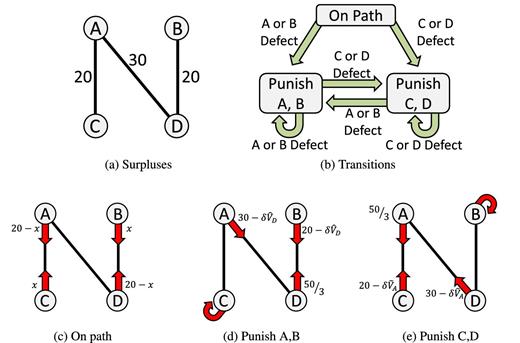
Constructing an EPE for Game 30. Panel (b) shows the transitions between states when players deviate from the prescribed play, whereas panels (c)–(e) show how players play in each state. Red arrows indicate whom a player offers to if selected as the proposer; and the numbers next to the arrows indicate the payoffs that the offering players will keep.

We construct off-path punishments that are credible and create the appropriate incentives for players to remain on path. This is achieved by defining two different punishment states, prescribing play in each of these states and a rule for transitioning between them in a way that creates the appropriate incentives. These transitions are such that they occur only if someone deviates from their prescribed strategy, in which case the person who initiated the deviation is punished by moving to the state that punishes her. Importantly, these transitions also reward all the players with whom the punished player is linked. These transitions are illustrated in panel (b) of Figure B.1.

To show that the punishments are credible, suppose we are in the Punish A, B state. If everyone plays as prescribed, we remain in this state and the payoffs of the players are given by the following value functions:

$$\begin{eqnarray} \widehat{V}_{\rm A}&= \frac{1}{4}\left(30-\delta \widehat{V}_{\rm D}+2 \delta W(\delta )+\delta \widehat{V}_{\rm A}\right)=\frac{30-\delta \widehat{V}_{\rm D}+2 \delta W(\delta )}{4-\delta }\rightarrow 11\frac{1}{9}, \\ \widehat{V}_{\rm B}&= \frac{1}{4}\left(20-\delta \widehat{V}_{\rm D} +3\frac{1}{3}+\delta \widehat{V}_{\rm B}\right)=\frac{20-\delta \widehat{V}_{\rm D}+3\frac{1}{3}}{4-\delta }\rightarrow 2\frac{2}{9}, \\ \widehat{V}_{\rm C}&= \frac{1}{4}\left(\delta \widehat{V}_{\rm C}+2\,W(\delta )\right)=\frac{2\,W(\delta )}{4-\delta }\rightarrow 6\frac{2}{3}, \\ \widehat{V}_{\rm D}&= \frac{1}{4}\left(16\frac{2}{3}+3\delta \widehat{V}_{\rm D}\right)=\frac{16\frac{2}{3}}{4-3\delta }\rightarrow 16\frac{2}{3}. \end{eqnarray}$$

By symmetry, the Punish C, D state value functions of the players are

$$\begin{eqnarray} \widetilde{V}_{\rm A}&= \frac{16 \frac{2}{3}}{4-3\delta }\rightarrow 16 \frac{2}{3}, \\ \widetilde{V}_{\rm B}&= \frac{2\,W(\delta )}{4-\delta }\rightarrow 6\frac{2}{3}, \\ \widetilde{V}_{\rm C}&= \frac{20-\delta \widehat{V}_{\rm D}+3\frac{1}{3}}{4-\delta }\rightarrow 2\frac{2}{9}, \\ \widetilde{V}_{\rm D}&= \frac{30-\delta \widehat{V}_{\rm D}+2\,W(\delta )}{4-\delta }\rightarrow 11 \frac{1}{9}. \end{eqnarray}$$

Consider now the deviations available to the players in the Punish A, B state. First, suppose that A deviates and offers D less than |$\delta \widehat{V}_{\rm D}$|⁠. By rejecting the offer, D ensures that we remain in the same state and that he will receive, in expectation, |$\delta \widehat{V}_{\rm D}$|⁠. Alternatively, A may delay, in which case A receives |$\delta \widehat{V}_{\rm A}<30-\delta \widehat{V}_{\rm D}$|⁠. Finally, A could offer to C. C would accept anything greater than |$\delta \widehat{V}_{\rm C}$| and reject anything less, because we would remain in the Punish A, B state. Thus, A must offer C a limit payoff of |$6\frac{2}{3}$|⁠, leaving A with |$13\frac{1}{3}\le 30-16\frac{2}{3}=13 \frac{1}{3}$|⁠.⁴⁹ The alternative deviations available to B are to offer D less than |$\delta \widehat{V}_{\rm D}$|⁠, which D would reject, leaving B with |$2\frac{1}{3}<3\frac{1}{3}$|⁠, or to delay, which would also leave B with |$2\frac{1}{3}<3\frac{1}{3}$|⁠. The only deviation available to C is to make an offer to A. As rejecting C’s offer will result in a switch of states, A would accept only a limit payoff which is weakly greater than |$16\frac{2}{3}$|⁠, leaving C with |$3\frac{1}{3}<6\frac{2}{3}$|⁠. Finally, D could deviate. As a deviation by D would result in a switch of states if rejected, for an off-path offer to be accepted D must offer B at least |$6\frac{2}{3}$| in the limit, or A at least |$16\frac{2}{3}$| in the limit. Both deviations are thus unprofitable. Finally, as delay would also result in a switch of states, that alternative is unprofitable for D as well. This covers all the possible deviations from the Punish A, B state. By symmetry, there are no profitable deviations from the Punish C, D state.

For these punishments to be effective, in the on-path state C and B must be required to accept only offers, in the limit, of weakly more than |$2\frac{2}{9}$|⁠, or to make offers that leave them with at least |$2\frac{2}{9}$|⁠. Similarly, A and D must be required to accept only offers of weakly more than |$11\frac{1}{9}$| in the limit, or to make offers that leave them with at least |$11\frac{1}{9}$| in the limit. Thus, for any |$x\in (2\frac{2}{9},8\frac{8}{9}),$| there exists an EPE. This places bounds on the offers that can be supported when all the players are active. In the subgame reached once an efficient pair has exited, the remaining players get limit payoffs of 10. Thus, the weak players will have limit expected payoffs in the range |$(6\frac{1}{9},9\frac{4}{9})$|⁠, whereas the strong players will have limit expected payoffs in the range |$(10\frac{5}{9},13\frac{8}{9})$|⁠.

The construction we use to find an EPE for Game 30 also works for Game 25. In that case, in the Punish A, B state we would need to make A offer D no more than |$11\frac{2}{3}$|⁠, leaving A with |$13\frac{1}{3}$|⁠, so that A does not want to deviate and, instead, offer to C. As A offers D his continuation value, this implies that |$V_{\rm D}=11\frac{2}{3}$|⁠, which means that B also offers |$11\frac{2}{3}$| to D and that D offers |$8\frac{1}{3}$| to B. This gives a limit payoff to B of |$V_{\rm B}=5\frac{5}{9}$|⁠. As before, C’s limit payoff is |$V_{\rm D}=6\frac{2}{3}$|⁠. Finally, A’s limit payoff is |$11\frac{1}{9}$|⁠. Given these strategies and limit payoffs, it can be verified that all the incentive constraints are satisfied. Thus, there is an EPE for any |$x\in (5\frac{5}{9},8\frac{8}{9})$|⁠. As limit payoffs in the subgame are again 10, weak players have limit expected payoffs in the range |$(7\frac{7}{9},9\frac{4}{9}),$| whereas strong players have limit payoffs in the range |$(10\frac{5}{9},12\frac{2}{9})$|⁠.

Although for Game 15 the MPE is efficient, this construction cannot be used in this Game to extend the payoffs that can be supported in an EPE. The intuition is that the strong players can always guarantee themselves 10 by ignoring their link, whereas they cannot use this link to get more than 10 because the threat of matching inefficiently and receiving an average payoff of 7.5 is not credible. To see what specifically goes wrong with the construction, let x be the amount player D asks to keep when making an offer to B in the Punish A, B state. Note that C’s limit continuation value is still |$6\frac{2}{3}$| and that C is required to delay. If C deviates and does not delay, then C is punished by moving to the Punish C, D state. In that case, C gets the same limit payoff that B gets in the Punish A, B state. That limit payoff is |$\frac{2}{3}(20-x)$|⁠, so we require that x ≥ 10. However, in that case, the limit payoff of A is |$\frac{1}{3}(15-x)+\frac{2}{3}(10)\le 8\frac{1}{3}$|⁠. But this means that A has an incentive to deviate and delay. This deviation does not change the state (as we are already in the Punish A, B state), but does mean that B and D will match first for sure, leaving A with a limit payoff of 10.

Appendix C: Cooperative Theories

With unstructured bargaining, efficiency-enhancing norms could emerge to the mutual benefit of everyone. The participants have much more freedom to reach implicit agreements that exploit inefficiencies for their mutual gain. This logic is present in several solution concepts from cooperative game theory, and with unstructured bargaining, we might expect their predictions to be borne out. To guide our experiment, we consider two such theories: (i) an extension of Nash bargaining, where the disagreement points are defined endogenously by the market; and (ii) the midpoint of the core.⁵⁰

The first solution concept we consider is Symmetric Pairwise Bargained (SPB) outcomes, first developed by Rochford (1984) and independently discovered by Kleinberg and Tardos (2008). This approach extends Nash bargaining to networks. A player’s disagreement payoff is the surplus they could obtain by just enticing someone else to match with them. Given these disagreement payoffs, each of the two players reaching an agreement gets their disagreement payoff plus an equal share of the remaining surplus. Of course, the disagreement payoff for a given player depends on the agreements others reach, and so the solution boils down to finding a fixed point of a large system of equations. We derive predictions for Games 15, 25, and 30 in Section E.1 in the Online Appendix. These predictions coincide with the predictions of three other cooperative solution concepts, kernel, prekernel, and nucleolus.

Our next cooperative theory is an alternative refinement of the core. The core comprises the set of bargaining outcomes that allocate the surplus generated by matching such that there is no coalition of players that could find a match among themselves, and then allocate that surplus in a way that makes them all better off. Shapley and Shubik (1972) show that there are no profitable coalitional deviations if and only if there are no profitable pairwise deviations, which just requires that for all worker–firm pairs the sum of their payoffs is weakly greater than the surplus they could generate by matching with each other. This implies that the match implemented must be efficient. It also follows from results by Shapley and Shubik (1972) that there is a midpoint of the core in which two players reaching an agreement receive their worst possible core payoff for sure, and then split the remaining surplus equally.⁵¹ In an NTU environment, Echenique and Yariv (2013) experimentally find that the median stable match is reached. For the markets we consider, the midpoint of the core corresponds to the TU median stable matching (Schwarz and Yenmez 2011). These predictions are derived in Section E.2 in the Online Appendix and reported in Table C.1.

Table C.1.

Theoretical predictions about final matches.

	Game 15			Game 25			Game 30
	eff.(%)	B (C)	A (D)	eff.(%)	B (C)	A (D)	eff.(%)	B (C)	A (D)
SPB	100	8.3	11.7	100	5	15	100	3.3	16.7
Core	100	[0, 20]	[0, 20]	100	[0, 15]	[5, 20]	100	[0, 10]	[10, 20]
Core midpoint	100	10	10	100	7.5	12.5	100	5	15

Footnotes

1.

See Rogerson, Shimer, and Wright (2005) and Rogerson and Shimer (2011) for surveys of the search literature. Informational frictions are studied in Calvó-Armengol and Jackson (2004), among others.

2.

Specifically, assuming that workers are vertically differentiated, firms are vertically differentiated, and surpluses are either supermodular or submodular. Under these assumptions, the welfare loss from inefficient matching can be identified.

3.

Many labor markets are characterized by heterogeneous surpluses so that it matters which worker is employed by which firm. We expect, however, that getting the “right” worker to be employed by the “right” firm is likely to matter more in high-skill labor markets. These markets are also characterized by wages being negotiated (Hall and Krueger 2012) and are economically important: The top 10% of earners accounted for 45% of overall income and for 68% of federal income tax receipts in the United States in 2011 (http://www.heritage.org).

4.

See Kessler and Vesterlund (2015) for a recent discussion regarding the external validity of laboratory experiments.

5.

The tradition of theory-based experiments goes back to the market experiments of Vernon Smith and Charles Plott, which had a profound effect on our understanding of the functioning of markets and the performance of economic institutions.

6.

See Roth (1987) for an overview of experimental work on coalition bargaining, which was mostly concerned with testing cooperative game theory concepts, Roth (1995) for a survey of early experiments exploring noncooperative theories of bargaining, and Palfrey (2016) for a recent survey of multilateral bargaining games.

7.

For an experimental study of one-sided matching markets with NTU, see Molis (2010). For studies with a more rigid bargaining structure, such as the one in which one side of the market makes offers to the other side but not vice versa, see Haruvy and Ünver (2007) and Niederle and Roth (2009). Finally, see Kagel (2000) and Featherstone and Mayefsky (2015), who study unravelling and the transition between a decentralized market and a centralized clearinghouse.

8.

These matching procedures range from the free-agency system similar to the problem of matching baseball players to teams to the simultaneous bid mechanism, in which participants on each side of the market simultaneously submit the maximum amount they are willing to pay to be matched to each participant on the other side of the market.

9.

See also Gale and Kariv (2009) and Choi, Galeotti, and Goyal (2014) for a study of trading in networks with intermediaries, implemented through a simultaneous bid-ask protocol and posted prices, respectively.

10.

Perhaps the closest papers to ours are Bienenstock and Bonacich (1993) and Skvoretz and Willer (1993). Both consider a variety of theories, including some from cooperative game theory.

11.

The MPE are motivated in Maskin and Tirole (2001), and have been theoretically justified on complexity grounds as those selected when there is a second-order lexicographic preference for simple strategies (Sabourian 2004).

12.

For example, we can calculate the expected payoff of C as follows: With probability 0.5, A or D proposes and C gets 0; with probability 0.25, B proposes and reaches an agreement with D, leaving C to get 10 from bargaining bilaterally with A; and with probability 0.25, C proposes and gets 20 less the minimum offer A will accept.

13.

They show that by cleverly constructing punishments, an EPE always exists in markets where the gains from trade are either 1 or 0.

14.

The reason is that in any EPE either B or C will be left to bargain bilaterally with their efficient partner, thus receiving a limit payoff of 10.

15.

Experiments II and III are not amenable to a noncooperative analysis. For example, in Experiment II, the corresponding noncooperative game would be in continuous time with an endogenous ordering and timing of moves. In such settings, these cooperative solution concepts may be particularly relevant.

16.

If the market outcome was not efficient, then the grand coalition would be able to form and implement the match that maximized total surplus, and then redistribute this surplus in a way that made everyone better off. Thus, only efficient market outcomes are robust to coalitional deviations, and, hence, by Shapley and Shubik’s result, only efficient market outcomes are robust to pairwise deviations.

17.

This is the transferable utility (TU) equivalent to median stable matches in an non-transferable utility (NTU) environment (Schwarz and Yenmez 2011), which has received some experimental support in NTU matching experiments (Echenique and Yariv 2013).

18.

The Shapley value makes unappealing predictions in matching markets, and so we do not consider it. For example, with one worker and two firms, the Shapley value will typically require the firm that ends up unmatched to receive a transfer of surplus from the matched pair.

19.

We decided to look at these predictions ex post, after considering the performance of the theories quantitatively and qualitatively in other dimensions.

20.

We took the decision to look at these more nuanced predictions of the MPE ex post, after we found substantial rates of mismatch.

21.

We decided to look at predictions regarding strategies ex post, after analyzing the performance of the theories in the other dimensions.

22.

The software for the experiment was developed from the open source Multistage package, available for download at http://software.ssel.caltech.edu/.

23.

In Online Appendix Section G, we report the location at which each session was conducted and compare the behavior of subjects across the two laboratories. Our data suggest that subjects’ behavior is similar across these two subject pools.

24.

A total of 40 subjects participated in Game 15 treatment, 68 subjects participated in Game 25 treatment, and 68 subjects participated in Game 30 treatment.

25.

In other words, this rule means the game ends if there are no possible matches between any two players who are both still actively bargaining (by making proposals). This includes the situation in which the two strong players (players with two links) match with each other and exit the market leaving the two weak players unmatched as well as the situation in which all four players are matched (each weak player is matched with a strong player).

26.

The list of questions and the screenshots of the game are also presented in Online Appendix Section I.

27.

Random termination was very rare: About 6% of games in all treatments of Experiment I ended because of random termination.

28.

In contrast, in Game 15 the MPE predicts that the network position of the first mover plays no role as all outcomes are expected to be efficient.

29.

Note that when an inefficient match is reached, weak players must receive a payoff of 0 and the average payoff of a strong player must be 12.5 in Game 25 and 15 in Game 30.

30.

Only the payoffs of strong players are shown, but the expected payoffs of weak players conditional on reaching the efficient match are 20 less the payoff of the strong players conditional on reaching the efficient match.

31.

Indeed, any subject who proposed two different amounts to the player in the same network position conditional on the same market composition cannot be playing a Markovian strategy.

32.

We also run a hypothesis test with a null hypothesis of β₁ = β₂ and an alternative hypothesis of β₁ > β₂ and find evidence to reject the null (p = 0.0002). This provides evidence that subjects in strong positions are more likely to make efficient proposals in Game 25 than in Game 30.

33.

Figure D.31 in Online Appendix D.3 depicts box plots of average absolute differences between amounts offered and those predicted by the MPE both in the first and in the second halves of the experiment in order to document how subjects’ behavior changes as they gain experience with the game.

34.

These frequencies are even higher in the first five repetitions of a game: 65% of weak players demand equal split of surplus at least once in Game 25 and 81% of weak players do so in Game 30. The average frequency with which an equal split is demanded is 61% in both games among the players who demand an equal split at least once.

35.

Figures D.32 and D.33 in Online Appendix D.3 depict the acceptance/rejection behavior of our responders in each of the games in the first and the second halves of the experiment, respectively.

36.

Of the 10 offers in which we observe weak players being offered less than 6.45, 9 are rejected.

37.

In particular, in Game 25, only 50% of offers made by weak players who were first movers were accepted, whereas this fraction is 70% for strong players who were selected to be first movers. Similarly, in Game 30, only 53% of offers made by weak players who were first movers were accepted, whereas this fraction is 87% for strong players who were first movers.

38.

These patterns cannot be explained by the rates at which strong and weak players are selected to be the proposer. We find no statistical difference between these rates in any treatment.

39.

A closely related finding is that the players in strong positions are typically not willing to accept the perfectly equitable and efficient outcome, and instead want to exploit their strong positions. This is consistent with findings in Weg et al. (1990) and Kagel, Kim, and Moser (1996).

40.

This explanation is also consistent with the outside option principle from bargaining theory. Consider the inefficiencies we would expect to find were two players to bargain bilaterally, but with one of them having a long-lived outside option. In this case, the “outside option principle” predicts that the two players should reach an agreement with probability 1 such that there is no mismatch, and, if the outside option is binding, the player with the binding outside option should receive a payoff equal to its value. Experimental support for precisely this is presented in Binmore, Shaked, and Sutton (1989). The reason the outside option principle does not apply to Experiment I is that it is based on outside options always being available. When alternative matches can be lost, because others exit the market, they do not act like outside options. If, instead, players did not exit the market, and could renege on their current deals, then the same alternative matches would always be available. In this case, the logic of the outside option principle seems more applicable.

41.

See, for example, Avery et al. (2001).

42.

Specifically, to make an offer a subject has to click on the ID letter of the subject she wants to receive the offer, and to type in the amount that she proposes to keep for herself; the remaining portion of the surplus the match would generate is allocated to the recipient. The offer then immediately appears in the column OFFERS YOU PROPOSED on the screen of the proposer and in the column OFFERS PROPOSED BY OTHERS on the screens of all the subjects still in the market. By clicking on a button, the recipient can accept the offer at any time until it is withdrawn.

43.

In this section, we briefly summarize the main features of Experiment III and refer the reader to Online Appendix Section K, in which we present instructions, the screenshots, and the quiz for this experiment.

44.

A total of 40 subjects participated in the Game 15 treatment, 60 subjects in the Game 25 treatment, and 56 subjects in the Game 30 treatment.

45.

Specifically, when a player reaches an agreement with another player, the button responsible for submitting offers is disabled and the only active button on the screen of a matched player is the “Do Nothing” button, which she has to press in every round thereafter. We chose such a design in order to keep all the subjects engaged and focused on a game, irrespective of the order in which they formed matches.

46.

In other words, the button responsible for submitting offers is never disabled no matter whether a player is matched with another player or not.

47.

The regression presented in Table 15 also reveals that in Game 15 efficiency is significantly lower in Experiment III than in Experiment I. Whereas in Experiment I there are no inefficient matches, in Experiment III there are inefficient matches in about 4% of cases. We do not view this as substantial.

48.

Based on the estimated coefficients presented in Regression (12), we reject both H0: β₀ = 1.00 in favor of H1: β₀ < 1 with p < 0.0001 and H0: β₀ + β₁ = 1.00 in favor of H1: β₀ + β₁ < 1 with p = 0.0024. Moreover, comparing efficiency levels in Game 30 obtained in Experiments II and III, we find that this difference is statistically significant at the 10% level (p = 0.0895).

49.

This inequality would become strict, whereas the others remain satisfied, were the offer D makes to B to be increased slightly. We make this incentive constraint tight to make the punishment as harsh as possible so that we can find the full range of payoffs that can be supported.

50.

We do not consider the Shapley value or related concepts. The Shapley value makes predictions that can be infeasible in our setting when each matched pair of players is required to split between themselves the surplus they generate. For example, if there is one worker and two firms and all matches generate a positive surplus, then the Shapley value requires that all players receive strictly positive payoffs.

51.

These payoffs are special cases of Corominas-Bosch (2004) and Elliott (2015), whereas Kranton and Minehart (2001) use a related selection.