


Abstract
According to Dr. Michael Laposata, the medical specialty that nearly every practicing physician relies on every day, for which training in many medical schools is limited to no more than a scattered few lectures throughout the entire curriculum, is “laboratory medicine.” The importance of understanding the principles for selecting and ordering the most rational laboratory test(s) on a specific patient is heightened in the current age of managed care, medical necessity, and outcome-oriented medicine. The days of a “shotgun approach” to ordering laboratory tests has, of necessity, been replaced by a “rifle” (or targeted) approach based on an understanding of the test’s diagnostic performance and the major “legitimate” reasons for ordering a laboratory test. Such an understanding is critical to good laboratory practice and patient outcomes.
The purpose of this CE Update is to discuss the laboratory testing cycle and its importance in diagnostic decision making. This discussion will begin with some general comments about approaches to ordering clinical laboratory tests, followed by “real-world” examples to illustrate these approaches. We will then review the important diagnostic performance characteristics of laboratory tests, how they are calculated, and a principal tool (ie, receiver-operator characteristic [ROC] curves) used to assess the diagnostic accuracy of a laboratory test at specific cutoff values for the test. We will then discuss how laboratory tests are interpreted using a reference interval and its limitations, followed by some brief remarks about the concepts critical difference and neural network.
The “Laboratory Testing Cycle”
The “laboratory testing cycle” (Figure 1) consists of all steps between the time when a clinician thinks about and orders a laboratory test and the time the appropriate patient’s sample for testing is obtained (eg, a blood specimen taken from an antecubital vein) and the results of the testing are returned to the clinician (often called the “vein-to-brain” turnaround time [TAT] of test results). This cycle consists of 3 phases: preanalytic, analytic, and post-analytic (Figure 1).
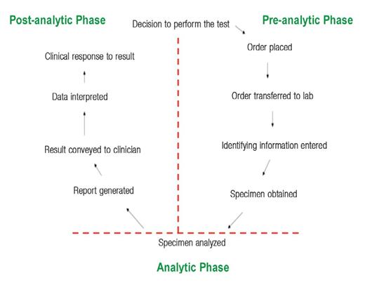
The “Laboratory Testing Cycle.”
Common causes of preanalytical errors include a variety of factors, many of which are summarized in Table 1.
Examples of Common Causes of Preanalytical Error
| Biological |
| Age |
| Sex |
| Race (Blacks vs. Caucasians) |
| Behavioral |
| Diet |
| Obesity |
| Smoking |
| Alcohol intake |
| Caffeine intake |
| Exercise |
| Stress |
| Clinical (20Alterations) |
| Diseases: |
| Hypothyroidism |
| Insulin-dependent diabetes mellitus |
| Nephrotic syndrome/chronic renal failure |
| Biliary tract obstruction |
| Acute myocardial infarction |
| Drug Therapy: |
| Diuretics |
| Propanolol |
| Oral contraceptives with high [progestin] |
| Oral contraceptives with high [estrogen] |
| Prednisolone |
| Cyclosporine |
| Pregnancy |
| Specimen Collection & Handling |
| Specimen obtained from wrong patient* |
| Specimen mix-up* |
| Nonfasting vs. fasting (12 h) |
| Anticoagulant: |
| EDTA |
| Heparin |
| Capillary vs. venous blood |
| Hemoconcentration (eg, use of a tourniquet) |
| Specimen storage (@ 0–4 °C for up to 4 days) |
Common sources of preanalytical error; however, frequency decreasing with advent of better quality assurance (QA) procedures to ensure positive patient ID and labeling of specimen tubes.
Analytical errors are of 2 types: random or systematic, and systematic errors can be subdivided further into constant or proportional error. Random errors can be caused by timing, temperature, or pipetting variations that occur randomly during the measurement process and are independent of the operator performing the measurement. Systematic error is caused frequently by a time-dependent change in instrument calibration that causes the calibration curve to shift its position and alter the accuracy and/or precision (reproducibility) of the quantitative results obtained using this curve.
Post-analytical errors include such mistakes as transcription errors (eg, an accurate and reliable result reported on the wrong patient, using the wrong value, and/or with the wrong units [eg, mg/L instead of mg/day]).
The results of a relatively recent article on the sources of laboratory errors in stat testing, which should be very gratifying to laboratorians, has shown that analytical sources of error occurred least frequently (15%) while preanalytical errors occurred most frequently (62%) (Figure 1A).1
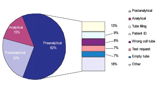
The top 5 causes of preanalytical errors were:1
Specimen collection tube not filled properly.
Patient ID error.
Inappropriate specimen collection tube/container.
Test request error.
Empty collection tube.
Although 75.6% of all sources (preanalytical, analytical, or post-analytical) of laboratory errors had no effect on patient outcomes, ~25% had a negative impact, indicating much opportunity to reduce laboratory errors to Six Sigma levels (ie, < 3.4 errors/1 million opportunities) or near perfection.1,2
Diagnostic Decision Making
The use of clinical laboratory test results in diagnostic decision making is an integral part of clinical medicine. The menu of laboratory tests available to clinicians constitutes an impressive array that has expanded exponentially since 1920 when Folin and Wu devised the first useful test for the quantification of serum glucose concentration.3 The current list of tests offered by one major reference laboratory includes nearly 3,000 analytes, which does not include the additional array of more commonly ordered tests (eg, complete blood count [CBC], electrolytes [sodium, potassium, chloride, carbon dioxide], thyroid stimulating hormone [TSH], glucose, etc.) routinely performed on site by most hospital-based clinical laboratories. Despite this ever-expanding plethora of useful and reliable clinical laboratory tests for diagnosing and monitoring the myriad of diseases effecting mankind, the recent emphasis on reducing health care costs and the emergence of managed care organizations led to efforts to reduce the abuse (over-ordering) and misuse (eg, ordering the right test for the wrong purpose or vice versa) of these tests.
Medical Necessity
As private health maintenance organizations (HMOs) and government-sponsored agencies (eg, Department of Health and Human Services [DHHS] and the Centers for Medicare and Medicaid Services [CMS]) seek to provide quality medicine cost effectively, reduction in the ordering of “unnecessary” laboratory tests has become a favorite target of these efforts. The critical question facing physicians, however, is: What constitutes an unnecessary laboratory test? In the current climate of business-oriented medicine, the answer should not be: Any test for which reimbursement by a payer (eg, Medicare) is likely to be denied. The correct answer is: Any test for which the results are not likely to be “medically necessary” in the appropriate management of the patient’s medical condition. Thus, it is incumbent upon physicians and laboratorians to understand which laboratory tests are appropriate to order in the diagnosis and follow up of a patient’s medical condition.
Questions to Ask Before Ordering a Laboratory Test
An understanding of which laboratory tests are appropriate to order in the diagnosis and follow up of a patient’s medical condition should include prior consideration of the answers to the following questions:4
Why is the test being ordered?
What are the consequences of not ordering the test?
How good is the test in discriminating between health versus disease?
How are the test results interpreted?
How will the test results influence patient management and outcome?
The answers to these questions are critical to the optimal selection and cost-effective use of laboratory tests likely to benefit patient management. A major misconception among clinicians is the feeling that a laboratory test is more objective than a patient’s history and physical examination. Nevertheless, it is widely accepted that the judicious use of laboratory tests, coupled with thoughtful interpretation of the results of these tests, can contribute significantly to diagnostic decision making and patient management.
Reasons for Ordering a Laboratory Test
There are 4 major legitimate reasons for ordering a laboratory test:4
Diagnosis (to rule in or rule out a diagnosis).
Monitoring (eg, the effect of drug therapy).
Screening (eg, for congenital hypothyroidism via neonatal thyroxine testing).
Research (to understand the pathophysiology of a particular disease process).
Approaches for Establishing a Diagnosis Based on Laboratory Test Results
The principal approaches for establishing a diagnosis based on laboratory test results include:4
Hypothesis deduction.
Pattern recognition.
Medical algorithms.
Rifle versus shotgun approach.
Hypothesis deduction involves establishing a differential diagnosis based on the patient’s history, including family, social, and drug history, and physical exam findings, followed by the selection of laboratory tests that are the most likely to confirm (ie, allow the clinician to deduce) a diagnosis on the list of differential diagnoses.
Example 1Hypothesis deduction approach to laboratory test ordering: A 4-year-old child presents to the emergency room (ER) with an upper respiratory tract infection (URI), fever (102.2°F), and generalized seizures lasting 2 min. The clinician establishes a differential diagnosis of meningitis versus febrile seizures and deduces that the most appropriate laboratory tests to discriminate between these possibilities are the following tests performed on cerebrospinal fluid (CSF) from a spinal tap:
White blood cell (WBC) and red blood cell (RBC) counts.
Total protein.
Glucose.
Gram stain.
Bacterial, viral, and/or fungal cultures.
Rapid polymerase chain reaction (PCR) assay for a meningococcus-specific insertion sequence (IS).
All results for these tests were either “normal,” “negative,” or “no growth” (cultures), supporting a diagnosis of febrile seizure over bacterial, viral, or fungal meningitis.
Pattern recognition involves comparing the patient’s pattern of results for several laboratory tests that have been determined previously to provide excellent power in discriminating between various competing and/or closely related diagnoses (Table 2). The pattern of laboratory test results shown for the pregnant “Patient” in Table 2 most closely match those consistent with a diagnosis of idiopathic thrombocytopenic purpura (ITP), rather than other possible causes of pregnancy-associated thrombocytopenia: gestational thrombocytopenic (GTP); thrombotic thrombocytopenia (TTP); hemolytic uremic syndrome (HUS); disseminated intravascular coagulation (DIC); or, (syndrome of) hemolysis, elevated liver enzymes, and low platelet count (HELLP).
Example of Pattern Recognition Approach to Diagnosis
PT, prothrombin time; APTT, activated partial thromboplastin time; AST, aspartate aminotransferase; ALT, alanine aminotransferase; LD, lactate dehydrogenase; BUN, blood urea nitrogen; RBC, red blood cell; N, normal; LN, low-normal; ↓, decreased; ↑, increased, ↑↑↑, markedly increased; +/−, may be positive or negative; −, negative
The Effect of Disease Prevalence on the Positive (PPV) and Negative Predictive Value (NPV) of a Laboratory Testa
| Disease Prevalence, % | PPV, % | NPV, % |
|---|---|---|
| 0.1 | 1.9 | 99.9 |
| 1 | 16.1 | 99.9 |
| 10 | 67.9 | 99.4 |
| 50 | 95.0 | 95.0 |
| 100 | 100.0 | n.a. |
| Disease Prevalence, % | PPV, % | NPV, % |
|---|---|---|
| 0.1 | 1.9 | 99.9 |
| 1 | 16.1 | 99.9 |
| 10 | 67.9 | 99.4 |
| 50 | 95.0 | 95.0 |
| 100 | 100.0 | n.a. |
In this example, the test is assigned 95% diagnostic specificity and 95% diagnostic sensitivity. n.a., not applicable.
Medical algorithms (or “decision trees”) are particularly useful in establishing a diagnosis based, in part, on information obtained from ordering the most appropriate (ie, necessary) laboratory tests. Such algorithms (cf., Figures 2 and 2.1) are advantageous because they:
are logical and sequential;
can be automated using a computer to achieve rapid turnaround time of results for tests included in the algorithm;
maximize a clinician’s efficiency;
minimize the ordering of unnecessary laboratory tests;
can be used by ancillary medical personnel (eg, physician assistants and nurse practitioners) assisting physicians;
can be easily updated with improved strategies for diagnostic decision making as new and better tests become available; and
are incorporated into software programs that are relatively inexpensive to purchase and use.
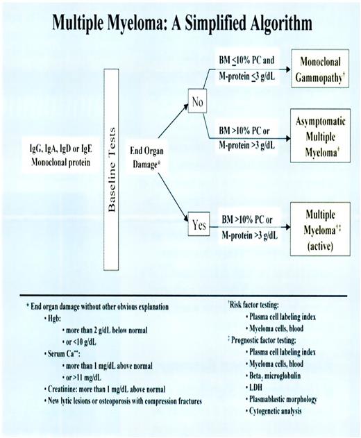
Simplified algorithm for the diagnosis of a monoclonal gammopthy versus asymptomatic multiple myeloma versus active multiple myeloma (Source: Mayo Communique. 2002;27:2).
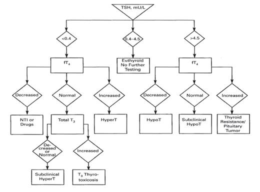
Algorithm for identifying individuals with thyroid disorders based on TSH level. TSH, thyroid-stimulating hormone; fT4, free thyroxine; NTI, nonthyroid illness; T3, trilodothyronine; HyperT, hyperthyroidism; HypoT, hypothyroidism.
The rifle versus shotgun approach to laboratory test ordering relates to ordering specific laboratory tests based on an assessment of their diagnostic accuracy and predictive value in identifying a particular disease (ie, using a “rifle” to hit the bulls-eye representing the correct diagnosis) versus indiscriminate ordering of a large number of laboratory tests that may or may not have adequate diagnostic accuracy and predictive value in identifying a particular disease (ie, using a “shotgun” to hit the target, which is likely to create a pattern of shots on the target, none of which may hit the bulls-eye). Ordering the following 20 laboratory (and other) tests on a 4-year-old child with signs and symptoms of an upper respiratory tract infection, fever (102.2 °F), and generalized seizure lasting 2 min represents a shotgun—and very expensive—approach to arriving at a diagnosis:
WBC count w/differential
Quantitative immunoglobulins (IgG, IgA, IgM)
Erythrocyte sedimentation rate (ESR)
Quantitative alpha-1-antitrypsin (AAT) level
Retic count
Arterial blood gasses (ABGs)
Throat culture
Sweat chloride
Nasal smear for eosinophils
Nasopharyngeal culture for pertussis infection
Viral cultures
Stool exam for ova and parasites (O & P)
Urinalysis
Purified protein derivative (tuberculin) (PPD)/trichophyton/cocci skin tests
Electrolytes
Glucose
Total bilirubin
Aspartate aminotransferase (AST)
Alanine aminotransferase (ALT)
Chest X-ray (×3)
Electrocardiogram (ECG)
A rifle approach would involve ordering only those laboratory tests useful in discriminating between the diseases constituting the differential diagnosis (ie, meningitis or febrile seizure) as indicated in Example 1 above (ie, the 7 to 9 “targeted” tests on CSF).
Clinical Performance Characteristics of Laboratory Tests
Because the clinical performance characteristics of all laboratory tests differ with respect to their diagnostic accuracy (ie, sensitivity and specificity), the selection of the appropriate laboratory test to order will vary depending on the purpose for which the test is to be used. Before considering this aspect of the selection of laboratory tests, we must first understand the terms that describe their diagnostic performance. These terms include prevalence, sensitivity, specificity, efficiency, and predictive value. To illustrate the mathematical calculation of values for each of these parameters, consider the example given below:4,5
Example 2 The laboratory test, prostate-specific antigen (PSA), was studied with regard to its ability to discriminate patients with prostate cancer (PCa) from those without PCa. This test was performed on 10,000 men, 200 of whom have biopsy-proven prostate cancer. Using this information, a 2 x 2 table can be constructed as shown below:
| No. of Men With PCa | No. of Men Without PCa | Total | |
|---|---|---|---|
| No. of men with positivea | 160 | 6,860 | 7,020 |
| PSA test | (TP) | (FP) | |
| No. of men with negativeb | 40 | 2,940 | 2,980 |
| PSA test | (FN) | (TN) | |
| Total | 200 | 9,800 | 10,000 |
| No. of Men With PCa | No. of Men Without PCa | Total | |
|---|---|---|---|
| No. of men with positivea | 160 | 6,860 | 7,020 |
| PSA test | (TP) | (FP) | |
| No. of men with negativeb | 40 | 2,940 | 2,980 |
| PSA test | (FN) | (TN) | |
| Total | 200 | 9,800 | 10,000 |
Positive PSA test = men with a serum PSA concentration ≥ 4.0 ng/mL
Negative PSA test = men with a serum PSA concentration < 4.0 ng/mL
| No. of Men With PCa | No. of Men Without PCa | Total | |
|---|---|---|---|
| No. of men with positivea | 160 | 6,860 | 7,020 |
| PSA test | (TP) | (FP) | |
| No. of men with negativeb | 40 | 2,940 | 2,980 |
| PSA test | (FN) | (TN) | |
| Total | 200 | 9,800 | 10,000 |
| No. of Men With PCa | No. of Men Without PCa | Total | |
|---|---|---|---|
| No. of men with positivea | 160 | 6,860 | 7,020 |
| PSA test | (TP) | (FP) | |
| No. of men with negativeb | 40 | 2,940 | 2,980 |
| PSA test | (FN) | (TN) | |
| Total | 200 | 9,800 | 10,000 |
Positive PSA test = men with a serum PSA concentration ≥ 4.0 ng/mL
Negative PSA test = men with a serum PSA concentration < 4.0 ng/mL
From this data, the values for prevalence, sensitivity, specificity, efficiency, positive predictive value (PPV), and negative predictive value (NPV) can be determined:
Prevalence (p) = No. of individuals with disease/No. of individuals in population to be tested = 200/10,000 = 0.020 = 2.0%
Sensitivity = percentage of individuals with disease who have a positive test result = No. of true-positives/(No. of true-positives + No. of false-negatives) or TP/(TP + FN) = 160/(160 + 40) = 160/200 = 0.800 = 80%
Specificity = percentage of individuals without disease who have a negative test result = No. of true-negatives/(No. of true-negatives + No. of false-positives) or TN/(TN + FP) = 2,940/(2,940 + 6,860) = 2,940/9,800 = 0.30 = 30%
Efficiency =percentage of individuals correctly classified by test results as being either positive or negative for the disease = (TP + TN)/(TP + FP + FN + TN) = (160 + 2,940)/10,000 = 3,100/10,000 = 0.31 = 31%
Positive Predictive Value (PPV) = percentage of individuals with a positive test result who truly have the disease = TP/(TP + FP) = 160/(160 + 6,860) = 160/7,020 = 0.023 = 2.3%, or PPV = (sensitivity)(p)/[(sensitivity)(p) + (1 - specificity) (1 - p) = (0.8)(0.02/[(0.8)(0.02) + (1 - 0.3) (1 - 0.02)] = 0.016/[0.016 + (0.7)(0.98)] = 0.016/[0.016 + 0.686] = 0.016/0.702 = 0.023 = 2.3%
Negative Predictive Value (NPV) = percentage of individuals with a negative test result who do not have the disease = TN/(TN + FN) = 2,940/(2,940 + 40) = 2,940/2,980 = 0.987 = 98.7%, or NPV =(specificity)(1 - p)/[(specificity) (1 - p) + (1 - sensitivity)(p)] = (0.3)(1 - 0.02)/[(0.3)(1 - 0.02) + (1 - 0.8)(0.02)] = 0.294/0.298 = 0.987 = 98.7%
Sum of Sensitivity and Specificity = 80 + 30 = 110 (Note: In general, a useful laboratory test will have a sum >170)
It is important to note that any test with a sensitivity = 50% and a specificity = 50% is no better than a coin toss in deciding whether or not a disease may be present. Tests with a combined sensitivity and specificity total = 170 or greater are likely to prove clinically useful. Most clinicians can achieve this total with a good history and physical examination! Thus, a laboratory test with 95% sensitivity and 95% specificity (sum = 190) is an excellent test.
The poor PPV (2.3%) in the example above makes it appear as if even good laboratory tests (which PSA is) are relatively useless. If the test is used selectively, however, for example on a population of individuals likely to have a disease (eg, a population in which the prevalence of disease is high), many laboratory tests have excellent PPVs. The effect of prevalence on predictive value is demonstrated in Table 2.
How do physicians increase the predictive value of laboratory tests? By appropriately selecting patients on whom the test is performed (ie, by maximizing the prevalence of disease in the population sampled). In the example cited above, performing PSA testing on men over age 50 years improves the PPV of PSA since the prevalence of prostate cancer increases from <1% in Caucasian men aged less than 50 years to 16% in men aged 50 to 64 years and to 83% in men over 64 years of age.
In some cases, it may be desirable to use a laboratory test with high sensitivity while sacrificing “some” specificity or vice versa. For example, if the risk associated with failure to diagnose a particular disease is high (eg, acquired immunodeficiency syndrome [AIDS]), false-negatives are unacceptable and only a laboratory test with high sensitivity is acceptable. On the other hand, if a disease is potentially fatal and no therapy, other than supportive care, is available (eg, cystic fibrosis), false-positives would be unacceptable. Thus, in this situation, a laboratory test with high specificity is desirable. In general, laboratory tests with both high sensitivity and high specificity are desirable since both false-negatives and false-positives are equally unacceptable under most clinical circumstances.
Diagnostic sensitivity refers to the proportion of individuals with disease who yield a positive test for an analyte (eg, PSA) associated with a particular disease. Diagnostic specificity refers to the proportion of individuals without disease who yield a negative test for the analyte. A “perfect” test would have both 100% diagnostic sensitivity and specificity, which seldom occurs in practice and if it does, the population of diseased and non-diseased patients studied was probably not large and varied enough to demonstrate that the test was not perfect. For any given test, there is always a trade-off between sensitivity and specificity, such that choosing a cutoff value (decision threshold) for a particular test that maximizes sensitivity occurs at the expense of specificity. This situation is illustrated in Figure 2.2.
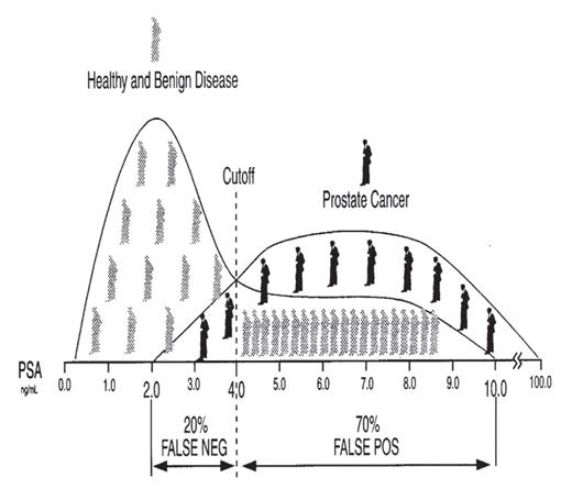
Dramatic representation of diagnostic sensitivity and specificity using the analyte prostate-specific antigen (PSA) as an example.
Visual inspection of Figure 2.2 reveals that, if the cutoff value, denoted by the dotted line at 4.0 ng/mL, is lowered to 2.0 ng/mL, the sensitivity of the PSA test improves from 80% at a cutoff of 4.0 ng/mL to 100% at a cutoff of 2.0 ng/mL since there are no false-negatives (ie, in this example, all individuals with prostate cancer have PSA values greater than 2.0 ng/mL). In addition, however, the number of false-positives increases, which causes the specificity of this test to worsen since specificity = TN/(TN + FP), because any increase in the number of false-positives, a term in the denominator of this equation, results in a decrease in the value given by this equation. Alternatively, if the cutoff value is increased to 10.0 ng/mL, the specificity of the PSA test improves from 30% at a cutoff of 4.0 ng/mL to 100% at a cutoff of 10.0 ng/mL since there are no false-positives (ie, in this example, all individuals without prostate cancer have PSA values less than 10.0 ng/mL). In addition, however, the number of false-negatives increases which causes the sensitivity of this test to worsen since sensitivity = TP/(TP + FN).
Lastly, it is important to remember that knowing the sensitivity (ie, positivity in disease) and specificity (ie, negativity in health or non-disease) of a test is of limited value because these parameters represent the answer to the question: What is the probability of a patient having a positive test result if this patient has disease X? The more challenging question facing clinicians, however, is: What is the probability of this patient having disease X if the test result is positive (or negative)?5 The reader is referred to reference 5 for a statistical briefing on how to estimate the probability of disease using likelihood ratios.
Receiver-Operator Characteristic (ROC) Curves
Receiver- (or relative-) operator characteristic (ROC) curves provide another useful tool in assessing the diagnostic accuracy of a laboratory test, because all (specificity, sensitivity) pairs for a test are plotted. The principal advantage of ROC curves is their ability to provide information on test performance at all decision thresholds.3,6
Typically, a ROC curve plots the false-positive rate (FPR = 1 - specificity) versus the true-positive rate (TPR = sensitivity). The clinical usefulness or practical value of the information provided by ROC curves in patient care may vary, however, even for tests that have good discriminating ability (ie, high sensitivity and specificity at a particular decision threshold). This may occur for several reasons:
False-negative results may be so costly that there is no cutoff value for the test that provides acceptable sensitivity and specificity.
The cost of the test and/or the technical difficulty in performing the test may be so high that its availability is limited.
Less invasive or less expensive tests may provide similar information.
The hardship (eg, financial and/or physical) associated with the test may cause patients to be unwilling to submit to the test.
A test with 100% sensitivity and 100% specificity in discriminating prostatic cancer from benign prostatic hyperplasia (BPH) and prostatitis at all decision thresholds would be represented by the y-axis and the line perpendicular to the y-axis at a sensitivity of 1.0 = 100% in a square plot of FPR versus TPR (Figure 2.3A).
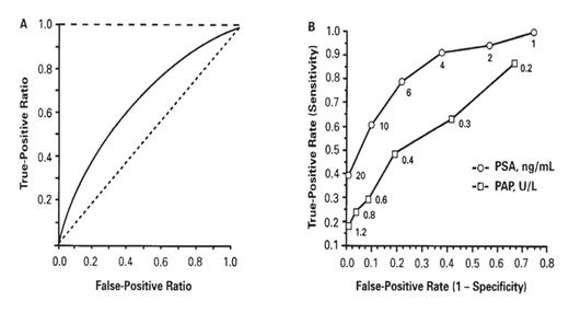
ROC curves for (A) perfect test (– – –), AUC=1.0; log prostate-specific antigen (PSA) concentration in discriminating organ-confined prostate cancer from benign prostatic hyperplasia (——), AUC=0.66 (95% confidence interval, 0.60–0.72); test with no clinical value (-----), AUC=0.50. (B) Prostatic acid phosphatase (PAP) and PSA in differentiating prostate cancer from benign prostatic hyperplasia and prostatitis at various cutoff values (indicated adjacent to points on each of the curves). Reproduced with permission from Nicoll CD, Jeffrey JG, Dreyer J. Clin Chem. 1993;39:2540–2541.
A test for which the specificity and sensitivity pairs sum to exactly 100% at all decision thresholds would be represented by the diagonal of the square (Figure 2.3A) and represents a test with no clinical value.
Thus, in qualitatively comparing 2 or more tests in their ability to discriminate between 2 alternative states of health using ROC curves, the test associated with the curve that is displaced further toward the upper left-hand corner of the ROC curve has better discriminating ability (ie, a cutoff value for the test can be chosen that yields higher sensitivity and/or specificity) than tests associated with curves that lie below this curve. A more precise quantitative estimate of the superiority of one test over another can be obtained by comparing the area-under-the-curve (AUC) for each test and applying statistics to determine the significance of the difference between AUC values.
The AUC (range: 0.5 to 1.0) is a quantitative representation of overall test accuracy, where values from 0.5 to 0.7 represent low accuracy, values from 0.7 to 0.9 represent tests that are useful for some purposes, and values >0.9 represent tests with high accuracy. The ROC curve (AUC = 0.66; 95% confidence interval: 0.60–0.72) in Figure 2.3A demonstrates that PSA has only modest ability in discriminating BPH from organ-confined prostate cancer.
However, other data using ROC curves to assess the ability of the tumor markers, prostatic acid phosphatase (PAP) and prostate specific antigen (PSA), to differentiate prostate cancer from BPH and prostatitis at various cutoff values is illustrated in Figure 2.3B. Qualitatively, the ROC curve corresponding to PSA is displaced further toward the upper left-hand corner of the box than the curve for PAP. Quantitatively, the AUC values for PSA and PAP are 0.86 and 0.67, respectively. Thus, both qualitative and quantitative ROC analysis demonstrates that PSA provides better discrimination than PAP in distinguishing men with prostate cancer from those with BPH or prostatitis. Moreover, the diagnostic accuracy (ie, sensitivity and specificity) of PSA in providing this discrimination is higher (AUC = 0.86) in Figure 2.3B than in Figure 2.3A (AUC = 0.66), probably due to differences in the study designs represented by the data shown in each panel of Figure 2.3.
Reference Interval for Interpreting Laboratory Test Results
Once a clinical laboratory test with the appropriate diagnostic accuracy has been ordered, how are the results of the test interpreted? Typically, a reference interval or a decision level is used, against which the patient’s test value is compared. Decision level refers to a particular cutoff value for an analyte or test that enables individuals with a disorder or disease to be distinguished from those without the disorder or disease. Moreover, if the diagnostic accuracy of the test and the prevalence of the disease in a reference population are known, then the predictive value of the decision level for the disorder or disease can be determined.
Reference interval relates to the values for an analyte (eg, PSA, glucose, etc.), determined on a defined population of “healthy” individuals, that lie between the lower and the upper limits that constitute 95% of all values. Thus, an analyte value less than the lower limit of the reference interval would be classified as abnormally low, while any value greater than the upper limit of the reference interval would be classified as abnormally high, and values in between these limits would be classified as “normal.” For example, after establishing the status of a population of individuals as “healthy,” using such methods as history, physical exam, and findings other than the test being evaluated, the reference interval for PSA, using many different assays, is typically stated as 0.0 ng/mL to 4.0 ng/mL. Thus, 95% of healthy men have a serum PSA concentration between these limits.
Although many laboratories publish the lower limit of a reference interval as “0,” no analytical assay is capable of measuring a concentration precisely equal to 0 with high reproducibility. All quantitative assays have a finite lower limit of detection (LLD), distinct from 0, that more precisely constitutes the lower limit of the reference interval when this lower limit encompasses 0. For many PSA assays, the LLD is typically 0.05 ng/mL. Therefore, any PSA value less than 0.05 ng/mL would be reported appropriately as “less than 0.05 ng/mL” and not as 0.0 ng/mL. In addition, it is important to remember that reference intervals for an analyte are method dependent (ie, the reference interval established using one method cannot automatically be substituted for that of a different assay that measures the same analyte).
Since reference intervals for all analytes are based typically on the limits for the analyte that include 95% of all values obtained on healthy individuals with the assumption that the distribution of these values is Gaussian (or “bell-shaped”), it is important to recognize that 5% (or 1 out of 20; ie, the 2.5% of healthy individuals with analyte values in the left tail of the data distribution and the 2.5% of healthy individuals with analyte values in the right tail of the distribution when the reference interval is defined as the limits of the 2.5th and 97.5th percentiles of the distribution of all analyte values obtained on healthy individuals) of healthy individuals will have values outside these limits, either low or high (Figure 2.4).
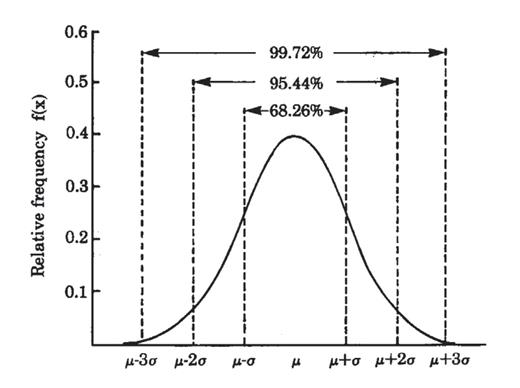
Example of a Gaussian (or bell-shaped) distribution of test values in which ~68% of the values are between the mean (μ) ± 1 standard deviation (σ); ~95% are between μ ± 2σ; and, ~99% are between μ ± 3σ.
Thus, reference intervals are intended to serve as a guideline for evaluating individual values and, for many analytes, information on the limits of an analyte for a population of individuals with the disease or diseases the test was designed to detect is even more informative. Also, it is important to recognize that values for some analytes in a population of healthy individuals may not be Gaussian distributed.
Figure 2.5 provides an illustration of this point applicable to the analyte, gamma-glutamyl transferase (GGT), in which the data is positively skewed. The reference interval for this data must be determined using a non-parametric statistical approach that does not make the assumption that the data is Gaussian distributed.
![Example of a distribution of laboratory test values for an analyte (ie, the liver enzyme, gamma-glutamyl transferase [GGT]) for which the data are not Gaussian distributed.](https://oup.silverchair-cdn.com/oup/backfile/Content_public/Journal/labmed/40/2/10.1309_LM4O4L0HHUTWWUDD/4/m_111fig2.5.jpeg?Expires=1716314019&Signature=l3zi4gLvSkGDkiu0ihrtFmfllpCNrItYuITbS208gYm0YXlBDA333XTq3rXtfVMT76KpfwX3eQOUSoGHR0i597sYx8QPyNM6SYpmUAieEJGxwx4uSE7c5i0EuSIPbTPIRw1uPR-Kbo1wXrDR9S0NerhTMM94BknN08IskgaAGE-qbxQfiI9bnfzjKZO81qrxPPePRbzdOxfe~I5EkLucKdyMYyDqTNeP7MoKEhwHcakL6IPx29RQRio8MEtR3751WhTGKin-86QLfm-hzImeeuaBZmAwHPGqdamvZcNP637qlu701W4CRFZGOCILd0OUJkihnxjF0d~wkBZ98Y0XRw__&Key-Pair-Id=APKAIE5G5CRDK6RD3PGA)
Example of a distribution of laboratory test values for an analyte (ie, the liver enzyme, gamma-glutamyl transferase [GGT]) for which the data are not Gaussian distributed.
Lastly, to accurately interpret test results, it may be necessary to know gender-specific and/or age-stratified reference intervals since the values for many analytes vary with developmental stage or age. For example, alkaline phosphatase, an enzyme produced by osteoblasts (bone-forming cells), would be expected to be higher in a healthy 10- to 12-year-old during puberty and the growth spurt (ie, increased bone formation during lengthening of the long bones) that normally accompanies puberty in adolescent males and females than those observed in a prepubertal or elderly individual.
Ideally, the best reference interval for an analyte would be individual-specific such that the value for the analyte, determined when the individual is ill, could be compared with the limits for this analyte, established on this same individual, when he or she was healthy or without the illness. For obvious reasons, it is difficult, if not impossible, to obtain such reference intervals. Thus, population-based reference intervals offer the most cost-effective and rational alternative. When using population-based reference intervals, however, it is critical that members of the reference population be free of any obvious or overt disease, especially diseases likely to affect the analyte for which the reference interval is being determined. For example, when determining a reference interval for TSH (also known as thyrotropin), it is critically important that the population of individuals tested be free of any pituitary or thyroid disease likely to affect the pituitary-hypothalamic-thyroid axis, which, under the action of the thyroid hormones tri- (T3) and tetraiodothyronine (T4), exert regulatory control over circulating levels of TSH.
Critical Difference Between Consecutive Laboratory Test Results
Since physicians frequently order the same test at multiple time points during the course of the patients’ management, they are faced with the challenge of interpreting when the magnitude of the change in values for an analyte constitutes a significant change (or critical difference [CD]) that may (or should) affect medical decision making (eg, trigger a change in therapy, such as increasing or decreasing a drug dosage). Quantitative values for all analytes are affected by both imprecision (ie, lack of reproducibility) in the measurement of the analyte and intra-individual variation over time in the concentration of the analyte due to normal physiologic mechanisms (ie, biological variation) that are independent of any disease process. For example, the analyte cortisol, a glucocorticoid produced by the adrenal cortex that is important in glucose homeostasis, normally displays diurnal variation. Blood cortisol levels begin to rise during the early morning hours, peak at mid-morning, and then decline throughout the day to their lowest level between 8 pm and midnight. In patients with Cushing’s syndrome, this diurnal variation is lost and blood cortisol levels remain elevated throughout the day.
The degree of imprecision (ie, lack of reproducibility) in the quantitative measurement of any analyte is given by the magnitude of the coefficient of variation (CV), expressed usually as a percent, obtained from multiple measurements of the analyte using the formula: %CV = (SD/mean) × 100; where mean and SD are the mean and standard deviation of the values obtained from the multiple measurements of an analyte. There is a direct relationship between the magnitude of the CV and the degree of imprecision (ie, the lower the CV, the lower the imprecision [or the higher the degree of precision]). The magnitude of analytical variation is given by CVa, while biological variability is defined by CVb. Approaches to determining assay-specific values for CVa, CVb, and CD are beyond the scope of this CE Update.
Fortunately, most assays for a wide variety of analytes have excellent precision (ie, <5% to 10% CVa), such that the principal component among these 2 sources of variation (ie, analytical or biological) is biological variation (CVb). In addition, a change in values for an analyte that exceeds the change (ie, reference change value [RCV]) expected due to the combined effects of analytical and biological variation alone is due most likely to a disease process or to the affect of any therapy on the disease.
Neural Networks
More recently, neural networks, a branch of artificial intelligence, have been used to evaluate and interpret laboratory data.7,8 These computerized networks mimic the processes performed by the human brain and can learn by example and generalize. Neural networks have been applied to such diverse areas as screening cervical smears (Pap smears) for the presence of abnormal cells and the identification of men at increased risk of prostate cancer by combining values for PSA, prostatic acid phosphatase (PAP), and total creatine kinase (CK). The use of neural networks in clinical and anatomic pathology is likely to expand because of their ability to achieve a higher level of accuracy than that attained by manual processes.
Laboratory Testing Paradox
Laboratory test results may influence up to 70 percent of medical decision making.9 However, one must wonder whether the test results are being interpreted correctly, and—if not—what the impact is of incorrect or inappropriate interpretation on the accuracy of diagnostic decision making based, in part, on laboratory test results. In a 2008 survey of junior physicians in the United Kingdom, only 18% of respondents were confident about requesting 12 common chemistry tests while more than half considered themselves usually confident or not confident in interpreting the results.10 The lack of confidence in interpreting laboratory test results may be directly related, as suggested by Dr. Lopasata, to the sparse training in laboratory medicine provided in most United States medical schools.
Conclusion
In the final analysis, it is important for clinicians and lab-oratorians to recognize that laboratory data, although potentially extremely useful in diagnostic decision making, should be used as an aid and adjunct to the constellation of findings (eg, history, physical exam, etc.) relevant to the patient. Laboratory data is never a substitute for a good physical exam and patient history (clinicians should treat the patient, not the laboratory results).
References
Author notes
After reading this paper, readers should be able to describe the “laboratory testing cycle” and discuss the potential sources of error that can occur in each phase of this cycle. Readers should also be able to describe the general principles for selecting the most appropriate laboratory test based on its diagnostic performance characteristics.
Chemistry 20903 questions and corresponding answer form are located after this CE Update article on page 114.
