Multiple Maxima of Likelihood in Phylogenetic Trees: An Analytic Approach

Abstract

Maximum likelihood (ML) is a widely used criterion for selecting optimal evolutionary trees. However, the nature of the likelihood surface for trees is still not sufficiently understood, especially with regard to the frequency of multiple optima. Here, we initiate an analytic study for identifying sequences that generate multiple optima. We concentrate on the problem of optimizing edge weights for a given tree or trees (as opposed to searching through the space of all trees). We report a new approach to computing ML directly, which we have used to find large families of sequences that have multiple optima, including sequences with a continuum of optimal points. Such data sets are best supported by different (two or more) phylogenies that vary significantly in their timings of evolutionary events. Some standard biological processes can lead to data with multiple optima, and consequently the field needs further investigation. Our results imply that hill-climbing techniques as currently implemented in various software packages cannot guarantee that one will find the global ML point, even if it is unique.

Introduction

Molecular data, and even complete genomes, are being sequenced at an increasing pace. This newly accumulated information should make it possible to resolve long-standing questions in evolution, such as reconstruction of the phylogenetic tree of placental mammals and estimation of the times of species divergence (Waddell, Okada, and Hasegawa 1999 ). The analysis of this data flood requires sophisticated mathematical tools and algorithmic techniques. The selection criteria of maximum likelihood (ML) is one of the most widely used and accepted in phylogeny. In general, the likelihood surface may be complex (Edwards 1972 ). We use analytic methods to investigate the likelihood surface for phylogenetic trees, and we demonstrate that it is indeed complicated. Even “biologically reasonable” sequence data can lead to a continuum of points, all attaining the same ML value.

ML on molecular sequence data uses a model of evolution, which is typically a family of trees with n taxa at their leaves, and a substitution model. The parameters of the substitution model describe probabilities of changes in character states (e.g., point mutations in DNA nucleotides). Given a set of n observed sequences, the goal is to find the best explanation for the data within the model space. In our context, this usually means a weighted tree (where the weights are parameters of the substitution model for each edge) which maximizes the likelihood (the conditional probability under the model of generating the observed sequences). There are two optimization problems related to ML in phylogenetics. The first is to optimize the branch (edge) lengths for a given tree or trees. The second is to find the ML tree by searching in the tree space. This paper deals with the first problem.

Previous Work

The current application of ML for reconstructing evolution is that of Felsenstein (1981) and has gained wide acceptance (Barry and Hartigan 1987 ; Goldman 1990 ; Saitou 1990 ; Swofford et al. 1996 ). The method is computationally intensive, but for tractable cases it is the method of choice. Algorithmically, the likelihood is maximized separately for each tree in the family (pruning is sometimes possible). The weighted tree (or trees) with maximum value(s) is then reported. There is no known analytical solution or direct algorithm that optimizes the edge parameters for a given tree (except for the simplest case of n = 3 taxa under a molecular clock, which was solved very recently by Yang [2000] ). Existing algorithms (Felsenstein 1995 ; Swofford 1998 ) use an iterative hill-climbing approach. For hill climbing to be guaranteed to find the maximum, there must be a single local and global maximum in the parameter space. Fukami and Tateno (1989) , and subsequently Tillier (1994) , have argued that for each tree, the ML point is indeed unique. However, Steel (1994) showed that their proof was erroneous and constructed a surprisingly simple counterexample (using sequences with just two sites and four taxa {1,2,3,4}).

Steel's (1994) work clearly demonstrates that caution should be exercised when ML solutions are sought. However, the two ML points of his counterexample require a substitution probability of p = 1/2 on two edges, so they represent points on the boundary of saturation for the underlying evolutionary model. Furthermore, these two ML points are on the tree T = (12)(34), which does not maximize the likelihood function across all trees. (The tree T = (13)(24) has a unique ML point that attains higher likelihood than each of the two ML points on T = (12)(34).) Steel recommended a numerical examination of more biologically reasonable data sets.

In their recent simulation study, Rogers and Swofford (1999) asked the question “Is it generally true that the trees of highest maximum likelihood for a given data set have only a single optimum?” They simulated data according to a variety of models. For each set of simulated data, they applied the numerical ML hill-climbing package of PAUP* (Swofford 1998 ) from 100 random starting points and recorded the number of distinct ML points reached. Although they did locate a small proportion of “true” (generating) trees that had more than one local maximum, in each case one of the ML points was the unique global optimum. They concluded that “the true tree rarely had multiple likelihood maxima.” Indeed, given the continuity of the likelihood function and the results of Goldman (1993) , Yang (1994) , and Rogers (1997) that the ML point is unique if the data fit a tree T exactly, it is probable that when the data are “close” to the exact fit on T, the ML point on T should be unique and global (see the Proofs section for further discussion on this point).

Our Work

In this paper, we seek to investigate this problem from a different perspective, to analytically study the likelihood surface for sequence data that is not necessarily “close” to a tree. Can we find data sets for which there are two (or many) global ML points? This will help us to gain a better understanding of the shape of the likelihood surface. The hope is that this approach would ultimately help in identifying cases in which there is a unique global and local ML point (so the traditional hill-climbing methods are adequate), as well as in identifying cases in which there is more than a single local maximum, such that alternative methods and models may be needed.

We take a first step in this direction by proving that multiple ML points do occur over a large range of sequence data. We employ Hadamard conjugation (Hendy and Penny 1993 ; Hendy, Penny, and Steel 1994 ), constrained optimization, and numerical methods in conjunction with symbolic mathematical software tools. We show that even for the simplest model of evolution (a symmetric Poisson model with 2-character states), with just four taxa, the best tree can have more than a single global ML point. For some special subfamilies, there are even continuous ML curves. Furthermore, these curves can intersect the parameter space in separate, disconnected components (so it is not possible to go continuously between some pairs of points along the ML curve).

The remainder of this paper is organized as follows: The Background and Definitions section contains background, definitions, and notations. In the Results and Discussion section, we describe our main results, illustrate them graphically, and discuss them. Proofs and relevant mathematical background are given in the Methods section. In the Hadamard Conjugate and the Likelihood Function section, we explain the Hadamard conjugate and derive a number of important lemma's that set up the framework for our analytic results. These results are rigorously proved in the Proofs section. Finally, the Conclusions section presents several implications of this work and points out some directions for further research.

Background and Definitions

In this section, we briefly describe the ML selection criteria as usually implemented in phylogenetic analysis. The goal of ML is to find the weighted evolutionary tree (or trees) which is most likely to have produced the observed sequence data. To make this notion meaningful, we must have an underlying substitution model for the process of point mutation. Then, we seek the tree(s) T, together with the edge probabilities p_e (or weights) which maximize L, the likelihood of the data. The ML criterion is usually applied to 4-state (DNA and RNA nucleotide) or 20-state (protein amino acid) sequences. However, much understanding can be gained by applying the criteria to the simpler case of just 2-state characters, x and y.

Notation 1. We denote by n the number of species (or taxa), and by c the length of the observed sequences. We use boldface to denote vectors (e.g., P, q, s, 0). The edge set of a tree T is denoted by E(T). Summations over subsets, like Σ_δ, are over all subsets δ of {1, … , n − 1}, except in cases that explicitly indicate a different range.

Our analysis uses the symmetric Poisson model, where for each edge e of a tree T, we have a corresponding probability p_e (≤1/2) that the character states at the two incident vertices of e differ, and this probability is independent of the state at the initial vertex (the Neyman (1971) two-state model). In this symmetric case, it is readily seen that p_e is independent of the position of the root, so in our analysis we will regard the trees T as unrooted.

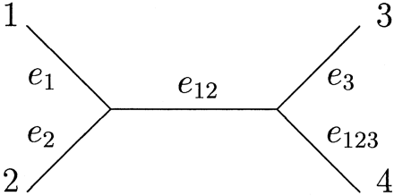
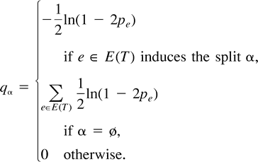
We now introduce a notation that we will use for labeling the edges of unrooted binary trees. This notation greatly simplifies the use of the Hadamard conjugate (see Hadamard Conjugate and the Likelihood Function), which is a central tool in our analysis. (For simplicity, we use four taxa, but the definitions extend to any n.) Suppose the four species, 1,2,3, and 4, are represented by the leaves of the tree T′. A split of the species is any partition of {1,2,3,4} into two disjoint subsets. We will identify each split by the subset which does not contain 4 (in general, n), so that, for example, the split {{1,2}, {3,4}} is identified by the subset {1,2}. Each edge e of T induces a split of the taxa, namely, the two sets of leaves on the two components of T resulting from the deletion of e. Hence, the central edge of the tree T′ = (12)(34) in the brackets notation induces the split identified by the subset {1,2}. For brevity, we will label this edge e₁₂, as shorthand for e_{1,2}. Thus, E(T′) = {e₁, e₂, e₁₂, e₃, e₁₂₃} (see fig. 1 ).

For a tree T, let p = [p_e]_e∈E(T) be the edge probabilities. Let ψ = [ψ(1), ψ(2), ψ(3), … , ψ(c)] ∈ {x, y}^{n × c} be the observed sequences of length c over n taxa. The likelihood of observing ψ, given the tree T and the edge probabilities p, L(ψ | T, p) has the form

where a ranges over all combinations of assigning characters states (x or y) to the n − 2 internal nodes of T. This notion of ML is termed the maximum average average likelihood in Steel and Penny (2000) . Each m( p_e, ψ_i, a_i) is either p_e or (1 − p_e), depending on whether in the ith site of ψ and a the two endpoints of e are assigned different character states (m( p_e, ψ_i, a_i) = p_e) or the same character states (m( p_e, ψ_i, a_i) = 1 − p_e). See Felsenstein (1981) , Steel (1994) , and Tuffley and Steel (1997) for details.

The ML solution(s) for a specific tree T is the point (or points) in the edge space p = [p_e]_e∈E(T) (where 0 ≤ p_e ≤ 1/2) that maximizes the expression L(ψ | T,p). The global ML solution(s) is the pair (or pairs) (T,p) maximizing the likelihood over all trees T of n leaves and all edge probabilities p.

It is not hard to see that interchanging any two columns of ψ does not change the likelihood in equation (1) . It is thus convenient to “summarize” the observed data ψ by its observed sequence spectrum, ŝ. This spectrum simply counts how many sites share any specific pattern. Under a fully symmetric model, the probability of a pattern is equal to that of its complement (where all x and y are interchanged). We make the same conventions about indexing the patterns obtained in the sequences as we did for labeling the edges of a tree T. For example, consider the case n = 4 with species labeled 1, 2, 3, and 4. We identify a site pattern by the subset of species {1, 2, 3} whose character at that site is different from that of species 4. In general, for every α ⊆ {1, … , n − 1}, an α-split pattern is a pattern where all taxa in the subset α have one character (x or y), and the taxa in the complement subset have the second character (there are two such patterns). The value ŝ_α equals the number of times that α-split patterns appear in the data. If n = 4, then there are 2³ = 8 possible patterns, indexed by the subsets of {1, 2, 3}, and ŝ = [ŝ₀, ŝ₁, ŝ₂, ŝ₁₂, ŝ₃, ŝ₁₃, ŝ₂₃, ŝ₁₂₃] (e.g., ŝ₀ counts the constant patterns

while

are counted by ŝ₁₃).

Given a tree T with n leaves and edge probabilities p = [ p_e]_e∈E(T) (0 ≤ p_e ≤ 1/2), the probability of generating an α-split pattern (α ⊆ {1, … , n − 1}) is well defined (and equal for all sites). Denote this probability by ŝ_α = Pγ(α − split | T,p). Using the same indexing scheme as above, we define the expected sequence spectrum s = [s_α]_{α⊆{1, … ,n − 1}}. Having this spectrum at hand greatly facilitates the calculation and analysis of the likelihood, since the likelihood of observing ŝ given s is

Definition 1. Let T be a tree with n leaves. The edge length spectrum q = [q_α]_{α⊆{1, … ,n − 1}} of T is the following 2^{n − 1} dimensional vector:

In the two-state model, p_e is the probability of having an odd (1, 3, 5, …) number of substitutions per site across the edge e. If the underlying substitution model is a symmetric Poisson process, then q_e has a natural meaning as the expected number of substitutions per site across e equals q_e = −1/2 ln(1 − 2p_e). Measuring the edges by q_e, we get an additive measure on the tree (since expected values are additive). When drawing weighted trees, we usually refer to q_e as the length of the edge e. Elsewhere, we refer to q_e as the weight of the edge e. If for some e∈E(T), p_e = 0.5, then q_e is ill defined (+∞). This motivates us to restrict ourselves to the realistic cases where p_e < 0.5 (so q_e is finite) for all edges e of T.

Results and Discussion

Here, we describe several families of sequence data for which the best ML tree has multiple ML solutions. For simplicity, all our examples have just four taxa, and most of them have rather short sequences. However, the same phenomena are easily generalized to larger numbers of taxa and to longer sequences.

Main Results

Theorem 1.The following three observed sequence spectra yield a continuum of ML points on the tree (12)(34):

All three of these data sets have closed-form ML solutions. Furthermore, the ML points for data set (B) consist of two disconnected regions of edge weights on the tree (12)(34).

Table 1 illustrates the sequence data for these three data sets.

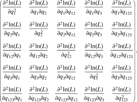
The proof of Theorem 1 is given in the proofs section. The essence of the proof is to represent the set of ML points in terms of the first-order partial derivatives of the log likelihood function. This gives rise to systems of polynomial equations (one per data set), which we then solve. Because these systems are fairly complex (nine polynomial equations of degree 4 in nine variables), we used the symbolic manipulation package MAPLE to obtain closed-form solutions. Finally, to verify that the solutions were indeed maximum points of the likelihood function, we checked that the second-order partial derivatives (the eigenvalues of the Hessian) were all nonpositive.

We now describe the ML solutions in detail, starting with data set (A). The symmetries in this data set imply that the multiple ML points occur not only on the tree (12)(34), but on each of the two other trees, (13)(24) and (14)(23), as well. The three trees (12)(34), (13)(24), and (14)(23) will exhibit the same ML values and nature of solutions. (Of course, the symmetries by themselves do not imply multiple ML points for each tree). For the tree (12)(34), the ML points form two families of solutions, which we denoted by sol_I and sol_II. Each family can be described as a one-dimensional line segment (parametrized by z, − 3 ≤ z ≤ 3), a “ridge” in the eight-dimensional parameter space described below:

These two ridges intersect at a single point (z = 0 in both curves).

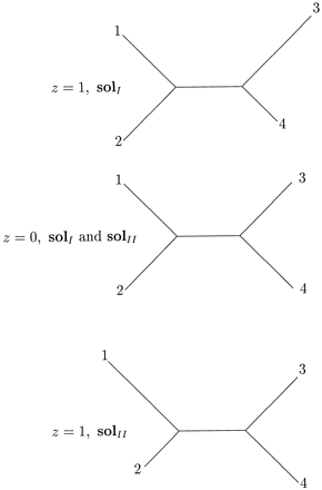
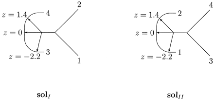
Figure 3 illustrates the three weighted trees corresponding to z = 1 and to z = 0 on the curves sol_I and sol_II of equation (3) . (For z = 0, the two curves yield exactly the same tree.) These three optimal trees represent rather different evolutionary histories. Figure 4 gives a graphical depiction of the two families of weighted trees, sol_I and sol_II, that maximize the likelihood for the observed sequence spectrum ŝ= [7, 0, 0, 1, 0, 1, 1, 0] as a function of the parameter z on the tree (12)(34). The family of trees on the left corresponds to sol_I, while the right side corresponds to sol_II. For sol_I, the lengths q₁ and q₂ both equal 1/4 ln (5/3) ≈ 0.127 (the same lengths, regardless of z). The length q₁₂ equals 1/2 ln 15 − 1/4 ln [(12 + z)(12 − z)]. It varies only slightly, with minimum value 0.111 at z = 0 and maximum value 0.127 for z = ±3. The length q₃ equals 1/4 ln[5(12 + z)/3(12 − z)], varying from 0 for z = −3 to 0.255 for z = 3. The lengths of the paths q₃ + q₁₂₃ equal the constant 1/2 ln(5/3) ≈ 0.255. For z < −3, the length q₃ would be negative, while for z > 3, the length q₁₂₃ would be negative. The curve sol_II exhibits a similar behavior, where the roles of q₁, q₂ and q₃, q₁₂₃ are interchanged, respectively.

The dependency of the edge lengths as a function of z forced us to use a non-conventional way of drawing these families of trees, in an attempt to produce a figure in which the lengths were approximately to scale. In particular, the edge length q₁₂ changes only slightly, while q₃ and q₁₂₃ vary substantially (keeping their sum invariant), so we put leaves 3 and 4 on the ends of a semicircular arc. The edge q₁₂ starts as a fixed line segment along the horizontal axis. It then makes a turn, continuing along a second line segment toward the arc. The angle between these two segments varies continuously with z. for z = −3, the variable part points exactly at one end of the arc, making the length q₃ equal 0. For z = 3, the variable part points exactly at the other end of the are, making the length q₁₂₃ equal 0. The “axis point” where q₁₂ makes a turn is slightly to the left of the semicircle's center. This way, the length q₁₂ increases slightly as z goes from 0 to ±3. The trees for z = −2.2, 0, 1.4 appear explicitly in the figure for both families. (The scale in Fig. 4 is slightly different than that in Fig. 3 .)

Example (B) is not symmetric, and the ML tree is (12)(34). The ML set is the intersection of the curve

with the two regions −33 ≤ z ≤ −17 and 17 ≤ z ≤ 33. Therefore, the ML points of data set (B) form two disconnected components.

Figure 5 illustrates the two weighted trees corresponding to z = −25 and to z = 25 on the curve sol_B of equation (4) . Again, these two optimal trees represent different evolutionary histories. Figure 6 gives a graphical depiction of the whole family of weighted trees sol_B that maximize the likelihood for the observed sequence spectrum ŝ = [14, 0, 0, 3, 0, 2, 1, 0] as a function of the parameter z. The family of trees on the left corresponds to values of z in the interval [−33, −17], while the right side corresponds to values of z in the interval [17, 33]. For each such z, the corresponding tree is obtained from figure 4 by drawing a line from the point corresponding to z on the 1 − 2 path, through the midpoint, to the 3 - 4 path. The trees for |z| = 17, 25, 33 appear explicitly in the figure. The length q₁ = 1/4 ln[10(187 + z)/(7(187 − z))]. The length q₃ equals 1/4 ln[10(z + 3)/(u(z − 3))]. The lengths of the two paths q₁ + q₂ and q₃ + q₁₂₃ equal the same constant 1/2 ln(10/7). The edge length q₁₂ equals 1/4 ln[(280z)²/(187² − z²) (z² − 3²). The two separate regions of ML trees are clearly demonstrated in figure 4 . All lengths are to scale (slightly different than in figure 5 ). For |z| outside the interval [17, 33] one of the four lengths q₁, q₂, q₃, and q₁₂₃ is negative.

Example (C) is not symmetric either and the ML tree is (12)(34). Here, the ML points lie on the simpler, one-component curve

where the parameter z varies in the range 4 ≤ z ≤ 10.

Because of the complexity of the systems of polynomial equations, we needed MAPLE (or a similar symbolic manipulation system) for solving them. However, it is much simpler to verify that the different solutions produced by MAPLE indeed satisfy the different conditions by employing simpler software like EXCEL and substituting our curves into the appropriate equations, using the different identities that we state and prove in the Methods section. (In general, it is easier to verify a proof than to come up with one.) The only point which may shed some doubt on the proof is the possibility that MAPLE may have missed some additional solutions. Even if this is the case, the curves we found still represent local maximum points. Furthermore, we used hill climbing from many different random starting points and always converged to points on the specified curves. This implies that even if additional local maxima do exist, their zones of attraction are extremely small.

Additional data sets

The three specific examples (A), (B), and (C) in Theorem 1 are not the only data sets with a continuum of ML solutions. These three examples are just representatives of larger families, having ML solutions of a similar nature. It is possible to obtain closed-form expressions for the general classes in Theorem 1, but these expressions are cumbersome. These general expressions are quite hopeless when it comes to the eigenvalues of the Hessian whose analysis is required in the proof. Therefore, we chose to analyze in detail just three specific examples that represent the general cases well.

To demonstrate the wide occurrence of data sets with continuum ML points, we further studied the following 74 cases. In all of them, closed-form solutions are obtainable, and each of these data sets gives rise to a continuum of ML solutions:

1. ŝ = [6 + i, 0, 0, 1, 0, 1, 1, 0] (1 ≤ i ≤ 20) — all 20 of these data sets have ML solutions with properties similar to those of (A).

2. ŝ = [14 + 8i + 4j + k, 0, 0, 3 + 2i + j, 0, 2 + i, 1, 0] (0 ≤ i, j, k ≤ 2) — all 27 of these data sets have ML solutions with properties similar to those of (B).

3. ŝ = [10 + 3i + 2j + k, 2 + i, 2 + i, 4 + i + j, 0, 1, 1, 0] (0 ≤ i, j ≤ 2, 1 ≤ k ≤ 3) — all 27 of these data sets have ML solutions with properties similar to those of (C).

All of the singleton entries (ŝ₁, ŝ₂, ŝ₃, ŝ₁₂₃) in the observed sequence spectra for data sets (A) and (B) of Theorem 1 are 0. This means that changes in the corresponding entries of the expected sequence spectra (ŝ₁, ŝ₂, ŝ₃, ŝ₁₂₃) do not affect the likelihood (of course, the resulting s must still fit a tree). In data set (C) the singleton entries ŝ₃ and ŝ₁₂₃ are both zero, so changes in ŝ₃ and ŝ₁₂₃ do not affect the likelihood. Initially, such examples were chosen because having some zero entries in ŝ makes it easier to find the analytic solution. We now show examples with multiple ML points in which all eight entries are nonzero.

Theorem 2. There are instances in which all eight entries in the observed sequence spectrumŝ = [ŝ₀, ŝ₁, ŝ₂, ŝ₁₂, ŝ₃, ŝ₁₃, ŝ₂₃, ŝ₁₂₃) are nonzero, yet the likelihood function has multiple maxima (two ML points).

Proof. The basic idea is to start from data sets like the one in example (B) with two separate regions of ML trees, and then make small changes to the singleton entries so that they are all positive. Since the likelihood function is “well behaved,” continuity arguments guarantee that for small enough perturbation, the two ML regions will remain separate. A small perturbation may turn a continuous ML curve into a single ML point, but these points will still remain separated, so we should get at least two separate maxima points.

We verified this intuition by using numerical methods. For example, the observed sequence spectrum

\[\mathbf{{\hat{s}}}\ {=}\ {[}1400,\ 1,\ 1,\ 300,\ 1,\ 200,\ 100,\ 1{]}\]

is a small perturbation of

\[\mathbf{{\hat{s}}}\ {=}\ {[}1400,\ 0,\ 0,\ 300,\ 0,\ 200,\ 100,\ 0{]}.\]

The latter is nothing but data set (B) (with ŝ = [14, 0, 0, 3, 0, 2, 1, 0]) in disguise, as multiplying all entries of an observed sequence spectrum by a constant (100 in this case) does not change the likelihood surface. Using numerical hill climbing with many random starting points, we verified that ŝ = [1400, 1, 1, 300, 1, 200, 100, 1] does indeed give rise to two separate ML points on the tree (12)(34). (The likelihood on the other two trees attains smaller maximal values.) Within the memory and time resources of our machine we could not find these two ML solutions analytically.

Table 2 demonstrates three more examples of the same nature. We remark that for all these examples, the likelihood is maximized on the tree (12)(34) (and, in some of these, on one or both of the other two trees as well).

In particular, the last example has a unique point a, which is a global maximum on (12)(34), and a unique point b, which is a local maximum on (12)(34). It also has a unique point c, which is a global maximum on (13)(24), and a unique point d, which is a local maximum on (13)(24). The value of the likelihood function L at point c is larger than its value at point b, so we have L(a) > L(c) > L(b) > L(d). □

Finally, we note that our results for n = 4 taxa could be generalized to yield trees on n taxa (leaves) with 2^n/4 ML regions. One way to achieve this is to grow a complete binary tree. At each level, we join two identical subtrees while making the coefficient of that split in ŝ large enough so that the two subtrees behave “sufficiently independently.” At the bottom level (trees on four leaves), we plant any instance of our multiple ML trees. Tuffley and Steel (1997) used a different technique to generalize Steel's (1994) multiple ML example from 4 to n species (with exponentially many ML points).

Methods

In this section, we give a complete proof of Theorem 1. Readers who are not interested in these mathematical details may skip directly to the Conclusions section, which contains conclusions and open problems. The Hadamard conjugate plays a crucial role in several key points of the proof. In the next section, we explain this transformation in detail and derive a number of new identities for the partial derivatives of the log likelihood function. These identities are later used in the Proofs section.

Hadamard Conjugate and the Likelihood Function

The Hadamard conjugation (Hendy and Penny 1993 ; Hendy, Penny, and Steel 1994 ) is an invertible transformation linking the probabilities of site substitutions on edges of an evolutionary tree T to the probabilities of obtaining each possible combination of characters. It is applicable to a number of simple models of site substitution: The Neyman (1971) 2-state model, the Jukes-Cantor model (Jukes and Cantor 1969 ), and the Kimura (1983) 2ST and 3ST models. For these models, the transformation yields a powerful tool which greatly simplifies and unifies the analysis of phylogenetic data. In this section, we explain the Hadamard transform and prove a number of technical lemmas expressing the partial derivatives of the likelihood function. These expressions are crucial in our approach to identify and analyze the points at which the likelihood function is maximized.

Definition 2. A Hadamard matrix of order l is an l × l matrix A with ±1 entries such that A^tA = lI_l.

We will use a special family of Hadamard matrices, called Sylvester matrices in MacWilliams and Sloane (1977 , p. 45), defined inductively for n ≥ 0

It is convenient to index the rows and columns of H_n by lexicographically ordered subsets of {1, … , n}. Denote by h_αγ the (α, γ) entry of H_n, then h_αγ = (−1)^|α∩γ|. This implies that H_n is symmetric, namely H_n^t = H_n, and thus by the definition of Hadamard matrices H_n⁻¹ = 2⁻H_n.

Proposition 1 (Hendy and Penny 1993 ). If p < 1/2 thens = s(q) =H⁻¹ exp (Hq), where H = H_n−1, namely, for α ⊆ {1, … , n − 1}, s_α = 2⁻⁽ⁿ⁻¹⁾ Σ_γh_αγ (exp (Σ_δh_γδq_γ). Furthermore, the transformation is reversible, so if Hs > 0, thenq = q(s) = H⁻¹ ln (Hs).

We call this transformation the Hadamard conjugate. For n taxa, the time complexity of computing it is O (n2ⁿ), and the space complexity is O (2ⁿ) (using the FFT-like fast Hadamard multiplication; Hendy and Penny 1993 ; Hendy, Penny, and Steel 1994 ). This “low exponential” complexity makes it applicable in cases with n of up to 30 taxa (usually this is not the bottleneck in phylogenetic analysis of moderate-sized trees for this model).

Spectral analysis makes it possible to compactly express the partial derivatives of the likelihood function. This, in turn, helps in identifying points at which the likelihood is maximized. We now present a number of new results along these lines. These results are of a technical nature, but they are important for the later derivations, as well as in additional contexts. Let α·β denote the symmetric difference of the two subsets α and β (α, β ⊆ {1, … , n − 1}).

The following lemma specifies the rate of change in any component s_α (the expected sequence spectrum) with respect to the rate of change in any component q_β (the expected number of substitutions along an edge in the underlying phylogenetic network). It proves that this partial derivative is simply the difference s_α·β − s_α. Being able to express the partial derivative directly is a major advantage. Notice that α may equal β in this lemma.

Lemma 1. Letqbe an edge length spectrum, and letsbe the corresponding expected sequence spectrums = s(q) = H⁻¹ exp (Hq). Then, the partial derivative of s_α, the α component ofswith respect to q_β, the β component ofq (α, β ⊆ {1, … , n − 1}, β ≠ ø) equals

Proof.

By Proposition 1,

so we have

(the relation q_ø = −Σ_δ≠øq_δ is used in (*), while (**) use the identity h_αγh_γβ = h_(α·β)γ).□

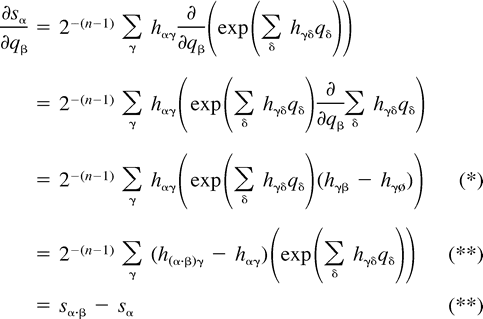
The next two lemmas describe the rate of change of the log likelihood function with respect to changes in the edge parameter q_β (Lemma 2) or the expected sequence parameter s_β (Lemma 3). These two lemmas are heavily used later to analyze the ML points. The proof of Lemma 2 makes repeated use of Lemma 1. Recall that α·β denotes the symmetric difference of the two subsets α and β.

Lemma 2. The partial derivative of the log likelihood function ln L(ŝ | s) with respect to the edge parameterq_βcan be expressed in terms of the observed and expected sequence parameters as follows for splits β that correspond to an edge of T,

The second-order partial derivatives for splits β_1, β₂that correspond to an edge of T are

Proof. By equation (2) , ln L(ŝ | s) = Σ_ŝα>0ŝ_α ln(s_α), so

Taking a second derivative and applying Lemma 1 again, we get

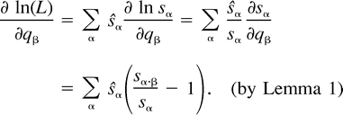
Using the relation s_ø = 1 − Σ_α≠øs_α and formulation (2) of the likelihood function, we get:

Lemma 3. The partial derivatives of ln(L) with respect tos_β (for any nonempty subset β of {1, … , n − 1}) equal

and the second-order partial derivatives are

Proof. The proof is a standard application of the multinomial distribution. We omit the details.

Before searching for data sets with multiple ML points, it is necessary to make some definitions. The following definition of “conservative data” aims at excluding data sets that are pathological, are biologically unrealistic, and could lead to negative edge weights on the tree.

Definition 3. Let ψ = [ψ(1), ψ(2), ψ(3), … , ψ(c)] ∈ {x, y}^n×c be the observed sequences of length c over n taxa, and let ŝ be the observed sequence spectrum. We say that ŝ is conservative if Hŝ > 0.

For the observed sequence spectrum in Steel's (1994) paper, ŝ = [0, 0, 0, 0, 0, 2, 0, 0], we have Hŝ = [2, −2, 2, −2, −2, 2, −2, 2], so ŝ is not conservative. If the number of constant sites, ŝ_ø, is greater than the sum of all other sites, namely, ŝ_ø > Σ_α≠øŝ_α, then ŝ is conservative. However, this sufficient condition is not necessary. Data sets (A), with ŝ = [7, 0, 0, 1, 0, 1, 1, 0], and (B), with ŝ = [14, 0, 0, 3, 0, 2, 1, 0], satisfy the condition. Data set (C), with ŝ = [10, 2, 2, 4, 0, 1, 1, 0], does not satisfy this condition, as ŝ_ø = Σ_α≠øŝ_α. However, Hŝ = [20, 6, 6, 8, 16, 6, 6, 12], so this observed sequence spectrum is indeed conservative too.

Definition 4. Let ŝ be the observed spectrum of ψ ∈ {x, y}ⁿ. If ŝ is conservative, then its conjugate spectrum is the vector q̂ = H⁻¹ ln(H(1/cŝ)).

If ŝ perfectly matches the expected sequence spectrum ŝ (namely, ŝ = cs), then the conjugate spectrum q̂ equals the edge length spectrum q, but in reality, ŝ is a finite sample of cs, and a perfect match is not expected. This implies that usually most of the entries of the conjugate spectrum q̂ are nonzero, and frequently some are negative. Even if q̂ does not represent a tree, it is still a useful representation which may be applied in searching for a plausible tree that has generated the data (see the closest-tree algorithm of Hendy [1991] ). This motivates us to define the splits space, which is the collection of all possible edge length spectra q.

Definition 5. The (order n) splits space is the subset of the 2ⁿ⁻¹-dimensional real vector space containing all vectors whose components sum to 0

Figure 2 illustrates the order n splits space for n = 4. An α-split corresponds to the collection of parallel edges that separate the subset of nodes α ⊆ {1, … , n − 1} from its complement {1, … , n}\α. (These parallel edges are all of the same length q_α.) We note that for n ≥ 4, the set of tree spectra q(T) over all weighted trees T with n leaves is a proper subset of the positive quadrant (set of vectors q with nonnegative entries) of the order n splits space.

Proofs

Before the proof of Theorem 1, we quote two known results regarding ML over the splits space. These results state that in the splits space, there is always a unique ML point. Furthermore, if the observed data exactly fit a weighted tree, then this weighted tree is the unique optimum.

Proposition 2 (Goldman 1993 ; Yang 1994 ). Ifŝis conservative, then the (unconstrained) likelihood functionL(s | ŝ) has a unique maximum over the splits space at the points = 1/cŝ.

The next proposition is by Rogers (1997) , where it is stated and proved for the general model of reversible substitutions. In this model, the probabilities of observing a change after t units of time from character state i to character state j and from j to i are the same. We present an alternative, simpler proof. However, our proof is valid only for the substitution models for which the Hadamard transform is applicable. This class of models is narrower than the class of general reversible models.

Proposition 3. Suppose the observed spectrumq̂fits exactly the expected edge spectrumq = q(T) for a weighted tree T with nonsaturated edge weights 0 ≤ P < 1/2. Then, T is the (unique), ML tree, with each edge e_αof T having weightq_α.

Proof. By Proposition 1, the expected sequence spectrum q satisfies the equality q(T) = q = H⁻¹ln(Hs). By definition, the conjugate spectrum q̂ is the vector q̂ = H⁻¹ln(H(1/cŝ)). Since q = q̂ by assumption, we have H⁻¹ln(Hs) = H⁻¹ln(H(1/cŝ)). Multiplying on the left by H, we get ln(Hs) = ln(H(1/cŝ)). Exponentiating each entry, we have Hs = H(1/cŝ). Since H is an invertible matrix, this last equality implies s = 1/cŝ.

Now suppose, by way of contradiction, that q′ = q′(T′) for another weighted tree T′ (q′ ≠ q), and s′ = H⁻¹exp(Hq′). Since the transformation is one-to-one, s ≠ s′. By Proposition 2, L(s′ | ŝ) < L(s | ŝ), namely, the likelihood of the data for T′ is smaller than the likelihood for T. Therefore T is the ML tree, and every other weighted tree T′ attains a smaller likelihood.

We remark that essentially the same proof applies to 4-state nucleotides under those substitution models where the Hadamard transform is applicable. A comprehensive work discussing more general Markov models on evolutionary trees can be found in Chang (1996) . Chang proves that under fairly mild conditions, the ML method is consistent for reconstructing the underlying evolutionary tree.

Since the likelihood function is continuous, continuity arguments imply that for edge spectra that are “close” to one that fits a tree exactly, we would expect a “nearby” weighted tree to be the single ML point. We make it clear that this argument, as well as the rest of our paper, does not deal with the effect of model complexity on the existence of multiple optima. We assume an underlying model, like the Neyman (1971) 2-state model. Within that model, we distinguish between data that are very “treelike” and data that are not “treelike.”

Another observation is that for n = 3 there is a single (unweighted) tree, and in this case the tree spectra and the nonnegative quadrant of the splits space coincide. This means that if we seek data sets giving rise to multiple ML points, then n must be at least 4. Combining both observations, we look for data sets on n = 4 taxa that do not fit a tree closely. By following this intuition, we arrived at data sets (A), (B), and (C) of Theorem 1. We now proceed to the proof of that theorem. In particular, we show that these three data sets give rise to a continuum of ML points.

Proof of Theorem 1. Out data sets (A), (B), and (C) have observed sequence spectra of the form ŝ = [ŝ_ø, ŝ₁, ŝ₂, ŝ₁₂, 0, ŝ₁₃, ŝ₂₃, 0]. By equation (2) , such observed sequence spectra give rise to the following expression for the log likelihood function:

(For data sets (A) and (B), the two terms ŝ₁lnŝ₁ + ŝ₂lnŝ₂ vanish, since the corresponding coefficients ŝ₁ and ŝ₂ are 0.)

Our goal is to maximize ln(L) over the 8-dimensional space s = [s_ø, s₁, s₂, s₁₂, s₃, s₁₃, s₂₃, s₁₂₃], bound to the constraint that s represents a point in the probability space of a tree T (i.e., the corresponding edge spectrum q = H⁻¹ln(Hs) represents T). The constraints on s are the eight inequalities 0 ≤ s_α ≤ 1 and the equality s_ø = 1 − Σ_α≠øs_α. Furthermore, s represents a point on the probability set of a tree if

1. q_α ≥ 0 for all α ∈ E(T ).

2. q_α = 0 for all α ∉ E(T ) ∪ {ø}.

Thus, for the tree T = (12)(34), q₁₃ = q₂₃ = 0; for T = (13)(24), q₁₂ = q₂₃ = 0; and for T = (14)(23), q₁₂ = q₁₃ = 0.

In order to solve the constrained optimization problem for the tree, we first express the two constraints q₁₃ = 0 and q₂₃ = 0 in terms of the eight components of s, using the relation s = s(q) = H⁻¹exp(Hq). (This is the first place at which the Hadamard conjugate plays a crucial role in the proof.) As the expressions of q₁₃ and q₂₃ involve logarithms and are somewhat cumbersome, we apply further simplifications to these two equations, leading to

We denote these last two equations by f = 0 and g = 0. (Constraints of a similar nature were derived by Cavender and Felsenstein [1987] .) Using the fact that the sum of the eight components in s is 1, we eliminate the variable s_ø.

We now use Lagrange multipliers to find the turning points of ln L, bound by the two constraints f = 0 and g = 0. (After the solution is found, we must check that the turning points satisfy 0 ≤ p_e < ½ (or, equivalently 0 ≤ q_e < ∞) for each edge e ∈ E(T ).) For each of the seven nonempty subsets α ⊆ {1, 2, 3}, we have the equation

Together with the two constraints, we get a system of nine equations in nine variables—the seven s_α variables and the two Lagrange multipliers μ and λ. This system of degree 4 polynomial equations is too involved to solve manually, so we applied the Maple V mathematical package. The nature's of the solutions differ according to the equality/inequality relations among the values ŝ₁₂, ŝ₁₃, ŝ₂₃, ŝ₁, ŝ₂. (Alternatively, we could use a system of equations stemming from the partial derivatives with respect to q_β [eq. (6)] . Despite its more elegant appearance, the resulting system has proved less tractable than the one we use.)

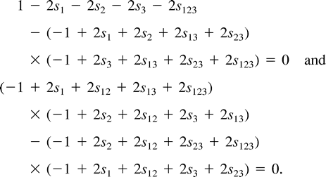
The symmetries in example A imply that the three trees (12)(34), (13)(24), and (14)(23) will exhibit the same ML values and nature of solutions. (Of course, the symmetries by themselves do not imply ML points for each tree.) For the tree (12)(34), the turning points form two families of solutions, denoted by sol_I and sol_II. Each family can be described as a one-dimensional line segment (parameterized by z, −4 ≤ z ≤ 4), a “ridge” in the eight-dimensional parameter space described in equation. (3). These two ridges intersect at a single point (z= 0 in both curves). Combining the constraints that all the edges in the tree have nonnegative weights (q₁, q₂, q₁₂, q₃, q₁₂₃≥ 0), each ridge is further restricted to the subinterval −3 ≤ z ≤ 3.

It remains to verify that sol_I and sol_II are indeed maxima of L. For this proof, it is more convenient to switch back to the “q-representation” (partial derivatives with respect to the q_β variables). We compute the 5-by-5 Hessian of the log likelihood ln L with respect to q₁, q₂, q₁₂, q₃, q₁₂₃:

We express the second-order partial derivatives in terms of the s_α values using equation (7) and then substitute the values of sol_I curve (eq. (3) ). (This is the second place at which the Hadamard conjugate plays a crucial role in the proof). A turning point is a (local) maximum if no eigenvalue of the Hessian is positive and at least one eigenvalue is negative. (The Hessian is a real symmetric matrix, so all at its eigenvalues are real). In our case, the characteristic polynomial has five real roots (the five eigenvalues). With MAPLE's help, we found that the characteristic polynomial over the ridge sol_I (a polynomial of degree five in the formal variable t) is

It has three linear factors, giving rise to the nonpositive roots t = 0, t = −45 and t = −4z² (One of the eigenvalues equals 0, since there is one direction on this ridge where the value of L is unchanged. When z = 0, the two ridges intersect and there are two directions where L is unchanged). Factoring out these three linear terms, we are left with the degree 2 polynomial (7t² + 621t + 12,920 + tz² + 45z²)/7. Clearly, the value of this last polynomial is strictly positive for any nonnegative value of t. Therefore, its two roots must be negative. As an additional verification step, we also applied an iterative hill-climbing algorithm with many starting points to the function in L. As expected, the only maxima points detected were along the two ridges sol_I and sol_II.

Example B is not symmetric, and the most parsimonious tree for these data is (12)(34), inducing a total of nine changes. This indicates (but, of course, does not prove) that (12)(34) may also be the most likely tree. Indeed, the two other trees, (13)(24) and (14)(23), attain lower likelihood values, so we describe the turning points of the likelihood function on the tree (12)(34). Employing Lagrange multipliers, we found three families of solutions. Two are single points, and one is a curve (eq. (4) ). One of the two single points is outside the parameter space, and the second one is a saddle point. The curve (eq. (4) ) intersects the parameter space in two separate, disconnected regions (−51 ≤ z ≤ −11 and 11 ≤ z ≤ 51). Combining the constraints of nonnegative edge weights, we are further restricted to the two regions −33 ≤ z ≤ −17 and 17 ≤ z ≤ 33. Thus, the points of the curve sol_B that satisfy 17 ≤ |z| ≤ 33 (see fig. 4 ) are the only candidates for maximizing the likelihood. To verify this we employ the Hessian technique again. In this case, the characteristic polynomial char_B(t) of the Hessian is

The polynomial char_B(t) has two linear factors, giving rise to two nonpositive roots t = 0 and t = −7,840/51. Factoring these out, eliminating the z⁴ and the constant multiplier, and rearranging, we are left with a degree polynomial g(t), whose coefficients are polynomials in z:

To complete our proof, we show that for z in our range (17 ≤ |z| ≤ 33), the three roots of g(t) are all negative. It is clear that the coefficients of t³, t², and t are all strictly positive. As for the free term, the sum of its three middle summands is

The expression in parentheses is quadratic in z², with discriminant

Thus, the quadratic has no real roots and is always positive, and therefore the free term is positive for any real z. Therefore, the degree 3 polynomial cannot have any positive or zero roots. Since it has three real roots, they must all be negative. Again, as an additional verification step we applied an iterative hill-climbing algorithm with many starting points to the function ln L. As expected, the only maxima points detected were along the two regions of sol_B.

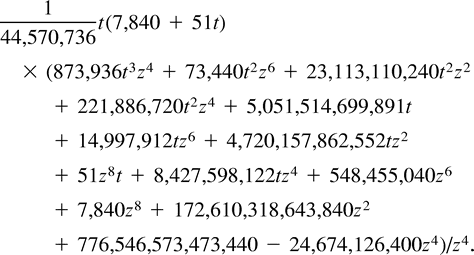
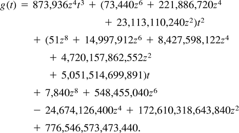
Example C is not symmetric either, and the most parsimonious tree for these data is (12)(34), inducing a total of 12 changes. Again, the two other trees, (13)(24) and (14)(23), attain lower likelihood values, so we describe the turning points of the likelihood function on the tree (12)(34). Employing Lagrange multipliers, we found one family of solutions, which is the rather simple curve in equation (5) . This curve intersects the parameter space in one connected region, 0 ≤ z ≤ 14. Combining the constraints of nonnegative edge weights, we are further restricted to the region 4 ≤ z ≤ 10. Thus, the points of the curve sol_c that satisfy 4 ≤ z ≤ 10 are the only candidates for maximization of the likelihood for data set (C). To verify this, we again employed both the Hessian technique and numeric hill climbing. The details are similar to those for data set (B), and we omit them.□

Conclusions

The goal of this research was to understand more about the likelihood surface for sequence data, especially the possible occurrence of multiple optima (local and global). In order to do this, we developed analytical techniques, including equations that represent ML points on trees and the direct computation of the first- and second-order derivatives of the likelihood function with respect to parameters of the model. These results are significant in their own right and could be developed further. We obtained closed-form ML solutions for certain data sets. At present, our ability to find such solutions is dependent on the exact platform and the version of the MAPLE software we are using. Our method is also very sensitive: small perturbations in the input can move us from instances that are easily solvable to ones where the system exhausts its memory and time resources without finding a solution. However, we believe that for four species, refining our techniques should make it possible to find closed-form solutions with general inputs. Given the importance of quartet-based tree reconstruction (Bandelt and Dress 1986 ; Strimmer and von Haeseler 1996 ; Wilson 1998 ; Ben-Dor et al. 1998 ; Erdos et al. 1999 ), such a result is highly desirable. It may be possible to extend this to five or six species. However, even in the two-state model, n species give rise to a system of 2ⁿ − 2n + 1 polynomial equations in that many variables. Such exponential size systems would not be easily solvable for large values of n.

In all of the examples we found with a continuum of ML points, the corresponding probability s_α is fixed for every split α with nonzero observed value ŝ_α > 0, so the likelihood function L attains a constant value on these curves. We expect that it is unlikely that there exist examples with a continuum of ML points where all the observed values of ŝ_α are nonzero. It may be argued that for long enough sequences on four taxa, real data with any of the eight components of ŝ = ø is not very likely. On the other hand, for larger values of n, most ŝ_α values will be 0, because it is not possible in practice to sequence genomic data of length exceeding 2ⁿ sites, let alone 4ⁿ. Furthermore, for n > 30, the genome is just not long enough.

ML phylogenetic analysis poses a number of intriguing open problems, in both the computational and the biological contexts. It is still unknown whether the problem is NP hard for a unary representation of the input. For example, the observed spectrum ŝ which is represented in binary as [14, 0, 0, 3, 0, 2, 1, 0] would be [11111111111111, 0, 0, 111, 0, 11, 1, 0] in unary, which is a much expanded representation. This unary representation is the natural one, given aligned DNA or amino acid sequences as the input. When the input is represented in binary form, Tuffley and Steel (1997) have shown NP hardness (via a reduction to maximum parsimony). Current ML packages use heuristics to prune the tree space, followed by hill climbing to converge to the optimal edge weights in each tree. Are there better approaches in cases where multiple ML points are not a problem? Can we characterize what such data sets look like? It would be very useful to identify special cases where ML is easy to compute and to devise efficient algorithms for them.

Our (A) and (B) examples have only four site patterns (nonzero entries in ŝ) to estimate five edge lengths. Thus, one may argue that these examples are not realistic, and it would be misleading to make recommendations about phylogenetic algorithms based on such example's. However, our data set (C) has six site patterns — one more than the number of parameters to estimate, so if the criterion for “interesting data” is more site patterns than edges, data set (C) certainly meets this criterion. The 27 additional data sets with six site patterns and ML solutions similar to (C), as well as the four data sets with eight site patterns and two ML points, also meet this criterion.

From a biological viewpoint, it is essential to know as much as possible about the properties of the likelihood surface. Knowing that multiple optima can occur is important for computational strategies to locate the ML tree. The most obvious strategy is to use multiple starting points. Rogers and Swofford (1999) have employed this approach, although this increases the computational cost (and may still miss ML points with small areas of attraction or in cases where there are exponentially many local maxima). It is also important now to describe properties of the surface, including the zones of attraction that lead to a given optimum (see Charleston 1995 ).

It has been assumed that with real data, multiple optima are unlikely. The present results show that this assumption requires more thorough analysis. Simulations are of limited use in estimating the frequency of multiple optima that might occur with biological data. For example, simulations are normally carried out on data generated on a tree by a simple Markov process, followed by studying the distribution of ML values (or other optimality criteria) on trees. Not surprisingly, trees are a reasonable description of data generated on trees.

There are, however, several reasons why a tree is an incomplete description of biological data. There may be genuine historical signals in addition to a tree from: recombination between different genes of viral strains, gene conversion between paralogous genes, and lateral (horizontal) transfer of genes between species (see Page and Holmes 1998 ). Even in the absence of these mechanisms, there are other processes that will lead to additional signals in the data if the mechanism of evolution is incorrect and/or incomplete. These include nonstationarity with some sequences changing nucleotide and amino acid composition, similar selection (adaptation) on different lineages, sites that are assumed to be variable but are unable to evolve due to functional constraints, and changes in the sites that are free to vary throughout the tree (the covarion model; Lockhart et al. 1999 ). For all these reasons, it is not possible to generalize from data simulated under a strict tree model to biological data, and consequently there is a need for further analytical investigation, as well as empirical studies with biological sequence data.

In the present work, we restricted our synthetic data sets to be conservative (they do not lend to any infinite distances) so they could be generated by a mixture of Markov processes. Real biological data do sometimes fail to be conservative, and this reinforces our conclusion that our present examples are in some sense biologically realistic. Clearly, much more work is required on the problem of multiple maxima and algorithms that work well with real data.

Masami Hasegawa, Reviewing Editor

1

Keywords: maximum likelihood phylogenetic trees likelihood surface multiple optima Hadamard conjugation

Table 1 Three Data Sets (A, B, and C) that Yield a Continuum of Maximum-Likelihood Trees

Table 2 Families of Data with Eight Site Patterns that Yield Multiple Maximum-Likelihood (ML) Trees

Fig. 1.—The tree T′ = (12)(34) and its edges

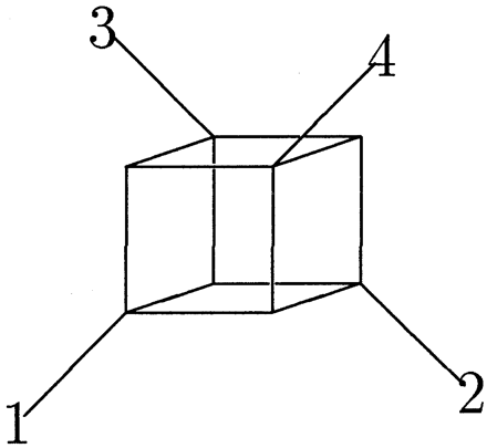
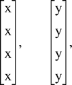
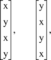
Fig. 2.—The order 4 splits space. There are 2⁴⁻¹ − 1 = 7 ways to partition {1,2,3} nontrivially. Each partition corresponds either to a single edge in the structure or to 4 parallel edges

Fig. 3.—Three maximum-likelihood weighted trees for data set (A)

Fig. 4.—The two regions of maximum likelihood for data set (A). In sol_I, the sum q₃ + q₁₂₃ of the edge lengths to taxon 3 (q₃) and to taxon 4 (q₁₂₃) is a constant. As the length q₃ decreases, the length q₁₂₃ increases, and vice versa. For sol_II, we have a similar behavior with respect to the edge lengths q₁ and q₂. See the text for more information

Fig. 5.—Two maximum-likelihood weighted trees for data set (B)

Fig. 6.—The two regions of maximum likelihood for data set (B)

We thank to Mike Steel for useful discussions and suggestions, and Katherina Huber, Sagi Snir, Mike Steel, and the anonymous referees for helpful comments on earlier versions of this manuscript. An extended abstract of this paper appeared in Proceedings of the fourth Annual International Conference on Computational Molecular Biology (RECOMB),April 2000. B.C. is on sabbatical leave from the Computer Science Department, Technion, Haifa, Israel, and was partially supported by the Fund for Promotion of Research at the Technion.