SIBELIUS-DARK: a galaxy catalogue of the local volume from a constrained realization simulation

ABSTRACT

We present sibelius-dark, a constrained realization simulation of the local volume to a distance of 200 Mpc from the Milky Way. sibelius-dark is the first study of the ‘Simulations Beyond The Local Universe’ (sibelius) project, which has the goal of embedding a model Local Group-like system within the correct cosmic environment. The simulation is dark-matter-only, with the galaxy population calculated using the semi-analytic model of galaxy formation, galform. We demonstrate that the large-scale structure that emerges from the sibelius constrained initial conditions matches well the observational data. The inferred galaxy population of sibelius-dark also match well the observational data, both statistically for the whole volume and on an object-by-object basis for the most massive clusters. For example, the K-band number counts across the whole sky, and when divided between the northern and southern Galactic hemispheres, are well reproduced by sibelius-dark. We find that the local volume is somewhat unusual in the wider context of ΛCDM: it contains an abnormally high number of supermassive clusters, as well as an overall large-scale underdensity at the level of ≈5 per cent relative to the cosmic mean. However, whilst rare, the extent of these peculiarities does not significantly challenge the ΛCDM model. sibelius-dark is the most comprehensive constrained realization simulation of the local volume to date, and with this paper we publicly release the halo and galaxy catalogues at z = 0, which we hope will be useful to the wider astronomy community.

methods: numerical, galaxies: formation, cosmology: theory, dark matter, large-scale structure of Universe

1 INTRODUCTION

Over the past few decades cosmological computer simulations have become an increasingly effective tool for advancing our understanding of structure and galaxy evolution in the Universe (see Frenk & White 2012; Vogelsberger et al. 2020, for comprehensive reviews). The Lambda cold-dark-matter model (ΛCDM), frequently referred to as the standard model, is the leading paradigm to describe the nature of the cosmos. Structure formation proceeds from primordial density fluctuations in a ‘bottom up’ manner, with low-mass structures (referred to as haloes) collapsing first and larger structures forming later (Davis et al. 1985). The traditional goal of ΛCDM cosmological simulations, such as the recent Horizon-AGN (Dubois et al. 2014), Magneticum (Hirschmann et al. 2014), EAGLE (Schaye et al. 2015) and IllustrisTNG (Pillepich et al. 2018) simulations, has been to produce a ‘random’ representative patch of the Universe that can be statistically compared to the one we observe, in terms of the properties of the large-scale structure, clustering statistics, the galaxy abundance and diversity, etc. However, whilst these simulated universes might reflect the observed Universe statistically, they do not contain the specific objects (such as the Local Group, or the Virgo and Coma clusters), embedded within the correct large-scale structure, that we actually observe. There remains an underlying tension between an observational data set, which is subject to cosmic variance, and the ensemble mean predictions from cosmological simulations.

How then can one determine the nature of specific objects within our Universe? Is it possible to deduce unambiguously the evolutionary pathways that led them to the point at which we observe them? One method that broadly attempts to answer this question involves a brute force approach: scouring large random ΛCDM cosmological simulations for model analogues that are as similar as possible to the particular object in question. For example, to examine the nature of the Milky Way and the Local Group, our most robust observational environment to study small-scale astrophysics, studies such as the ELVIS (Garrison-Kimmel et al. 2014, 2019) and APOSTLE (Sawala et al. 2016) projects have simulated, in exquisite detail, halo pairs of Local Group analogues extracted from large random ΛCDM cosmological simulations. Such studies have made meaningful advancements on our understanding of galaxy formation physics, particularly in relation to the so-called small-scale tensions between N-body (i.e. dark-matter-only) simulations of the ΛCDM model and observations (see Bullock & Boylan-Kolchin 2017, for a review), such as the core/cusp problem (Flores & Primack 1994; Moore 1994), the missing satellites problem (Klypin et al. 1999; Moore et al. 1999) and the ‘too big to fail’ problem (Boylan-Kolchin, Bullock & Kaplinghat 2011). Solutions to these problems based on cosmological hydrodynamics simulations of Local Group analogues have been proposed by Sawala et al. (2016).

However, whilst one can infer from studies using this brute force approach as to the prevalence of particular types of objects within the context of ΛCDM, for example, of a Local Group-like system, one cannot adequately ascertain the nature of the Local Group, as the non-linear formation of structure within our Universe allows an almost infinite number of evolutionary pathways towards the same end point. To truly probe the nature of our Local Group from cosmological simulations, or indeed of any particular object that we observe, it must be simulated within the correct cosmological environment, rather than a random one. This is the goal of ‘constrained realization’ simulations.

A constrained realization simulation has a focused objective: to deliberately construct a set of ΛCDM initial conditions that will evolve into the particular large-scale structure distribution of the observed local volume. Thus, the full phase-space distribution of the observed individual clusters, filaments, and voids in the local volume will each be reproduced by their model analogues, at the correct location, within the simulation. Simulations of this nature can go beyond asking questions such as how prevalent particular observed structures are in the context of ΛCDM, to predicting more accurately the particular formation pathways of the structures in the local volume with which we are so familiar, such as the Virgo cluster, the Coma cluster, and of course the Local Group.

The initial conditions for a constrained realization simulation can be derived from two related approaches. In the first, the initial density field is inferred from a data set of galaxy redshifts or radial peculiar velocities using the ideas pioneered by Bertschinger (1987) and Hoffman & Ribak (1991). Examples of such simulations include those by Mathis et al. (2002), the ‘Constrained Local UniversE Simulations’ (clues; Yepes, Gottlöber & Hoffman 2014; Carlesi et al. 2016) project, the ‘Constrained LOcal & Nesting Environment Simulations’ (clones; Sorce et al. 2021) project, the ‘ELUCID simulation’ (Wang et al. 2016), and the ‘High-resolution Environmental Simulations of The Immediate Area’ (hestia; Libeskind et al. 2020) project. In the second approach, the initial conditions are derived using Bayesian inference through physical forward modelling with a Hamiltonian Monte Carlo sampling approach, such as in the simulations by Wang et al. (2014), or the ‘Bayesian Origin Reconstruction from Galaxies’ (borg) project (Jasche & Wandelt 2013). Each technique can only constrain the density field above non-linear scales. Thus, the small-scale properties of the initial conditions remain random. However, for random realizations of the small-scale features, massive objects formed within constrained realization simulations, for example the Virgo cluster, retain consistent properties at the 10–20 per cent level (Sorce et al. 2016b), and similarly the Coma cluster (Jasche & Lavaux 2019), indicating that their formation is largely dictated by much larger scales. Thus, the scatter among random realizations that are constrained at the linear scale is substantially smaller, by a factor of 2–3 on scales of 5 h⁻¹ Mpc, than that found for random simulations (Sorce et al. 2016a), which allows us to zero-in on the most plausible evolutionary pathways of particular objects within the local volume.

Here we present sibelius-dark, the first of the ‘Simulations Beyond The Local Universe’ (sibelius) project (Sawala et al. 2022). The sibelius project has the goal of connecting the Local Group to the local environment by embedding a Local Group-like analogue within the correct large-scale structure produced by the borg algorithm. It encompasses, at high resolution, the constrained large-scale structure out to a distance 200 Mpc from the Milky Way, and so includes well-known clusters such as Virgo, Coma, and Perseus. Additionally, at the centre of sibelius-dark there is a Local Group-like halo pair with the correct dynamics. The simulation is dark-matter-only. The galaxy population, which matches well many observational data sets both statistically and, in particular, massive clusters, is calculated using the semi-analytic model of galaxy formation, galform (Lacey et al. 2016). Often, previous works using constrained initial conditions have focused on the evolution and properties of individual objects within the local volume, such as the Local Group (e.g. Libeskind et al. 2011; Carlesi et al. 2020) or the Virgo cluster (e.g. Sorce et al. 2021), or have simulated the local volume as a whole, yet to much smaller radii (≲8000 km s⁻¹, e.g. Mathis et al. 2002; Klypin et al. 2003). Here, the combination of such a large constrained region at high resolution that is self-consistently connected to the evolution Local Group makes sibelius-dark the most comprehensive constrained realization simulation to date.

The layout of this paper is as follows. In Section 2 we present an overview of the method for generating the sibelius constrained initial conditions, describing how a Local Group-like object is embedded within the large-scale structure produced by the borg algorithm. We then demonstrate how well the sibelius-dark halo and galaxy population match the data on a statistical level in Section 3.1, and on a cluster-by-cluster level in Section 3.2. In Section 3.3 we further investigate how well the sibelius-dark analogues of the Virgo and Coma clusters match the data, and make predictions for the location and observability of their ‘splashback radius’ in Section 3.3.3. The nature of the Local Group analogue at the centre of the volume is explored in Section 3.4. Finally, we discuss our results and conclude in Section 4. In Section  A we present the details of how to access the sibelius-dark data at z = 0, which we make public with the publication of this paper.

2 METHOD

2.1 Generating phase information to construct a constrained realization of the local volume and the Local Group

The aim of the sibelius project is to construct Lambda-Cold-Dark-Matter (ΛCDM) initial conditions for a simulation that will evolve into the observed density and velocity fields of our local volume (i.e. to a distance d_MW ≲ 200 Mpc from our Milky Way), with a correctly placed and suitably representative Local Group analogue at its centre. Typically, representative cosmological simulations assume periodic boundary conditions. However, as the local volume is clearly non-periodic, the constrained phase information that describes the local volume is instead embedded within a larger periodic parent volume, L = 1 Gpc on a side. Therefore sibelius-dark, and all subsequent sibelius simulations, are performed using the ‘zoom-in’ technique, whereby only a region of interest is resimulated at high resolution, with the remainder of the volume being populated by low-resolution elements. We note that the initial conditions for sibelius-dark, as with all zoom-in resimulations, are designed to remain ‘uncontaminated’ through the course of the simulation, i.e. a sufficiently large initial volume is populated with high-resolution particles such that no low-resolution particles enter the high-resolution region of interest (in our case a sphere with radius 200 comoving Mpc from the simulated Milky Way position at z = 0) at any time.

In the sibelius setup, the fiducial observer is the centre of the parent volume ([x, y, z] = [500, 500, 500] Mpc). The ‘constrained’ phase information propagates out to a radius of 200 Mpc from this point (≈5 per cent of the total volume of the parent box), with the remainder of the volume being filled with random, or otherwords unconstrained, phase information. The initial conditions are designed such that there is no sharp boundary in the phase information at the edge of the constrained region, and the cumulative phase information through the entirety of the volume remains statistically consistent with ΛCDM.

The phase information that generates the initial density field is constructed in two distinct steps: the linear and mildly non-linear modes that govern the formation of the large-scale structure are produced using the ‘Bayesian Origin Reconstruction from Galaxies’ (borg) algorithm (Jasche & Wandelt 2013; Jasche & Lavaux 2019). The modes that govern the formation of systems at the size of the Local Group are largely dictated on scales below those included in the borg constraints (Sawala et al. 2021), and thus are included after, via a random shuffling of the smaller scale modes (Sawala et al. 2022). We briefly summarize these two steps below.

2.1.1 The borg algorithm

borg is a fully probabilistic inference algorithm designed to reproduce the 3D cosmic matter distribution from local galaxy surveys at linear and mildly non-linear scales. It incorporates a physical model for gravitational structure formation within the inference process itself, connecting the initial density field to the evolved large scale structure via a particle mesh, turning the task of analysing the present non-linear galaxy distribution into a statistical initial conditions problem. The result is a highly non-trivial Bayesian inverse problem (Kitaura & Enßlin 2008; Enßlin, Frommert & Kitaura 2009), requiring the exploration of a very high-dimensional and non-linear space of possible solutions to the initial conditions problem from incomplete observations (which are flux-limited and missing at some locations, e.g. in the Zone of Avoidance). Samples of the posterior distribution are obtained via an efficient implementation of the Hamiltonian Markov Chain Monte Carlo (MCMC) method. The algorithm self-consistently accounts for observational uncertainty such as noise, survey geometry, selection effects, and luminosity-dependent galaxy biases (full details of the process are described in Jasche & Wandelt 2013).

The limiting mode/scale the borg algorithm can constrain is dependent on the resolution of the particle mesh used for the gravitational structure formation simulation. Here, the analysis consists of 256³ grid nodes within a cubic Cartesian domain of side length L = 1000 Mpc, resulting in a total of ≈1.6 × 10⁷ inference parameters for the Bayesian analysis, corresponding to the amplitudes of the primordial density fluctuation at the respective grid nodes. The inference procedure therefore yields constrained realizations with a resolution of ≈3.91 Mpc (for full details see Jasche & Lavaux 2019). Although coarse, this resolution is sufficiently adequate to resolve galaxy clusters, concentrations, and voids of the local volume.

The input to the borg algorithm is the observed 3D density field, inferred in this instance from the 2M++ galaxy sample (Lavaux & Hudson 2011).¹ However, being Bayesian, borg cannot tell us the ‘true’ initial density field for this data set, but instead the most probable initial density fields given the observational constraints. For sibelius-dark we settled on iteration 9350 of the MCMC chain (Sawala et al. 2022), as, of the most probable realizations of the entire constrained volume, it best reproduced the masses and positions of the nearby Virgo and Fornax clusters relative to the Milky Way. An alternative choice of realization would result in a very similar constrained region as a whole, but will contain differences in the overall dark matter distribution and the masses of individual dark matter haloes. Future work will investigate the level of these differences on the halo and galaxy populations.

To demonstrate how well the non-linear structure of the local volume has been encapsulated via the borg reconstruction, Fig. 1 shows the dark matter distribution of the sibelius-dark volume in six spherical shells centred on the Milky Way. These are presented as all sky maps in a Mollweide projection in the galactic coordinate system, and cover the entirety of the constrained region (d_MW < 200 Mpc). Highlighted are some familiar structures: from our nearest cluster neighbours, Virgo and Fornax, to the concentrations of Hydra, Centaurus, and Norma, thought to make up the ‘Great Attractor’, as well as the dominant wall of Perseus-Pisces, the Coma supercluster and the Hercules superclusters. In addition to the concentrations of structure, prominent underdense voids are also visible. Overplotted in red are the galaxies from the 2M++ galaxy sample (Lavaux & Hudson 2011), which map extremely well to the underlying dark matter density field (see also Jasche & Lavaux 2019, for more analysis of the borg constraints).

Figure 1.

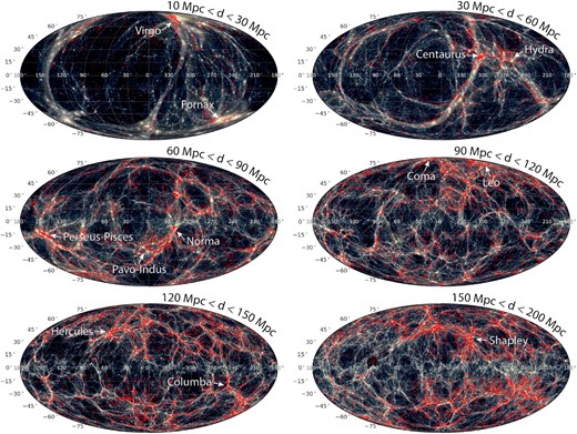
The dark matter distribution of the entire sibelius-dark volume (d_MW ≤ 200 Mpc), viewed in six spherical shells centred on the Milky Way (blue/green). Each slice is presented as an all-sky-map in a Mollweide projection using the Galactic coordinate system. Overplotted as red points are the galaxies from the 2M++ galaxy sample (Lavaux & Hudson 2011), demonstrating just how well the non-linear structure of the local volume has been encapsulated in the borg reconstruction. The locations of twelve famous clusters/concentrations are also highlighted.

Taking this one step further, we also include Fig. 2, which compares the inferred galaxy distribution of sibelius-dark in redshift space to a famous slice of the CfA redshift survey (Huchra et al. 1983), demonstrating again how well the borg constraints have captured the unique structure of our local volume.

Figure 2.

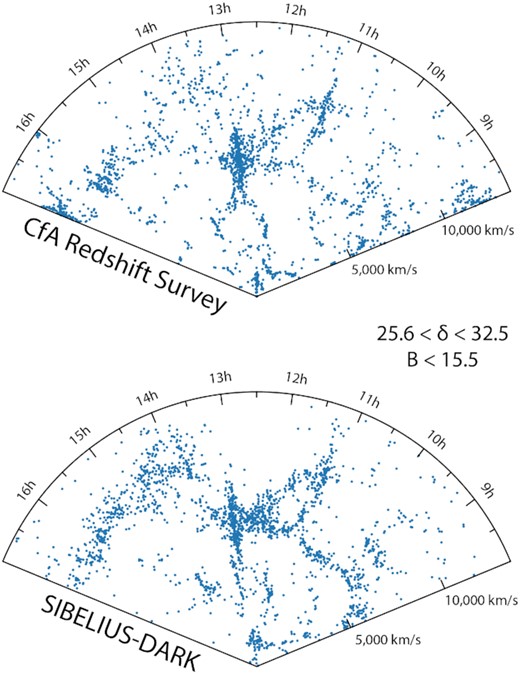
The top panel shows the distribution of galaxies in redshift space brighter than B < 15.5 from a famous slice of the CfA redshift survey (8h < RA < 17h & 25.6° < DEC <32.5° & 0 km s⁻¹ <v_r < 14, 500 km s⁻¹; Huchra et al. 1983). Below is the same slice from the inferred sibelius-dark galaxy population, demonstrating how well the borg constraints have captured the unique structure of the local volume.

2.1.2 Embedding a Local Group within the borg constraints

As mentioned above, the constrained phase information produced by the borg algorithm is limited to scales larger than the mesh size of ≈3.91 Mpc, a scale greater than those important for the formation of ∼10¹² M_⊙ haloes (λ_cut ≈ 1.62 Mpc; Sawala et al. 2021). Therefore the smaller scale phase information at the location of the Local Group currently remains random. In order to embed a Local Group-like system at the centre of the sibelius volume, we must therefore supply additional phase information. To do this, we leave the larger scale phases set by the borg constraints fixed, and then perform an exploration of the smaller scale phases within the 16 cMpc cubic region surrounding the Local Group location (i.e. the centre of the box). That is, we randomize the phases below 3.2 cMpc within the central 16 cMpc cubic region² until a system with accurate Local Group-like properties forms at the correct location. This results in multiple realizations that share the same large-scale phase information of the borg constraints, but differ substantially in their halo populations at lower masses (a method similar to the original CLUES project; Yepes et al. 2014).

Sawala et al. (2022) performed 60 000 low-resolution simulations randomizing the phases below 3.2 cMpc within the central 16 cMpc cubic region of the same borg realization. These variations were then probed for a dark matter halo pair that is no more than 5 Mpc from the centre of the box, and satisfies at least a ‘loose’ criteria for a Local Group-like system (see Table 1), i.e.

• There is no third system more massive than the Milky Way within 2 Mpc of the Local Group centre.

• The combined mass of the Milky Way and M31 falls within the range (1.2–6) × 10¹² M_⊙, and the ratio of the Milky Way halo mass with respect to the M31 halo mass is between 0.4 and 5.

• The relative distance between the Milky Way and M31 is between 500 and 1500 kpc.

• The relative radial velocity between the Milky Way and M31 is between −200 and 0 km s⁻¹ and the relative tangential velocity between the pair is less than 150 km s⁻¹.

• M31 is oriented at the right location on the sky when viewed from the Milky Way (to within an angular separation of 45°).

From the 60 000 simulations, 2309 contained a halo pair that satisfied this loose criteria (with the orientation on the sky being the most restrictive factor). When we refined this selection to a ‘strict’ criterion (see again Table 1), based on the most recent observational limits, we were reduced to no suitable candidates from the 60 000 runs. To avoid simply making more attempts in the hope of eventually finding a good Local Group, we instead took the nine most suitable candidates and resimulate each of them 1000 times, now only randomizing the scales below 0.8 cMpc, which serves to slightly perturb their properties. Of these resimulations, three systems then fulfilled the strict criteria, one of which is used here for sibelius-dark. The full details of this embedding process is presented in Sawala et al. (2022).

Table 1.

The ‘Loose’ and ‘Strict’ criteria a halo pair must satisfy to be classified as a Local Group, used for generating the sibelius-dark initial conditions (see Section 2.1.2 and Sawala et al. 2022). From left to right, the total halo mass of the MW+M31, their mass ratio, relative distance, radial velocity, tangential velocity, and angular separation from the observed location of M31 on the sky. The final two columns show how many candidates (with and without orientation constraint) satisfy each criteria from the 60 000 exploration runs performed in Sawala et al. (2022).

Criteria	Mtot	|$\frac{M_{\mathrm{MW}}}{M_{\mathrm{M31}}}$|	d	vr	vt	δ	|$N[M_{\mathrm{tot}},\frac{M_{\mathrm{MW}}}{M_{\mathrm{M31}}},d,v_{\mathrm{r}},v_{\mathrm{t}}]$|	|$N[M_{\mathrm{tot}},\frac{M_{\mathrm{MW}}}{M_{\mathrm{M31}}},d,v_{\mathrm{r}},v_{\mathrm{t}},\delta]$|
	(1012 M⊙)		(Mpc)	(km s−1)	(km s−1)	(°)
‘Loose’	1.2 → 6	0.4 → 5	0.5 → 1.5	−200 → 0	<150	<45	6385	2309
‘Strict’	2 → 4	1 → 2	0.74 → 0.8	−109 → −99	<40	<15	1	0

Naturally, the embedment process described above does not guarantee that the Local Group, or more specifically the Milky Way (i.e. the desired observer), will go on to form at exactly the centre of the parent volume at redshift z = 0 ([x, y, z] = [500, 500, 500] Mpc), i.e. the location of the fiducial observer as defined by the borg constraints. The sibelius-dark Milky Way is located at coordinates [x, y, z] = [499.343, 504.507, 497.311] at redshift z = 0, indicating it has drifted slightly outwith this limit, at a distance 5.3 Mpc from the centre of the parent volume. Yet to remain more consistent with the observations, for this study the observer is set to be the location of the simulated Milky Way at z = 0, and not the centre of the parent volume. This has very little impact on the results, however; for example the distance to the simulated Virgo cluster is changed by only ≈7 per cent depending on the observing location selected, and the distance to the simulated Coma cluster by less than 1 per cent.

2.2 Numerical setup

2.2.1 Initial conditions

The ΛCDM initial conditions for sibelius-dark were generated using first order (Zel’dovich) Lagrangian perturbation theory as set out by Jenkins (2010), calculated down to redshift z = 127. The displacement field for the zoom region is computed using two concentric meshes each of size 15360³, centred on the middle of the parent volume. The top level mesh covers the entire domain (L = 1000 Mpc) and the second mesh just covers the high-resolution region (L = 500 Mpc). The second mesh, while not strictly necessary to reach the particle Nyquist frequency in the zoom region, improves both the accuracy and the fidelity with which the Panphasia phase information is reproduced on the smallest length scales. A more in depth discussion of the initial conditions generation for sibelius can be found in Sawala et al. (2022).

Generating the initial conditions was performed using 183 compute nodes of the COSMA-7 DiRAC facility hosted by Durham University and required 91.5 TB of run-time memory. The L = 1000 Mpc volume is sampled by 131 billion (⁠|$N_{\mathrm{p}}^{3}=5078^{3}$|⁠) collision-less dark matter particles, less than 1 per cent of which are low-resolution boundary particles, with a high-resolution particle mass of 1.15 × 10⁷ M_⊙. The comoving gravitational softening length is set as ϵ_CM = 0.05 × (L/N_p) = 3.32 ckpc and the maximum physical softening length is ϵ_phys = 0.0022 × (L/N_p) = 1.48 kpc, following Ludlow et al. (2020). The mass resolution and gravitational softening lengths were chosen to match that of the upcoming eagle-xl model (the successor to the eagle model; Schaye et al. 2015), to allow for an optimal comparison between sibelius-dark and later hydrodynamical resimulations of the sibelius volume.

The combination of a large volume and a comparatively high resolution will make sibelius-dark a useful tool even when the constrained aspect of the simulation is not considered. For context, the resolution of sibelius-dark is comparable to that of the Millennium-II simulation (within ≈20 per cent; Boylan-Kolchin et al. 2009) yet has ≈13 times more volume; shares the same number of particles as the P-Millennium simulation (Baugh et al. 2019) at ≈13 times higher resolution (yet has ≈15 times less volume); and contains many massive clusters sampled by more particles than the majority of the phoenix (Gao et al. 2012) cluster sample (there are |${\approx}235\, 000\, 000$| particles within r200c of the sibelius-dark Perseus cluster).

The simulation adopts a flat ΛCDM cosmogony with parameters inferred from analysis of Planck data (Planck Collaboration XVI 2014): |$\Omega _\Lambda =$| 0.693, Ω_m = 0.307, Ω_b = 0.04825, σ₈ = 0.8288, n_s = 0.9611, and H₀ = 67.77 km s⁻¹ Mpc⁻¹.

2.2.2 The swift simulation code

The simulation was performed using swift (Schaller et al. 2018),³ an open source coupled gravity, hydrodynamics, and galaxy formation code. swift exploits task-based parallelism within compute nodes themselves, and interacts between compute nodes via MPI using non-blocking communications, resulting in excellent strong- and weak-scaling for cosmological calculations out to many tens of thousands of compute nodes (Schaller et al. 2016). The short- and long-range gravitational forces are computed using a 4th-order fast multipole method (e.g. Cheng, Greengard & Rokhlin 1999) and particle-mesh method solved in Fourier space, respectively, with an imposed adaptive opening angle criterion similar to the one proposed by Dehnen (2014). For this project, swift was run using only its N-body solver.

sibelius-dark was run on 160 compute nodes (using 320 MPI ranks for a total of 4480 compute cores) of the COSMA-7 DiRAC facility⁴ hosted by Durham University, for a total of 3.5 million CPU hours over 14 845 time-steps. We note, however, that the version of swift used did not exploit a domain decomposition algorithm tailored for zoom simulations. Up-coming code improvements in this direction are expected to reduce the required CPU time for such a simulation by at least 25 per cent.

2.3 Post-processing

Through the course of the sibelius-dark simulation 200 ‘snapshots’ were stored between redshifts z = 25 and z = 0, spaced linearly in the logarithm of the scale factor. The snapshots were post-processed to produce catalogues of Friend-Of-Friends (FOF) groups, using a linking length of 0.2 times the mean interparticle separation, and to produce catalogues of bound subhaloes using a heavily modified⁵ version of the publicly available ‘Hierarchical Bound-Tracing’ (hbt+) algorithm (Han et al. 2012, 2018). As a final step, the merger trees of these dark matter subhaloes were constructed using the dhalos algorithm described by Jiang et al. (2014). The combination of snapshots, dark matter subhalo catalogues, and merger trees serve as input to semi-analytic models of galaxy formation to produce mock galaxy catalogues, described in the next section. Our high cadence between outputs is necessary to capture accurately the evolution of dark matter haloes, as each snapshot is separated by less than the freefall time of the overdensities, and comfortably exceeds the recommended number of outputs required for use with semi-analytic models (e.g. Benson et al. 2012).

Due to their large size (5.3 TB each), all but 11 of the snapshots containing the complete particle data were deleted following the creation of the subhalo catalogues (the z = 5, 3, 2, 1, 0.5, 0.09, 0.07, 0.05, 0.03, 0.02, & 0 snapshots were kept).

Halo mass, denoted M_200c (m200crit in the public data base), is defined as the total mass enclosed within r_200c, the radius at which the mean enclosed density is 200 times the critical density of the Universe (i.e. 200ρ_crit). Dark matter haloes are populated by one (a central) or more (a central plus satellites) bound substructures (i.e. subhaloes). The total bound mass of the subhalo is denoted M_sub (Mbound in the public data base).

2.3.1 The semi-analytic model galform

To infer how the galaxy population of the sibelius-dark volume evolves, we use the semi-analytic model of galaxy formation, galform (Lacey et al. 2016). Semi-analytic models, or SAMs, are a computationally efficient method to describe the physical processes giving rise to the formation and evolution of galaxies. They are built upon the output of dark matter-only (DMO) N-body simulations, which offers the possibility of exploring galaxy evolution down to the smallest scales within extremely large cosmological volumes, such as sibelius-dark, at a fraction of the expense of a full hydrodynamical simulation. The downside of this method, compared to a full hydrodynamical simulation, is its simplicity. For example, SAMs are limited in their ability to explore the internal structure of galaxies, non-symmetric features, and intergalactic gas. Yet recent improvements to semi-analytic modelling do show reasonable agreement with hydrodynamical counterparts (Guo et al. 2016; Hou, Lacey & Frenk 2018, 2019). Moreover, the semi-analytic approach has a distinct statistical advantage: being computationally so inexpensive, it is possible to explore the parameter space of models thoroughly, resulting in an accurate calibration against many observational data sets with a strong predictive power.

The latest galform model of Lacey et al. (2016) includes a different initial mass function for quiescent star formation and starbursts, feedback from active galactic nuclei to suppress gas cooling in massive haloes, and a new empirical star formation law in galaxy discs based on the molecular gas content. In addition, there is a more accurate treatment of dynamical friction acting on satellite galaxies and an updated stellar population model. The magnitudes of galaxies in galform include the reprocessing of starlight by dust, leading to both dust extinction at ultraviolet to near-infrared wavelengths, and dust emission at far-infrared to sub-mm wavelengths. The absorption and emission is calculated self-consistently from the gas and metal contents of each galaxy and the predicted scale lengths of the disc and bulge components using a radiative transfer model (Lacey et al. 2011; Cowley et al. 2015; Lacey et al. 2016).

The simulation data used for this study, and that made available for public release (see Section  A), is not a light cone, it is the halo and galaxy catalogue at z = 0. Thus we have assumed a negligible evolution in the positions and properties of the sibelius-dark galaxies between z = 0.045 (the edge of the constrained region) and z = 0. We define the redshift of a galaxy as z = v_r/c, where v_r is the radial velocity (which includes the Hubble flow) and c is the speed of light, and we define the apparent magnitude as m = M + 5log₁₀(d/10), where d is the distance to the simulated Milky Way in pc and M is the absolute magnitude.

3 RESULTS

3.1 The halo and galaxy population of sibelius-dark

We begin with a statistical investigation of the sibelius-dark volume in its entirety, that is, a study of all galaxies out to a distance of d_MW ≤ 200 Mpc from the Milky Way. As a reminder, sibelius-dark was performed as a DMO simulation; the properties of the galaxies populating those dark matter haloes are computed in post-processing using the semi-analytic model galform (see Section 2.3.1).

At z = 0 sibelius-dark hosts 22 904 767 dark matter haloes with a mass in excess of M_200c ≥ 10⁹ M_⊙, which in turn host 33 220 267 bound dark matter subhaloes above the same mass threshold. Of these haloes, seven exceed M_200c ≥ 1 × 10¹⁵ M_⊙ (which is potentially an unusual amount, we discuss this more in Section 4), the most massive of which is located at approximately ≈77 Mpc from the Milky Way, the Perseus cluster, with a mass of M_200c = 2.72 × 10¹⁵ M_⊙. The distribution of halo and subhalo masses within three spherical volumes centred on the Milky Way are shown in Fig. 3. For a comparison, the distribution of halo and subhalo masses from the DMO eagle reference simulation (eagle-dark; Crain et al. 2015; Schaye et al. 2015; McAlpine et al. 2016), a (100 Mpc)³ unconstrained periodic volume, are also shown, with the ratio between the sibelius-dark volumes and the eagle-dark volume shown in the lower panels. We note that the eagle-dark simulation was performed using the same cosmology and at the same resolution as sibelius-dark. In addition, we re-post-processed the eagle-dark outputs using the hbt+ structure finder to remain consistent with the sibelius-dark catalogues.

Figure 3.

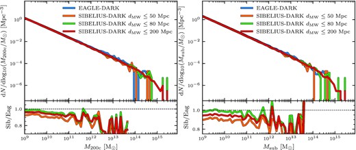
The halo (left-hand panel) and subhalo (right-hand panel) mass functions within three spherical volumes centred on the Milky Way. For comparison, the halo and subhalo mass functions of the unconstrained (100 Mpc)³ reference eagle DMO volume (eagle-dark), and the ratios to this volume (lower panels), are also shown. There are fewer haloes/subhaloes per unit volume in sibelius-dark compared to eagle-dark (≈2–10 per cent at 10¹⁰ M_⊙). The level of difference within each spherical volume directly reflects the volumes average density relative to the mean density (which the eagle-dark volume is at, see also Fig. 4), suggesting that the local volume, particularly the innermost 50 Mpc, is underdense relative to the cosmic mean.

Over the mass range we explore (≥10⁹ M_⊙), there are generally fewer haloes/subhaloes per unit volume within sibelius-dark compared to the eagle-dark volume. This deficit, in the range ≈2–10 per cent, is considerably larger than one would expect from sample variance alone at these scales (≈1 per cent at M_200c ≈ 10¹⁰ M_⊙; Sawala et al. 2021). Here, ‘sample variance’ refers to the expected level of scatter in the halo population depending on the initial Gaussian random field that went in to producing the initial conditions. However, it is important to realize that the level of sample variance measured from studies such as Sawala et al. (2021) are inferred from periodic cubic volumes that are fixed to the mean density. As the inner regions of sibelius-dark, and indeed our own local volume, are not guaranteed to reside at the mean density exactly, this creates an additional level of scatter when comparing to unconstrained simulations, such as eagle, which we refer to as ‘cosmic variance’.

The level of cosmic variance within sibelius-dark is most clearly demonstrated in Fig. 4, showing the density of matter, relative to the mean density, within shells (top) and increasingly larger spheres (bottom) centred on the simulated Milky Way. There are substantial variations in the average shell density depending on the volume being considered, rapidly changing between underdense and overdense regions correlating with the presence (and absence) of massive structures. Any one volume of the Universe is unique, but to give context we show the one, two, and three σ ranges of density fluctuations which one would expect in the confines of ΛCDM. These ranges are computed by performing the equivalent calculation from a sampling of 1000 randomly located R = 500 Mpc spheres within a 3.2 Gpc DMO simulation. With this context, the upper panel of Fig. 4 reveals three regions within the sibelius-dark volume that stand out as ‘unusual’: it is rare to have something as massive as the Virgo cluster so nearby, the density of the shells that collectively contain the Norma cluster and Perseus-Pisces superstructure is unusually high (and the voids that they create on either side are unusually underdense), and the shells towards the outer regions of the local volume are anonymously underdense (which could potentially be linked to the evacuated regions before the Shapley concentration). When considered more generally, the spherical volumes in the lower panel reveal that the local volume is largely ‘normal’, remaining within ΛCDM’s 1σ range. Yet we note that the spherical volumes typically always verge on the side of an underdensity, particularly at d_MW ≈ 50 Mpc and at the outskirts of the local volume (d_MW ≈ 175–200 Mpc) where an overall underdensity of ≈5 per cent is found, a 2σ deviation in ΛCDM (an underdensity that is consistently found across all the borg realizations, see fig. 10 of Jasche & Lavaux 2019). It is not until a distance of d_MW ≈ 400 Mpc that the volume recovers from this underdensity and stabilizes to the mean density, which is well into the unconstrained region of the parent volume.⁶ We would therefore require constrained initial conditions that go beyond our current limit of d_MW = 200 Mpc in order to see the true extent of this underdensity.

Figure 4.

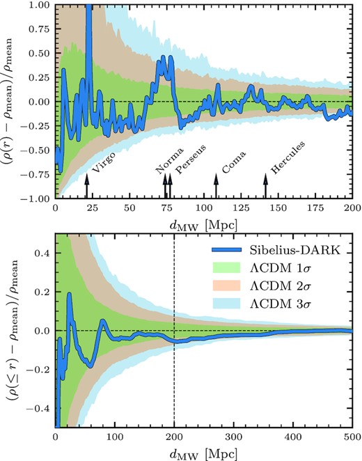
Total matter density, relative to the mean cosmic density (Ω_mρ_crit), within shells (top) and increasingly larger spheres (bottom) centred on the simulated Milky Way. In the upper panel we show the location of 5 sibelius-dark clusters. The vertical dashed line in the lower panel indicates the boundary of the constrained region, beyond this mark we enter the unconstrained parent volume. The shaded regions indicate the expected range of density fluctuations for ΛCDM, computed from 1000 random samplings of R = 500 Mpc spheres within a unconstrained 3.2 Gpc DMO volume. There is a large variation in the average density depending on the volume considered, which explains the systematic shifts of the halo/subhalo mass function in Fig. 3. At the boundary of the constraints, d_MW = 200 Mpc, our local volume is predicted to have an overall underdensity of ≈5 per cent, a ≈2σ deviation in ΛCDM.

Translating this back to the halo and subhalo mass functions in Fig. 3, it is then clear why, and to what level, there are systematic differences in the number of haloes relative to the unconstrained eagle-dark volume, which as a reminder is fixed to the mean density. Overall, this suggests that our local volume, particularly our most immediate neighbourhood (d_MW < 50 Mpc), is underdense relative to the cosmic mean. We discuss this more in Section 4.2.

3.1.1 The galaxy population

Turning now to the model galaxy population, Fig. 5 shows the luminosity function of galaxies at z = 0 in the three primary bands of the Sloan Digital Sky Survey (SDSS); g, r, and i. Here we include the model prediction both including and excluding the effects of dust extinction, and, to compare, data from the SDSS survey itself (Blanton et al. 2003). There is a general good agreement between the model prediction and the data, with only the brightest g-band galaxies being slightly overproduced by the galform model.

Figure 5.

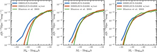
The g, r, and i-band luminosity functions of sibelius-dark galaxies at z = 0, both including (orange) and excluding (blue) the effects of dust extinction. Observational data in green is from the SDSS survey (errors as grey bands, but they are almost always smaller than the line width; Blanton et al. 2003).

Fig. 6 shows, from left to right, the predicted K-band luminosity function compared to observational estimates from Kochanek et al. (2001) and Driver et al. (2012), the galaxy stellar mass function (GSMF) compared to observational estimates from Li & White (2009) and Wright et al. (2017) and the central supermassive black hole mass–stellar bulge mass relation compared to the observational estimates from Sahu et al. (2019). The behaviour of the K-band magnitudes and the GSMF is similar between the model and the data, differing mostly in the normalization at the position of the ‘knee’, the area of the GSMF most sensitive to the particular implementation of stellar and AGN feedback (e.g. Bower, Benson & Crain 2012). This underprediction of intermediate mass galaxies (M_* ∼ 10¹⁰ M_⊙) seen in the model population relative to observational estimates is not unique to sibelius-dark, and is predicted also by the galform semi-analytic model performed on unconstrained volumes. For example, we overplot the equivalent galform GSMF using the same 100 Mpc eagle-dark volume that was used for Fig. 3 (see also the results from Guo et al. 2016; Lacey et al. 2016), which additionally demonstrates that the ensemble properties of galaxies from the sibelius-dark volume are predicted to be very similar to those within unconstrained volumes. It is likely that the discrepancy at the knee of the GSMF, at least in part, is due to how the stellar mass is estimated. Here the model stellar masses are directly measured, yet observationally they are inferred from SED fitting, the results of which depend on the stellar population synthesis model used, on assumptions about galaxy star formation histories and metallicity distributions, on the model for dust attenuation, and on the assumed initial mass function. When galform stellar masses are estimated using observational techniques, the normalization around the knee is boosted, bringing the prediction much closer to the observational estimates (e.g. Mitchell et al. 2013; Lacey et al. 2016). Finally, the relation between the mass of the central supermassive black hole and the mass of the stellar bulge matches extremely well to the recent observational data of Sahu et al. (2019).

Figure 6.

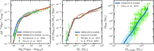
Left-hand panel: the K-band luminosity function at z = 0, both including (orange) and excluding (blue) the effects of dust extinction, compared to observational estimates from Kochanek et al. (2001) and Driver et al. (2012). Middle: the galaxy stellar mass function (GSMF) at z = 0, compared to observational estimates from Li & White (2009) and Wright et al. (2017). Overplotted as an orange dashed line is the galform GSMF from the eagle-dark 100 Mpc unconstrained volume, which demonstrates that the ensemble properties of galaxies within sibelius-dark are predicted to be very similar to those from unconstrained volumes. Right-hand panel: the central supermassive black hole mass–stellar bulge mass relation at z = 0, compared to the observational estimates from Sahu, Graham & Davis (2019). The line is the median value and the shaded region highlights the 10th to 90th percentile range.

3.1.2 Galaxy number counts

When considering the global characteristics of a model galaxy population, such as the stellar mass function, cosmic variance is often mitigated by calculating an ensemble average over many possible distributions of the large scale structure. One can then investigate how these average characteristics compare to our local observations in order to gain theoretical understanding. The power of sibelius-dark, as a constrained simulation, is that we can now directly compare to the particular large-scale structure distribution of our local volume, subject to the same biases in the same directions of the sky. This allows us to mimic observational surveys more directly, not only by applying the limitations of the instrument, but also by focusing on the same particular region of the sky that is surveyed. Here we demonstrate a direct comparison to the 2M++ and 2MRS all-sky galaxy samples (Lavaux & Hudson 2011; Huchra et al. 2012), and the SDSS survey, Data Release Twelve (SDSS-DR12; Ahumada et al. 2020).

The analysis in this section investigates galaxy number counts, both as a function of magnitude (n(m)) and as a function of redshift (n(z)). We estimate the variance (σ) for the galaxy counts using the ‘field-field’ error technique, whereby we compute the area-density of galaxies over n equal-area sub-fields (ρ_i) relative to the area-density of galaxies over the entire field we are considering (⁠|$\bar{\rho }$|⁠), i.e.

$$\begin{eqnarray*} \sigma ^2 = \frac{1}{n(n-1)} \sum ^{n}_{i=1} (\rho _i - \bar{\rho })^2, \end{eqnarray*}$$

(1)

(see Section 2.3 of Wong, Shanks & Metcalfe 2021, for more details). For Fig. 7 we define n = 12 equal area sub-fields covering the whole sky (excluding |b| < 15°), for Fig. 8 we estimate the field-field errors for the galaxy counts in the Galactic north and the Galactic south from the six sub-fields in the relevant hemisphere, and for Fig. 9 we divide the North Galactic Cap region into n = 6 equal area slices of right ascension.

Figure 7.

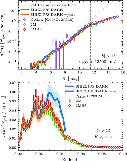
Top: K-band number counts (n(m)) of sibelius-dark galaxies both with (w/) and without dust extinction compared to the 2M++ and 2MRS galaxy samples and the GAMA survey. The galaxies from each data set are limited to those with v_MW < 13500 km s⁻¹ (d_MW ≲ 200 Mpc). We find excellent agreement between the model galaxies from the simulation and the observational data. Beyond K ≈ 11.5 the power-law slope shallows due to the limited volume we consider (this is demonstrated by the opaque crosses, which are the same GAMA data with no volume cut applied). Bottom: redshift distribution (n(z)) of galaxies with K < 11.5. Again, there is a good agreement between the simulation and the observations, with only a potential slight underabundance (≈20 per cent) of galaxies within sibelius-dark around z = 0.02. Errorbars and shaded regions in both panels are ‘field-field’ errors over n = 12 equal-area sub-fields covering the entire sky (see the text).

Figure 8.

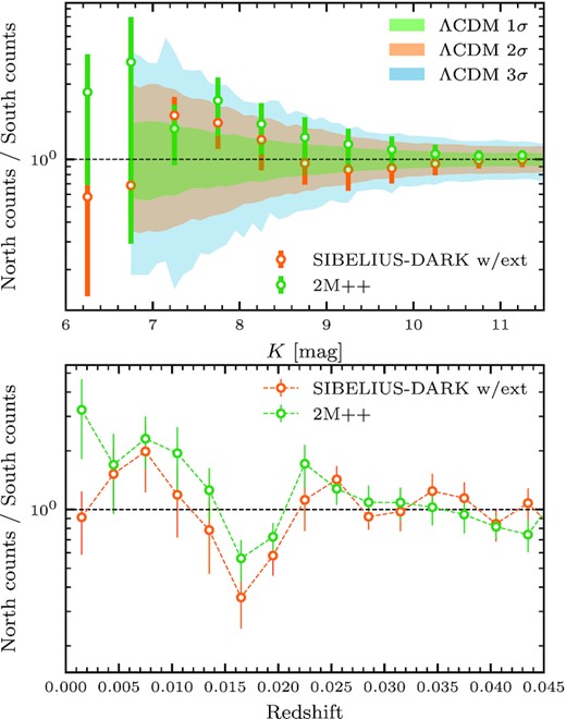
Similar to Fig. 7, now investigating the ratio of counts between galaxies in the Galactic north (b > 15°) and the Galactic south (b < −15°). Top: for both the simulation and the data we find faint galaxies (K ≳ 9) have approximately equal numbers between the two hemispheres, whereas brighter galaxies (K ≲ 9) are more abundant in the north relative to the south (by a factor of ≈2–3). For the brightest galaxies (K < 7) however, 2M++ galaxies remain northern dominated, whereas sibelius-dark galaxies are more equally split. By comparing to 1000 random samplings of the Millennium simulation, we find these behaviours are not unusual within a ΛCDM context, generally falling within the 1–2σ range. Bottom: the north/south ratio now considered as a function of redshift, which is particularly sensitive to the distribution of large scale structure. For example, there are more galaxies in the Southern hemisphere at z ≈ 0.017 due to the Perseus-Pisces superstructure. The generally good agreement between sibelius-dark and the data indicates a similar distribution of the large-scale structure.

Figure 9.

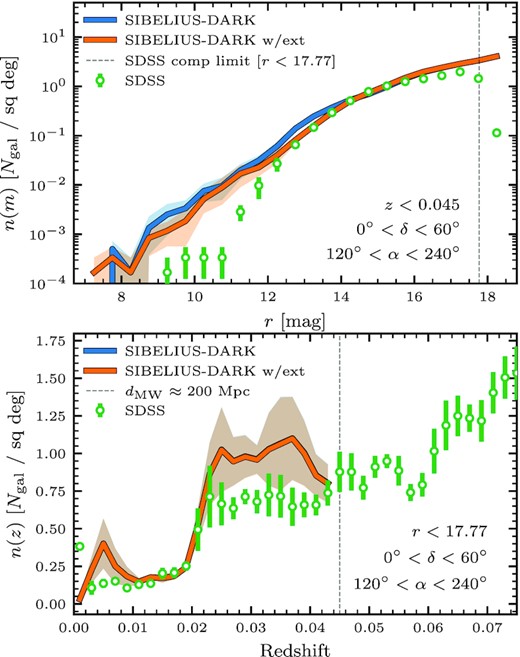
The layout of this figure is the same as Fig. 7, now showing the n(m) and n(z) distributions in the r-band for galaxies in the North Galactic Cap region (bounds detailed in figure) of the SDSS survey. In the upper panel only galaxies with z < 0.045 (d_MW ≲ 200 Mpc) are considered. In the lower panel only galaxies within the spectroscopic completeness limit for SDSS are considered (r < 17.77). Errors are ‘field-field’ errors over n = 6 equal-area slices of right ascension within the North Galactic Cap (see the text). Note in the lower panel the two sibelius-dark lines overlap.

The upper panel of Fig. 7 shows the K-band number counts of sibelius-dark galaxies compared to the 2M++ and 2MRS galaxy samples, the all-sky samples from which the borg constraints were derived. Given that the galaxies in both 2M++ and 2MRS go slightly deeper than d_MW = 200 Mpc (the boundary of the sibelius-dark constraints), we limit all model and observed galaxies to those with radial velocities less than v_MW < 13 500 km s⁻¹. In addition, we only consider galaxies at galactic latitudes |b| > 15° to minimize the effects of obscuration from the galactic disc in the data. We show the counts of sibelius-dark galaxies both with (w/) and without dust extinction to demonstrate the widest possible range in the semi-analytic model prediction. The n(m) counts reveal a familiar power-law behaviour, with the model galaxies from sibelius-dark being in excellent agreement, both for the slope and the normalization, with the galaxies in the 2M++ and 2MRS samples. Approximately just beyond the completeness limit of the data (K = 11.5) the sibelius-dark galaxies start to taper off, and continue with a shallower slope towards the faint end. To clarify why this is, we include galaxies from three complete fields of the GAMA survey (G09, G12 & G15; Baldry et al. 2018), which go much deeper in the K-band than 2MRS and 2M++ , but cover a much smaller area of the sky. We again find excellent agreement with the sibelius-dark prediction for the GAMA galaxies, both brighter and fainter than K = 11.5. The change in slope towards fainter galaxies is due to the limited volume that we are considering (d_MW < 200 Mpc), as the distant bright galaxies are simply not present to bolster the numbers of the nearby intrinsically faint galaxies. Indeed, if we were not to enforce the distance cut of v_MW < 13 500 km s⁻¹ to the GAMA data, the power-law slope continues uninterrupted beyond K = 11.5 (shown as opaque crosses).

Next we investigate how the model sibelius-dark galaxies and those from the 2M++ and 2MRS samples are distributed in redshift, which we show in the lower panel of Fig. 7. Here we only consider the galaxies within the completeness limit of the observational data (K < 11.5), and now no longer consider the galaxies from the GAMA survey (as they are not all sky). Both the counts of the observed galaxies and those from sibelius-dark rise and fall within a radius of 200 Mpc, coming to a peak between redshifts z = 0.02 and z = 0.03. There is good general agreement between the trend of the simulation and the trend of the observations, with the 2M++ and 2MRS galaxies often overlapping with the curves of sibelius-dark. However, there is potentially up to a ≈20 per cent deficit of sibelius-dark galaxies around z = 0.02 compared to the observations, which is approximately at the distance of the Perseus-Pisces and Norma superstructures.

Previously, in Fig. 7, we considered the galaxy distribution across the entire sky (excluding only the galactic plane, |b| > 15°). Yet we can also narrow our focus to particular sub-regions of the sky, in a test of homogeneity. Fig. 8 shows, again for the K-band, the ratio of the number of galaxies in the Galactic north (b > 15°) compared to those in the Galactic south (b < −15°), both for the 2M++ data and for sibelius-dark. For both data sets, the behaviour is generally similar over a wide range of magnitudes; galaxies fainter than K ≳ 9 have approximately equal numbers between the northern and Southern hemisphere, whereas brighter galaxies in the range 7 ≳ K ≳ 9 are more abundant in the north relative to the south (up to a factor of ≈2 for sibelius-dark and up to a factor of ≈2.5 for 2M++). It is the brightest galaxies in the 2M++ sample that show the largest difference between the two hemispheres, with 58 of the 79 galaxies brighter than K < 7 found in the Galactic north, whereas there are more sibelius-dark galaxies in the Galactic south in this regime. In future work it will be interesting to see how sensitive the number of bright galaxies between the northern and southern hemispheres is to the particular realization of the borg constraints.

To test the likelihood of such a north–south disparity for bright galaxies is in the context of ΛCDM, we use the Millennium simulation (MS-W7),⁷ a publicly available ΛCDM simulation with a volume ≈15 times greater than sibelius-dark. We perform 1000 random samplings of R = 200 Mpc spheres within the MS-W7 simulation and compare the counts in the K-band between two arbitrary hemispheres (excluding declinations within 15° to remain consistent with our data). The one, two, and three σ ranges for the counts are shown as shaded regions in Fig. 8. We find that a factor of ≈2 prevalence for bright galaxies in the Northern hemisphere is entirely consistent with a random ΛCDM realization, falling within the 1-2σ ranges.

For completeness, the lower panel of Fig. 8 shows again the ratio of the counts in the Galactic north relative to the Galactic south, but now distributed by redshift. The north/south divide here is particularly sensitive to the layout of structures within the volume. For example, there are more galaxies in the north when the distribution is dominated by the Hydra and Centaurus clusters (z ≈ 0.005). This then changes to an increased number of galaxies in the south as we pass through the Perseus and Norma clusters (z ≈ 0.017). The ratio briefly reverts to northern dominated as we pass by Coma and Leo (z ≈ 0.025), and then averages closer to unity as the distance increases and the volumes becomes larger (z ≳ 0.030). As was seen in the panel above, the galaxies from the 2M++ sample are often slightly more northern dominated than the galaxies from sibelius-dark, which is most evident for nearby galaxies where the volume is the smallest (z ≲ 0.005). Overall, the pattern of behaviour between sibelius-dark and the observations is encouragingly consistent, indicating a similar distribution of the large-scale structure.

It is extremely encouraging how well the sibelius-dark n(m) and n(z) distributions in the K-band match to the 2M++ and 2MRS observations, the same all-sky data sets the borg constraints were derived from. In Fig. 9 we conduct a similar investigation, now comparing to data from the SDSS survey, which was not used for constructing the constraints. Here we are now considering galaxies in the r-band, again with the upper panel showing the n(m) distribution and the lower panel showing the n(z) distribution. We select galaxies from the largest contiguous region of the SDSS survey, the North Galactic Cap (0° < δ < 60° & 120° < α < 240°), and, again, only consider galaxies within d_MW < 200 Mpc (z ≲ 0.045).

The counts from sibelius-dark show a dual power-law behaviour, transitioning at magnitude r ≈ 15. Compared to the galaxies from SDSS, sibelius-dark contains 5–10 times more bright galaxies (r ≲ 12). This is not entirely unexpected, as the spectroscopic target selection in SDSS removes the brightest galaxies from the sample as not to saturate the spectroscopic CCDs, or contaminate the spectra of adjacent fibres (Strauss et al. 2002). In fact, this result could serve as a prediction for filling in the missing galaxies at the bright end. At the low mass end, sibelius-dark also predicts more galaxies near the completeness limit. However this may simply be due to the fact that the completeness limit is not a hard cut, or a particular feature relating to the limited volume we are considering (z ≤ 0.045). Indeed, we already see the telltale signs of incompleteness in the SDSS data before the r = 17.77 limit in this region. The n(z) distribution of sibelius-dark galaxies in the lower panel also matches well the behaviour of the SDSS data, sharing the same jump when passing through the Coma and Leo clusters at z ≈ 0.02. Reflecting the differences in the panel above, sibelius-dark has up to ≈25 per cent more galaxies at z ≈ 0.025–0.045 relative to the SDSS data.

3.2 Clusters within the local volume

We now focus attention on particular structures within the sibelius-dark volume, comparing directly the properties of a selection of observed clusters to their sibelius-dark counterparts. As a reminder, the constrained phases that generate the initial conditions of the simulation are designed statistically to reproduce the density field of the local volume en masse, providing no guarantee that any one specific object will be oriented at the exact position on the sky or located at the exact distance that we observe. To that end, we must identify the sibelius-dark analogues initially by eye, a process we outline here for twelve massive clusters in the simulation, including: Perseus, Hercules, Norma, Coma, Leo, Centaurus, Hydra, and Virgo. For users of the public data base who wish to compare to other specific structures in the sibelius-dark volume, we recommend a similar association approach as done below. The halo properties of the twelve clusters are listed in the appendix in Table B1, including their associated cluster from the Abell catalogue (Abell 1958; Abell et al. 1989). Here, we directly compare only the halo properties of these clusters to observations, leaving a direct comparison of the Brightest Cluster Galaxies (BCGs) to future work. However we list the properties of the most massive model galaxies in each cluster in the appendix in Table B2.

To avoid confusion when describing our results, in this section we refer to the model clusters from sibelius-dark using an ‘SD’ suffix (e.g. Virgo_SD). Similarly, when referring to a cluster from the real Universe, we refer to it either via its Abell catalogue number (e.g. A1060), or suffixed with a ‘*’ (e.g. Virgo_*). All halo masses quoted below, both from the simulation and the observations, are M_200c.

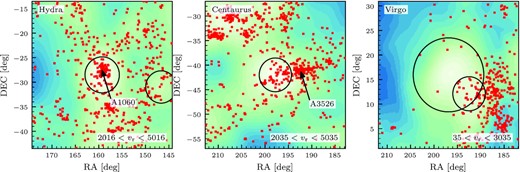
Fig. 10 shows the density field of galaxies surrounding the nine most massive haloes within the sibelius-dark volume. All galaxies within an RA and DEC of ±15 degrees and v_r ± 1500 km s⁻¹ of the sibelius-dark cluster centre are shown. Within the region, any sibelius-dark halo more massive than M_200c ≥ 10¹⁴ M_⊙ is shown as a black circle, with a radius of r_200c. Overplotted in red are galaxies from the 2M++ galaxy sample that cover the same volume, and we also indicate the location of the richest cluster from the Abell catalogue in the region. We then associate the most massive sibelius-dark halo that is closest to the Abell cluster location as the observational analogue. For seven of the nine haloes we are able unambiguously to associate an observed Abell cluster to their model haloes. In two cases, SD-C7_SD and SD-C8_SD, there is no Abell cluster in the region; yet there is a clear concentration of 2M++ galaxies in each case. We repeat this process for three famous lower mass clusters, Hydra, Centaurus, and Virgo in Fig. 11. Below, we examine how these sibelius-dark clusters compare to their observed counterparts. For many of the observed halo mass estimates we refer to those within the recent compilation of Stopyra et al. (2021) and references therein.

Figure 10.

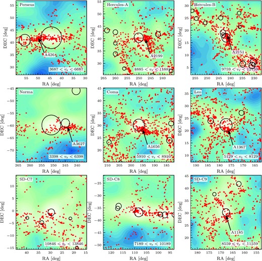
The large-scale structure surrounding the nine most massive haloes in the sibelius-dark volume. Each panel covers an RA and DEC of ±15 degrees and v_r ± 1500 km s⁻¹ surrounding the particular sibelius-dark halo. The contours in the background show the sibelius-dark galaxy density, increasing in logarithmic density from blue to green. Any sibelius-dark haloes more massive than M_200c ≥ 10¹⁴ M_⊙ are shown as black circles, with a radius of r_200c. Overplotted in red are galaxies from the 2M++ catalogue and, annotated with arrows, the location of the richest Abell cluster (Abell 1958; Abell, Corwin & Olowin 1989) in the region. There is no Abell cluster in the vicinity of SC-C7 and SC-C8, however there is a concentration of 2M++ galaxies at the location of the haloes. The properties of the nine clusters are listed in Table B1 and the properties of their most massive galaxies are listed in Table B2.

Figure 11.

As Fig. 10, now for the Centaurus, Hydra, and Virgo clusters.

Perseus: the Perseus-Pisces_* Supercluster is one of the most massive structures in the Local Universe, a long, dense wall of galaxies with a length of almost 100 Mpc (see Fig. 1). At one end of this wall lies the supercluster’s most dominant member, the Perseus_* cluster (A426), one of the most massive clusters observed within the local volume, and with a mass of M_200c = 2.72 × 10¹⁵ M_⊙, the most massive halo within sibelius-dark. There is considerable disagreement in the literature as to the mass of the Perseus_* cluster, ranging from a lower value of ≈9 × 10¹⁴ M_⊙ using X-ray data (Simionescu et al. 2011), to an upper value of ≈3 × 10¹⁵ M_⊙ from dynamical estimates (Meusinger et al. 2020). This puts Perseus_SD within the observed range, albeit towards the upper limit.

Hercules-A & Hercules-B: the Hercules_* Superclusters are a pairing of two superclusters connected over a large area of the northern sky: a northern supercluster, to whose richest member, A2199, we will refer to as Hercules-A_SD, and a southern supercluster, whose richest member is the Hercules_* cluster itself (A2151), to which we will refer as Hercules-B_SD. These two clusters, Hercules-A_SD and Hercules-B_SD, constitute the 2nd and 3rd most massive haloes in the sibelius-dark volume, with masses M_200c = 1.89 × 10¹⁵ M_⊙ and M_200c = 1.78 × 10¹⁵ M_⊙, respectively. Observationally, the mass estimates for Hercules-A_* are again uncertain, spanning almost a decade in mass from ≈2 × 10¹⁴ M_⊙ to ≈2 × 10¹⁵ M_⊙ between X-ray (Piffaretti et al. 2011), dynamical (Kopylova & Kopylov 2013; Lopes et al. 2018), SZ (Planck Collaboration XIII 2016b) and weak lensing (Kubo et al. 2009) estimators. The estimates for the mass of Hercules-A_* are likely complicated by the ongoing merger with its partner cluster, A2197 (Krempeć-Krygier, Krygier & Krywult 2002). For Hercules-B_*, the estimated mass range from the observations of (0.79–1.89) × 10¹⁵ M_⊙ (Lopes et al. 2018) is similar to Hercules-A_*. As with the supercluster of Hercules-A_*, the supercluster of Hercules-B_* is likely also dynamically bound and collapsing (Krempeć-Krygier et al. 2002; Kopylova & Kopylov 2013), which could significantly disrupt the resulting mass estimate. Compared to the sibelius-dark haloes, both Hercules-A_SD and Hercules-B_SD lie within the observed mass range, both towards the upper ends of the estimated ranges.

Norma: the Norma_* cluster lies extremely close to the galaxy’s ‘zone-of-avoidance’, where extinction is severe, and our understanding of the surrounding local large-scale structure remains incomplete. Norma_* is perhaps most famous for its connection to the ‘Great Attractor’, a region of the sky (shared by the Hydra, Centaurus, Norma and Shapley clusters) towards which many local galaxies, including the Local Group, are streaming en masse against the direction of the Hubble flow (Lynden-Bell et al. 1988). Due to its location, the mass of the Norma_* cluster, and its nature, remain poorly constrained, but is estimated to be in the range ≈3 × 10¹⁴ M_⊙ to ≈2 × 10¹⁵ M_⊙, with the upper end coming from dynamical estimates (Woudt et al. 2008). In sibelius-dark, Norma_SD is the 4th most massive halo, with a mass of M_200c = 1.72 × 10¹⁵ M_⊙, close to the observed dynamical mass estimates of the cluster.

Coma & Leo: the Coma_* Supercluster is one of the most famous and well-studied structures within the Local Universe. Located at a distance of approximately 100 Mpc, it consists of two primary members, the Coma_* Cluster (A1656) and the Leo_* Cluster (A1367), which are connected to one another via a rich network of filaments, in which a large number of groups and galaxies are embedded (e.g. Williams & Kerr 1981; Rines et al. 2001; Seth & Raychaudhury 2020). Coma_SD is the 5th most massive halo within the sibelius-dark volume, with a mass of M_200c = 1.27 × 10¹⁵ M_⊙, which lies within the range of observational estimates ≈3 × 10¹⁴ M_⊙ to ≈2 × 10¹⁵ M_⊙ (Kubo et al. 2009; Piffaretti et al. 2011; Planck Collaboration XIII 2016b). Leo_SD, the second primary member of the Coma_* Supercluster, is the 6th most massive halo in sibelius-dark directly behind Coma_SD, with a mass of M_200c = 1.17 × 10¹⁵ M_⊙. This makes Leo_SD noticeably more massive than the observational estimates (with an upper limit of ≈4 × 10¹⁴ M_⊙ from dynamical estimates; Rines et al. 2003). However, we note that Leo_* is observed to be a young, dynamically active system, with multiple ongoing mergers in the inner regions (Cortese et al. 2004), which could affect the mass estimates.

SD-C7 & SD-C8 & SD-C9: the 7th, 8th, and 9th most massive haloes within sibelius-dark have no commonly named counterpart in the data. Thus, we simply refer to them by their mass rank. Only SD-C9_SD has a counterpart in the Abell catalogue of clusters, A1185. Yet we note that SD-C7_SD and SD-C8_SD are clearly associated with a grouping of galaxies in the same location in the 2M++ catalogue.

Hydra & Centaurus: Hydra_* and Centaurus_* are a famous cluster pair in the southern sky, located in the foreground of Norma_*. The two clusters, A1060 and A3526, are less massive than the nine clusters discussed above, yet are thought to be major contributors to the structure of the Great Attractor (e.g. Raychaudhury 1989). In sibelius-dark, Hydra_SD is the 32nd most massive halo in the volume at M_200c = 4.9 × 10¹⁴ M_⊙, and Centaurus_SD is the 44th most massive, at M_200c = 4.1 × 10¹⁴ M_⊙. These masses are both well in line with observational estimates for the two clusters (∼10¹⁴ M_⊙; e.g. Richtler et al. 2011).

Virgo: the Virgo_* cluster, at a distance of ≈16 Mpc, is our most massive neighbour, a dynamically young and unrelaxed cluster with a relatively large number of substructures (Binggeli, Tammann & Sandage 1987). Our Virgo_SD Cluster, shown in the right-hand panel of Fig. 11, is located close to the observed location on the sky, yet is slightly too distant (≈21 Mpc). From the right-hand panel of Fig. 11, we see two haloes more massive than 10¹⁴ M_⊙ in the vicinity which, at first glance, would suggest an ongoing merger; however the smaller of the two haloes is approximately 15 Mpc behind Virgo_SD, and is not itself a member of the cluster. Virgo_SD is the 56th most massive halo in sibelius-dark, at M_200c = 3.5 × 10¹⁴ M_⊙, which is slightly below recent mass estimates for the cluster (≈5–7 × 10¹⁴ M_⊙; Shaya et al. 2017; Kashibadze, Karachentsev & Karachentseva 2020).

In this section, we have investigated twelve clusters on the sibelius-dark sky to see how well the constraints match the observations for particular objects. For each model cluster, we are encouraged that there is always a concentration of observed galaxies in close proximity, and the halo masses predicted by the simulation are often within the bounds of observational estimates. For all but two of these model haloes, SD-C7_SD and SD-C8_SD, we are able to associate a catalogued Abell cluster directly with them. This gives us confidence that these structures are reasonable analogues of the observed Universe, allowing us to make predictions as to their particular structure and formation. In the next section, we focus more closely on the particular structure of the Virgo_SD and Coma_SD clusters.

3.3 A closer look at the Virgo and Coma clusters

In the previous section, we established that the large-scale structure surrounding the most massive objects in the sibelius-dark volume matches well the observational data. Here we take the comparison one step further, by investigating the member galaxy populations of two of the local volume’s most famous occupants; Virgo and Coma. The analysis in Sections 3.3.1 and 3.3.2 are deliberately brief, as we reserve a more in depth comparison to the properties and evolution of particular structures to future work. Our goal here is to reassure the reader that sibelius-dark produces reasonable analogues to observed clusters, giving confidence to then go on and use these analogues to make predictions as to a plausible nature and evolution. One such example prediction is presented in Section 3.3.3, where we investigate the location and observability of the ‘splashback radius’ for the two clusters. We remind the reader however, that as sibelius-dark is built upon a single borg realization, one designed to reproduce the local volume en masse, we caution against overinterpreting the exact nature of individual structures.

3.3.1 Observing the Virgo cluster

The Virgo cluster remains to this day one of the most well-studied objects within our Universe; at relatively close proximity (≈16 Mpc; Blakeslee et al. 2009), with such a large mass (≈5 × 10¹⁴ M_⊙; Kashibadze et al. 2020), Virgo is a prime target for studying cluster environments. Indeed, the Virgo cluster has long been a testbed for the luminosity function in cluster environments, with results often being revised as deeper and more complete data becomes available, particularly for the prediction of the faint-end slope (α ≈ −1 → −2, e.g. Binggeli, Sandage & Tammann 1985; Sandage, Binggeli & Tammann 1985; Impey, Bothun & Malin 1988; Rines & Geller 2008).

The Next Generation Virgo Cluster Survey (NGVCS; Ferrarese et al. 2012) is the deepest and most complete optical survey of the Virgo cluster’s core region (the innermost ≈3.7 deg²), down to a point-source depth of g ≈ 25.7 mag. In Fig. 12 we show the distributions of stellar mass and absolute g-band magnitude for the galaxies in the NGVCS survey (Ferrarese et al. 2016). As the data have already been corrected to remove foreground and background interlopers, we compare against the distributions of sibelius-dark galaxies within a r = 0.2 Mpc spherical aperture centred on the sibelius-dark M87 analogue, which approximately equates to the surveyed area. The match between the sibelius-dark Virgo analogue and the data is extremely encouraging; the magnitude gap of ≈1 between M87 and the next brightest member is reproduced, the overall number of bright galaxies in the cluster is consistent, and the slope and normalization of the faint end agree well. Considering also the stellar mass in the upper panel, we again find a good agreement between the two data sets.

Figure 12.

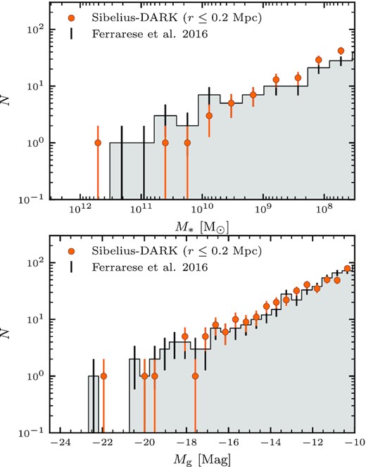
The galaxies within the core (r = 0.2 Mpc) of the sibelius-dark Virgo cluster (orange points); distributed by stellar mass (upper panel) and g-band absolute magnitude (lower panel). We compare against observational data from the Next Generation Virgo Cluster Survey (grey histograms and black errorbars; Ferrarese et al. 2016). Poisson errors are shown in both cases. There is a good agreement between the member population of the model sibelius-dark Virgo cluster and the data.

At the centre of the Virgo cluster lies M87, its central elliptical galaxy. The sibelius-dark analogue for M87 has a stellar bulge mass of M_{*, bulge} = 3.6 × 10¹¹ M_⊙ and hosts a supermassive black hole of mass M_BH = 3.2 × 10⁹ M_⊙. Compared to the compilation data from Sahu et al. (2019) (plotted in Fig. 6), with observed masses of M_{*, bulge} = (1.7–5.6) × 10¹¹ M_⊙ and M_BH = (5.2–6.3) × 10⁹ M_⊙, this puts the sibelius-dark analogue for M87 well within a factor of 2 for both properties.

3.3.2 Observing the Coma cluster

The Coma cluster is more massive (>10¹⁵ M_⊙) and more distant (≈100 Mpc) than Virgo, which makes identifying cluster members much more challenging, and requires robust spectroscopic redshifts to reduce contamination by foreground and background objects. Applying the caustic technique is a popular observational method to identify cluster members using spectroscopic samples (Diaferio & Geller 1997).

In the upper panel of Fig. 13, we examine the observed galaxies from SDSS DR12 data that surround the Coma cluster, showing the rest-frame cluster-centric radial velocity versus projected cluster-centric distance. The values for the radial velocity and position of the observed Coma cluster (i.e. the reference frame) are taken from Sohn et al. (2017), and only galaxies within the spectroscopic completeness limit of SDSS, r < 17.77, are considered. Cluster members are identified as those that fall within the outlined caustic, which has been computed by Sohn et al. (2017) using the same SDSS data. Also shown are the sibelius-dark Coma member galaxies, with both properties now computed from the reference frame of the sibelius-dark Coma BCG (detailed in Table B2). We use the same caustic outline to identify the member galaxies of the sibelius-dark Coma cluster.

Figure 13.

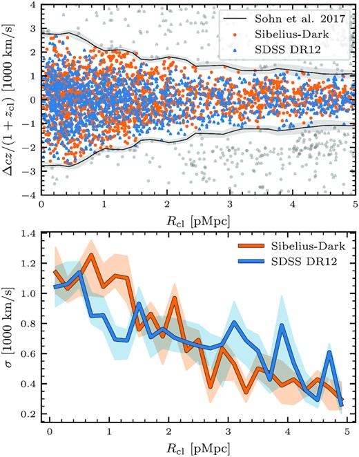
Top: rest-frame cluster-centric radial velocity versus projected cluster-centric distance for SDSS (blue) and sibelius-dark (orange) galaxies surrounding their respective Coma clusters. Member galaxies are those that fall within the caustic outlines (grey), computed by Sohn et al. (2017) using SDSS data. Bottom: velocity dispersion of member galaxies within each projected radial bin. Errors are from bootstrap resampling.

By eye, in the upper panel of Fig. 13, there is overall good agreement between the model and observed populations. To examine the comparison more closely, the bottom panel of Fig. 13 shows the one-sigma dispersion of velocities within each projected radial bin. The errors here are computed by bootstrap resampling the velocities within each projected radial bin, showing the 10th to 90th percentile range of the resulting dispersion. The trends for the model and observed Coma cluster are encouragingly similar; the dispersion of velocities decreases with increasing distance from the cluster centre, as one would expect, from ≈1100 km s⁻¹ at the cluster core, to ≈650 km s⁻¹ at 2.25 projected Mpc (the approximate location of the observed virial radius for Coma, Sohn et al. 2017), with the only disparity coming at ≈1 projected Mpc, where the sibelius-dark Coma cluster has a higher dispersion.

At the centre of the Coma cluster lies NGC 4889, its brightest galaxy. The sibelius-dark analogue for NGC 4889 has a stellar bulge mass of M_{*, bulge} = 8.6 × 10¹¹ M_⊙ and hosts a supermassive black hole of mass M_BH = 5.3 × 10⁹ M_⊙. Compared to the compilation data from Sahu et al. (2019) (plotted in Fig. 6), with observed masses of M_{*, bulge} = (0.9–1.7) × 10¹² M_⊙ and M_BH = (0.6–3.7) × 10¹⁰ M_⊙, this puts the sibelius-dark analogue right at the lower mass estimate for both the galaxy and the central black hole. However, it is worth noting that NGC 4889 hosts one of the most massive black holes ever discovered in the nearby Universe, lying far above the predicted black hole mass for the mass of the stellar bulge (McConnell et al. 2011), which would be challenging for any model of galaxy formation to reproduce exactly.

The results from Figs 12 and 13 have given us confidence that the clusters in sibelius-dark are reasonable analogues of the observational counterparts, which we can then go on and use to make predictions.

3.3.3 A theoretical prediction for the ‘Splashback Radius’ of Virgo and Coma

In recent years an increasing amount of attention has been focused on the ‘splashback radius’ of dark matter haloes, a caustic formed from the ‘bunching up’ of mass elements that have just reached the apocentre of their first orbits (e.g, Adhikari, Dalal & Chamberlain 2014). The physical signature of this effect is seen as a sudden drop in the outer regions of the density profile (e.g. Diemer & Kravtsov 2014), creating a divergence from the universal analytic profiles discussed in the literature, such as the Navarro–Frenk–White (NFW; Navarro, Frenk & White 1996, 1997) and Einasto profiles (Navarro et al. 2010). It is suggested that the splashback radius provides a more intuitive metric to define the size of a dark matter halo, and avoids the shortcomings of more arbitrary definitions of halo extent which are coupled to the expansion of the Universe, such as those based on a chosen density contrast (e.g. Diemer, More & Kravtsov 2013). To recover the splashback radius one requires an adequate tracer of the underlying density profile within the halo, from either the dark matter or stellar distribution, or the subhalo population. The splashback radius can additionally be recovered in velocity space from the same tracers. We note that whilst sibelius-dark is a DMO simulation, it has been shown that the inclusion of hydrodynamics has almost no effect on the location of the splashback radius (e.g. Contigiani, Bahé & Hoekstra 2021; O’Neil et al. 2021).

Figs 14 and 15 show, respectively, Virgo and Coma’s cluster-centric dark matter density and radial velocity profiles. As is common in this field, we scale the radii by r_200m, i.e. the radius at which the haloes enclosed mass reaches 200 times the mean density (200Ω_mρ_crit), and the radial velocities by |$v_{\mathrm{200m}} = \sqrt{G M_{\mathrm{200m}} / r_{\mathrm{200m}}}$|⁠, i.e. the circular velocity at r_200m. We compute the profiles in 40 equally spaced logarithmic bins of r/r_200m in the range ∈ [−1, 0.6], and in ten azimuthal bins of 36 degrees centred on the clusters potential minimum. The profiles presented are the median density/velocity in each radial bin between the multiple sightlines, a process designed to minimize the underlying bias from interloping massive substructures within the halo in a particular direction⁸ (e.g. Mansfield, Kravtsov & Diemer 2017; Deason et al. 2020). We estimate the error on the median value by bootstrap resampling the multiple sightlines, indicated by the shaded regions, and we then apply a fourth-order smoothing algorithm (Savitzky & Golay 1964) to the median profiles in order to better recover the features. Finally, we compute the gradient of the median lines in the upper panels using linear regression, fitting the slope of the median lines in intervals of five bins using SciPy’s curve_fit function (Virtanen et al. 2020). This gradient is then shown in the lower panels. The splashback radius, r_sp, is identified as the sudden dip in these gradients, seen at approximately the virial radius.

Figure 14.

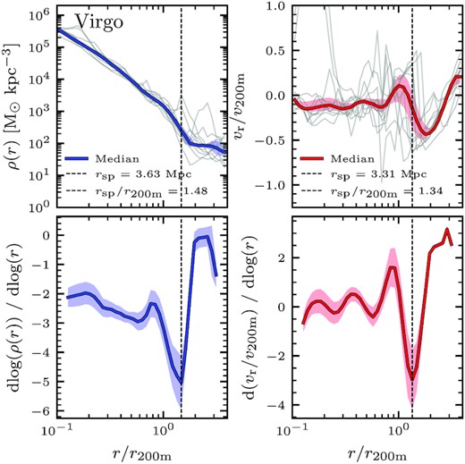
Top: the density (left-hand panel) and radial velocity (right-hand panel) profiles of the dark matter particles measured from the Virgo clusters potential centre. Individual grey lines show the profiles measured within 10 arbitrary bins of azimuthal angle, with the solid coloured lines representing the median density/velocity within each radial bin between the 10 sightlines. The error on the median, shown as a shaded region, is computed via bootstrap resampling. Bottom: the logarithmic slopes of the above profiles. Here we can clearly identify the characteristic change in gradient at the outer edges of the halo relating to the ‘splashback radius’, r_sp, measured to be 3.63 ± 0.34 Mpc and 3.31 ± 0.31 Mpc from the density and velocity profiles, respectively. The quoted errors for r_sp are the bin width.

Figure 15.

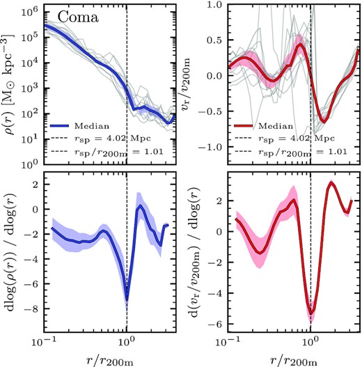
As Fig. 14, now for the Coma cluster. The ‘splashback radius’ for the Coma cluster is measured to be 4.02 ± 0.38 Mpc from both the density and velocity profiles.

For both the Virgo and Coma clusters, the density and velocity profiles in Figs 14 and 15 each show a clear primary caustic in the lower panels at ≈r_200m. It is worth noting that both haloes additionally show tentative evidence for a secondary caustic within r_200m, which is theoretically linked to the second apocentre passage of material within the halo (a feature which becomes more prominent for haloes at lower accretion rates, e.g. Adhikari et al. 2014). However, given that here we are only considering the profiles of individual haloes, whose results can be particularly sensitive to recent/ongoing mergers or asymmetrical accretion, we choose not to overinterpret the trends, and only concentrate on the primary caustic at the splashback radius.

The splashback radius of Virgo is r_sp = 3.63 ± 0.34 Mpc and that of Coma is 4.02 ± 0.38 Mpc measured from the density profile and r_sp = 3.31 ± 0.31 Mpc and 4.02 ± 0.38 Mpc measured from the velocity profile. Or, when scaled by r_200m, they are equivalently r_sp/r_200m = 1.48 ± 0.14 and 1.01 ± 0.09 measured from the density profile and r_sp/r_200m = 1.34 ± 0.12 and 1.01 ± 0.09 measured from the velocity profile for Virgo and Coma respectively. The quoted errors are the bin width. Many factors have an impact on the location of the splashback radius for a given halo; its mass, the cosmology, the redshift, and perhaps most importantly, the halo accretion rate,

$$\begin{eqnarray*} \Gamma _{\mathrm{0.5}} = \frac{\Delta \mathrm{log} M_{\mathrm{200m}}}{\Delta \mathrm{log}(1+z)}, \end{eqnarray*}$$

(2)

computed in the range z = 0.5 to z = 0 (Diemer & Kravtsov 2014; More, Diemer & Kravtsov 2015; Diemer et al. 2017). In sibelius-dark, the Coma cluster has a smaller value of r_sp/r_200m both because it is more massive, and because it has a higher accretion rate (Γ_0.5[Coma] = 5.4 versus Γ_0.5[Virgo] = 1.5). We note that the measured values for r_sp/r_200m are consistent with the theoretical trends for the general population of dark matter haloes (More et al. 2015; Diemer et al. 2017; Contigiani et al. 2021).

Until now we have been considering the density and radial velocity profiles of Virgo and Coma using the abundance of dark matter particles. Yet, the location of the splashback feature can also be retrieved using the subhalo population of the cluster. Fig. 16 repeats the analysis of the right-hand panels of Figs 14 and 15, now using the cluster-centric radial velocities and distances of the subhalo members with stellar masses M_* ≥ 10⁸ M_⊙. Due to the reduced numbers involved in this method, we no longer average the profiles over multiple azimuthal bins, and instead consider complete radial shells. The errors on the median are computed by bootstrap resampling the subhaloes within each radial bin, and the gradients in the lower panels are computed in the same way as for Figs 14 and 15. Once again the primary caustic of the splashback radius is robustly detected, yet now at values ≈10 per cent lower than was found when directly using the dark matter particles. This is consistent with previous simulation studies, which argue that the increased dynamical friction felt by the subhalo members may be the cause for the smaller radii (Xhakaj et al. 2020).

Figure 16.

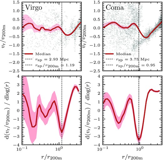
A repeat of the analysis from the right-hand panels of Figs 14 and 15, now using the cluster-centric radial velocities and distances of the galaxies, rather than the dark matter particles. The grey points mark individual galaxies with stellar masses M_* ≥ 10⁸ M_⊙, and the solid lines represent the smoothed medians. We again find the primary caustic of the splashback feature, at 2.92 ± 0.32 Mpc and 3.75 ± 0.41 Mpc for the Virgo and Coma clusters, respectively. These values are ≈10 per cent lower than the radii found when directly using the dark matter particles.

We conclude this section with a brief observational experiment. The splashback feature has been detected observationally in galaxy clusters by stacking the data over many sources, either using the luminosity density profiles of the galaxy members (e.g. More et al. 2016; Baxter et al. 2017; Nishizawa et al. 2018; Murata et al. 2020; Bianconi et al. 2021) or via weak gravitational lensing (Contigiani, Hoekstra & Bahé 2019). The feature has also tentatively been observed in the intracluster light of individual clusters (e.g. Gonzalez et al. 2021). Here we consider a similar approach, investigating if the splashback radius of the sibelius-dark Virgo cluster can be recovered using the line-of-sight velocities of the member galaxy population.

We select the galaxies with stellar masses greater than M_* ≥ 10⁸ M_⊙ within 3 × r_200m of the sibelius-dark Virgo cluster. The cluster-centric distances and cluster-centric radial velocities of the Virgo members are computed ‘observationally’; using their distance from the Milky Way (d_MW), their line-of-sight velocity (v_r) and their angular position relative to the Virgo BCG using the transformations of Karachentsev & Kashibadze (2006) (see also the Appendix of Sorce et al. 2021). When considering distance errors to the Virgo member galaxies in the analysis below, we add a random scatter to the Milky Way distance (Δd_MW) drawn from a uniform distribution of the quoted magnitude before computing the cluster-centric properties. We assume no errors on the line-of-sight velocities of the cluster members or their positions on the sky, and we add no distance error to the Virgo BCG (i.e. our central reference point for the cluster).

We present the results in Fig. 17. The upper panel is a repeat of the lower left-hand panel from Fig. 16, i.e. the gradient of the slope of the cluster-centric radial velocities for Virgo galaxies (blue line), computed using the full 3D velocity information, with the characteristic dip at r_sp/r₂₀₀ = 1.19 being the splashback radius as seen previously. In orange is the equivalent measurement, but now we have estimated the cluster-centric radial velocities using the 1D line-of-sight velocities as viewed from the Milky Way. In both cases we have not included an error on the galaxy distance from the Milky Way (Δd_MW = 0). From this we can already see that the loss of velocity information (i.e. 3D → 1D) serves to reduce the prominence of the splashback feature, yet it does not change its location.

Figure 17.

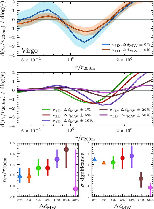
‘Observing’ the splashback radius of the Virgo cluster using member galaxies above M_* ≥ 10⁸ M_⊙. The top panel is a repeat of the lower left-hand panel of Fig. 16, i.e. the gradient of the cluster-centric radial velocities, using 3D and 1D (line-of-sight velocity) velocity information. Simply going from 3D to 1D velocities already serves to reduce the prominence of the dip in the splashback feature. In the middle panel, we now include random Milky Way distance errors to each galaxy sampled from a uniform distribution of the quoted magnitude. For each value of the distance error, we perform the experiment 100 times, with each line in the middle panel showing the median value of d(v_r/v_200m)/dlog(r) between the 100 measurements. No errors (shaded regions) are shown in this panel for clarity, yet they are comparable to those in the panel above. As the distance error increases, so to does the location of the splashback feature (shown in the lower left-hand panel). Additionally, as the distance error increases above 10 per cent, the splashback feature is no longer significantly detected (lower right-hand panel). We define the significance (σ) to be the ratio of the value of the splashback feature below zero divided by the error. The values in the lower panels are the median values between the 100 measurements, and the errors are the 10th to 90th percentile range (or for just the lower left-hand panel, at least the bin width).

In the middle panel of Fig. 17 we now include random errors on the distance from the Milky Way to the Virgo member galaxies (Δd_MW), to investigate how this influences the location of the splashback radius. To do this we sample a random distance error for each galaxy from a uniform distribution of the quoted magnitude, compute d(v_r/v_200m)/dlog(r) for this new realization, and retrieve the location of r_sp/r_200m. We then repeat this experiment 100 times for each magnitude of the distance error, with the lines in the middle panel showing the median values of d(v_r/v_200m)/dlog(r) between the 100 realizations. The median location of r_sp/r_200m between the 100 realizations as a function of the distance error is shown in the lower left-hand panel, including also the location of the splashback feature without any distance errors (i.e. the values from the upper panel). The errorbars represent the uncertainty, which is the maximum value between the bin width and the 10th to 90th percentile range between the 100 realizations (when applicable). We define the ‘significance’ (σ) of the feature as the ratio between the absolute value of d(v_r/v_200m)/dlog(r) divided by the width of the error on d(v_r/v_200m)/dlog(r). The lower right-hand panel shows the median value of σ as a function of distance error between the 100 realizations (the errorbars represent the 10th to 90th percentile range).

We find that as the distance error increases, the location of the splashback feature also increases to higher radii, from r_sp/r₂₀₀ ≈ 1.3 at Δd_MW = 1 per cent to r_sp/r₂₀₀ ≈ 1.5 at Δd_MW = 10 per cent. The significance of the dip is also dependent on the distance error, with distance errors below 10 per cent remaining detectable with a significance on average above 3σ, yet when the distance errors increase above 10 per cent the feature is essentially lost. We then predict that only with a complete census of the Virgo cluster member galaxies above M_* ≥ 10⁸ M_⊙, with distance errors Δd_MW ≤ 10 per cent, can the splashback feature be recovered.

3.4 The Local Group and the local neighbourhood

At approximately the centre of the sibelius-dark volume lies a dark-matter halo pair that matches closely the observed dynamics of our own Local Group’s Milky Way and Andromeda haloes, a deliberate result of the embedment procedure that created the constrained initial condition set (see Section 2.1.1). All the properties detailed below are also listed in Table B3. The model Milky Way and Andromeda have halo masses M₂₀₀ = 0.9 × 10¹² M_⊙ and M₂₀₀ = 1.3 × 10¹² M_⊙, respectively, matching well the current observational estimates (∼10¹² M_⊙, i.e. Watkins, Evans & An 2010; Posti & Helmi 2019; Cautun et al. 2020). Viewed from the model Milky Way, the model Andromeda galaxy is at a distance of 753 kpc, putting it well within the observed range (752 ± 27 kpc, Riess, Fliri & Valls-Gabaud 2012); has an infalling radial velocity of −117 km s⁻¹, very close to the observed value (−109.3 ± 4.4 km s⁻¹; van der Marel et al. 2019) and has a low tangential velocity, 33 km s⁻¹, also well in line with observational constraints (⁠|$56^{+35}_{-31}$| km s⁻¹ from Gaia DR2 and HST data and 164.4 ± 61.8 km s⁻¹ from satellite kinematics, Salomon et al. 2016; van der Marel et al. 2019).

It is encouraging, yet unsurprising, that the halo masses and dynamics of the model Local Group match so well the observations, as they were deliberately designed to be so. As a reminder, the exploration runs of Sawala et al. (2022) used to generate the eventual initial conditions of sibelius-dark were dark-matter-only, and thus we were unable to consider the galaxy/baryonic properties of the Local Group candidates during the process. There was no guarantee therefore that the model properties of the Milky Way and Andromeda predicted by the semi-analytic model would turn out correct. Indeed, the total stellar mass for the model Milky Way, at M_* = 5.43 × 10⁹ M_⊙, is approximately an order of magnitude too low compared to the estimated value of M_* = (4–7) × 10¹⁰ M_⊙ (e.g. Licquia & Newman 2015), and the model Andromeda total stellar mass, at M_* = 6.38 × 10⁹ M_⊙, is similarly an ≈order of magnitude too low compared to the estimated value of M_* = (7–15) × 10¹⁰ M_⊙ (e.g. Tamm et al. 2012; Rahmani, Lianou & Barmby 2016). These are, of course, sensitive to the particular choice of semi-analytic galaxy formation model chosen, and also could change considerably if a full hydrodynamical simulation was performed on the same initial condition set. Additionally, the halo masses of the Milky Way and Andromeda lie at a critical juncture for galaxy formation physics, right at the onset of the AGN feedback regime (Bower et al. 2012; McAlpine et al. 2018), which results in a large spread of stellar masses for a given halo mass, particularly for the galform model (see fig. 4 of Guo et al. 2016). Regardless, for future generations of the sibelius project we will consider also the baryonic properties during the exploration process, in order to further improve the Local Group analogues.

3.4.1 The ‘bulk flow’ of the local neighbourhood

We now investigate what immediately surrounds the model Local Group pair, what we dub the ‘Local Neighbourhood’. Fig. 18 shows the projected dark matter distribution in a (50 Mpc)³, (15 Mpc)³, and (5 Mpc)³ volume centred on the model Milky Way. We find that the Local Group pair reside within a relatively isolated filament, and are eventually bracketed almost symmetrically by the Fornax and Virgo clusters at larger scales.

Figure 18.

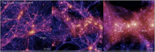
The left-hand panel shows the dark matter distribution in a 50×50×50 Mpc region centred on the Milky Way, coloured by the projected density and velocity dispersion of the particles. Our two most massive neighbours, the Virgo cluster and the Fornax/Eridanus groups, are highlighted. The middle and right-hand panels zoom into a 15×15×15 Mpc and 5×5×5 Mpc region, respectively. The right-hand panel highlights the location of the Milky Way and Andromeda (M31). Images are shown in y–z equatorial coordinates, projected down the x axis.

An interesting observed feature relating to the nature of the Local Neighbourhood, and beyond, is the existence of the ‘bulk flow’; a coherent motion of galaxies in the vicinity of the Local Group towards a common location, against the direction of the Hubble flow. This common location is often referred to as the ‘Great Attractor’ (Lynden-Bell et al. 1988), and it is located in the approximate direction of the Hydra and Centaurus clusters.

To investigate the motion of sibelius-dark galaxies in the Local Neighbourhood we present Fig. 19. This shows, for all central galaxies within 10 Mpc of the Milky Way with a stellar mass greater than M_* > 10⁷ M_⊙, the direction of the peculiar velocity vector in the CMB reference frame with-respect-to the location of the sibelius-dark Hydra cluster. That is, using an absolute set of coordinate axes (the conventional Galactic coordinate axes), we locate the observed position of the Hydra cluster on the sky from the reference frame of each galaxy and compare that position vector to the CMB reference frame velocity vector for that galaxy. Or, put another way, we ask when viewed from each galaxy, ‘how closely am I moving towards the simulated Hydra cluster?’.

Figure 19.

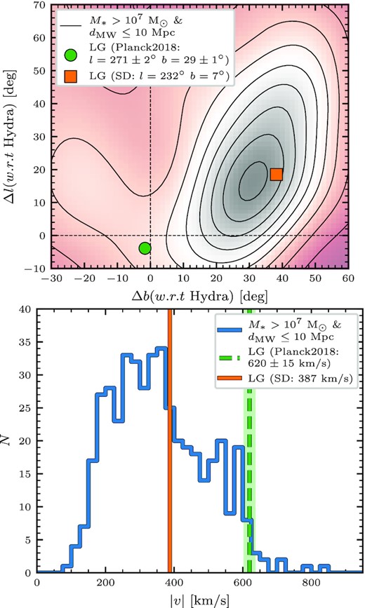
Top: direction of the velocity vectors in the CMB reference frame for central galaxies with mass M_* ≥ 10⁷ M_⊙ within a distance of 10 Mpc from the Milky Way. The velocity vectors are shown with respect to the location of the sibelius-dark Hydra cluster on the sky, as viewed from each galaxy’s reference frame, using the galactic coordinate system (l, b). The observed direction of the Local Group’s motion points very close to the Hydra cluster (Planck Collaboration VI 2020), whereas the sibelius-dark Local Groups’s motion, and that of the majority of galaxies surrounding the sibelius-dark Local Group, points Δl ≈ +20° and Δb ≈ +30° relative to the Hydra cluster. Bottom: magnitude of the velocity for each galaxy in the CMB reference frame. The sibelius-dark Local Group has a peculiar velocity ≈225 km s⁻¹ less than the observed value (Planck Collaboration VI 2020).

From the upper panel of Fig. 19, we find that the majority of galaxies in the region of the Local Neighbourhood (including the Local Group) are flowing in a communal direction, approximately +30 degrees in Galactic longitude and +20 degrees in Galactic latitude with-respect-to the position of the Hydra cluster. From Fig. 1, this points somewhere between the Virgo and Centaurus clusters in the Northern hemisphere. Compared to the observed direction of the Local Group’s motion, computed from the CMB dipole (Planck Collaboration VI 2020), this is off by approximately the same amount, as the observed vector of motion points almost exactly at the location of the sibelius-dark Hydra cluster. In the lower panel, we show the distribution of magnitudes for the velocity vectors of these galaxies. As with the direction, the Local Group is ‘typical’ compared to the galaxies surrounding it, with an absolute velocity of 387 km s⁻¹. This is ≈225 km s⁻¹ below the observed value (620 ± 15 km s⁻¹; Planck Collaboration VI 2020). It is extremely challenging to state where this discrepancy stems from, given how sensitive this result can be to the particular structural distribution surrounding the Local Group. One example could be the location of the sibelius-dark Virgo cluster, which is ≈40 per cent more distant than the observed Virgo cluster. Also, it has been argued that many objects contribute to the Local Group’s bulk flow, including Hydra, Centaurus, Norma and even as far as Shapley, which all reside in a communal area on the sky at ever increasing distances. It is possible therefore that structures beyond our constraints (d_mw > 200 Mpc) would provide the remaining contribution to the bulk flow (e.g. Turnbull et al. 2012; Boruah, Hudson & Lavaux 2020), however it is perhaps unlikely that structures beyond 200 Mpc could make up for such a discrepancy. It would take a detailed study beyond the scope of this work to fully establish the origin of this discrepancy, however it will be an important consideration for improving future generations of sibelius constrained initial conditions.

4 DISCUSSION AND CONCLUSIONS

Whilst this study has largely been a presentation of the sibelius-dark simulation, in which here we have investigated the accuracy of the constrained initial conditions at z = 0 and provided examples of how to select specific structures and associate them with observational counterparts, it has also yielded interesting results relating to our local volume’s ‘unusual’ nature. We discuss two aspects here: (1) the number of haloes within the local volume with masses above |$M_{\mathrm{200c}} \ge 10^{15}\, h^{-1}$| M_⊙ and (2) the underdensity of the local volume within d_MW ≤ 200 Mpc (or ‘Local Hole’).

4.1 The number of haloes more massive than |$M_{\text{200c}} \ge 10^{15}\, h^{-1}$| M_⊙ in the local volume

First, we investigate the prevalence of the most massive haloes within the local volume, i.e. those with halo masses, |$M_{\mathrm{200c}} \ge 10^{15}\, h^{-1}$| M_⊙. Given the theoretical predicted exponential cutoff at the high-mass end of the halo mass function, a few, or even a single unexpected halo at these masses can pose a significant challenge to the underlying theory (Frenk et al. 1990). Here, we compare the predictions of sibelius-dark to the recent study by Stopyra et al. (2021), who attempt to quantify the rarity of the local volume by comparing the number of observed haloes above the |$\ge 10^{15}\, h^{-1}$| M_⊙ threshold to that predicted by a ΛCDM simulation. By analysing the halo mass function from the Horizon Run 4 ΛCDM simulation (Kim et al. 2015), Stopyra et al. (2021) predict an expectation value of |$\mathcal {O}(1)$| supermassive clusters per local volume. The likelihood of finding N clusters greater than M_200c ≥ 10¹⁵h⁻¹ M_⊙ in ΛCDM then follows a Poisson distribution,

$$\begin{eqnarray*} \mathcal {L}(N|N_{\mathrm{exp}}) = \frac{N_{\mathrm{exp}}^{N} e^{-N_{\mathrm{exp}}}}{N!}, \end{eqnarray*}$$

(3)

where N_exp = 1 as mentioned above.

Ultimately, Stopyra et al. (2021) are unable to conclusively estimate the local volume’s rarity in this respect, as the uncertainties in the halo mass estimators from observations are simply too large, giving a range of values of N between 0 and 5. For sibelius-dark, we find N = 4 haloes more massive than M_200c ≥ 10¹⁵h⁻¹ M_⊙: Perseus, Hercules-A, Hercules-B, and Norma (see Table B1). Stopyra et al. (2021) theoretically predict the likelihood of finding so many massive clusters in something the size of the local volume (i.e. the volume of sibelius-dark) to be 1.3 × 10⁻², which could certainly be classed as ‘rare’. We note, however, that this interpretation is reliant on a reasonable estimate of the original expectation value. Also, we accept that sibelius-dark is a single realization of the borg Markov chain, and, as the numbers here are so small, investigating N for multiple realizations would give a clearer picture as to the predicted number of supermassive haloes from sibelius. Yet, from sibelius-dark, we predict that there is potentially an abnormally large number of supermassive clusters occupying the local volume.

4.2 The underdensity of the local volume, a ‘Local Hole’?

Knowing if we reside in a particularly unusual region of the Universe, say a large underdensity, can be crucial for interpreting the results from local observations. One particular point of interest is in relation to the measurement of H₀, where an unusually large underdensity at the position of the observer would serve to increase the inferred expansion rate, which, if true, would alleviate some of the tension between the local (Riess et al. 2016) and Cosmic Microwave Background (CMB) measurements (Planck Collaboration XIII 2016a) of H₀. Many studies have argued for the existence of such a large-scale void, potentially stretching as far out as 150–200h⁻¹ Mpc, quoting the local volume to be underdense by up to values of ≈30 per cent (Zehavi et al. 1998; Whitbourn & Shanks 2014, 2016; Hoscheit & Barger 2018; Böhringer, Chon & Collins 2020). Critiques against many of these studies point to the assumption of isotropy when extrapolating results from a subset of the sky to the entire volume. However, an underdensity of 20 per cent has recently been proposed through a similar analysis using consistent all-sky data (Wong et al. 2021). Whilst underdensities at these levels could alter the reported value of H₀ by as much as ≈5 per cent, the scale of such an underdensity in a volume so large is almost impossible in ΛCDM (Wu & Huterer 2017).

Wong et al. (2021) find the n(z) and n(m) counts from the 2M++ survey to be ≈20 per cent lower than the homogeneous model of Whitbourn & Shanks (2014), which would imply an underdensity at the same level within z < 0.05. In Fig. 7 we investigated the same n(z) and n(m) distributions for sibelius-dark galaxies with K < 11.5, and compared to the data of the 2M++ survey. Given the agreement between sibelius-dark and the 2M++ data, it is safe to assume that an analysis similar to Wong et al. (2021) applied to the simulation data would yield a similar underdensity estimate relative to the homogeneous model of Whitbourn & Shanks (2014). However, in the simulation we have the advantage of being able to measure the density of the volume directly, which was reported in Fig. 4. We found the volume to be 5 per cent underdense at the boundary of the constraints (d_MW = 200 Mpc, or z ≈ 0.045), a 2σ deviation in ΛCDM (a result that is unlikely to change much for different choices of borg Markov chain, see Jasche & Lavaux 2019). Therefore we would argue that an exceptional deviation from ΛCDM, in terms of a large-scale underdensity, is not required to reproduce the observed number counts of galaxies in the local volume.

In this work we have presented sibelius-dark, a dark-matter-only (DMO) simulation paired with the semi-analytic model galform that uses the sibelius constrained initial conditions to replicate the density and velocity field of the local volume out to a distance, d_MW ≤ 200 Mpc, from the Milky Way. Overall, sibelius-dark provides the most comprehensive constrained realization simulation to date. The local volume’s large scale structure is replicated en masse with high fidelity (see Fig. 1 and the borg results from Jasche & Lavaux 2019). Statistically, the galaxies that populate sibelius-dark reproduce well the observed stellar mass distribution, luminosity distributions, central supermassive black hole population (see Figs 6 and 5) and number counts (see Figs 7 and 9) in the local volume.

Specific structures are generally present in the correct location of the sky and at the correct distance from the Milky Way (such as the Perseus, Hercules, Norma, Coma, Leo, Hydra, Centaurus, and Virgo clusters; see Figs 10 and 11 and reference Table B1 and Table B2), which provides a realistic spatial galaxy distribution (see Fig. 2). When these clusters are probed more closely, they represent well their counterparts in the observations (judged, for example, by the luminosity function of the cluster members; see Fig. 12), which can then be used to make predictions that are currently beyond our observational capabilities (for example, the location of the ‘splashback radius’ of local clusters, see Fig. 14). Finally, at the centre of the volume, sibelius-dark contains a halo pair that closely resembles the observed dynamics of the Local Group (see Section 3.4).

sibelius-dark is the first production simulation of the sibelius project (Sawala et al. 2022), demonstrating the potential of data sets from large-scale constrained realization simulations using the sibelius initial conditions. Some of the next stages of research for the sibelius project include: (1) resimulating the sibelius volume with full hydrodynamics, (2) resimulating multiple realizations of the borg constraints to estimate the variance in the formation histories and final-day properties of massive clusters within the local volume and (3) refining the reconstruction processes that produce the initial conditions, allowing for more accurate and extensive constraints in the next generation of sibelius simulations.

With the publication of this study, we publicly release the halo and galaxy catalogues of sibelius-dark at z = 0. See Section  A for details of how to access the catalogue and caveats of which to be aware when comparing to observational data.

ACKNOWLEDGEMENTS

The authors would like to thank the referee for their suggestions that have improved the quality of this work. We also thank Alastair Basden, Peter Draper, and the COSMA support team for their technical expertise that made this simulation possible. SM thanks Tom Shanks and Jonathan Wong for their helpful conversations, and particularly Ruari Mackenzie for his assistance with many observational data sets.

The simulation in this paper made use of the swift open-source simulation code (www.swiftsim.com, Schaller et al. 2018) version 0.9.0.

This work was supported by the Academy of Finland: grant numbers 314238 and 335607. PHJ acknowledges the support by the European Research Council via ERC Consolidator Grant KETJU (no. 818930). MS is supported by the Netherlands Organisation for Scientific Research (NWO) through VENI grant 639.041.749. CSF acknowledges support by the European Research Council (ERC) through Advanced Investigator DMIDAS (GA 786910). GL acknowledges financial support by the French National Research Agency for the project BIG4, under reference ANR-16-CE23-0002, and MMUniverse, under reference ANR-19-CE31-0020.

This work used the DiRAC Data Centric system at Durham University, operated by the Institute for Computational Cosmology on behalf of the STFC DiRAC HPC Facility (www.dirac.ac.uk). This equipment was funded by BIS National E-infrastructure capital grant ST/K00042X/1, STFC capital grants ST/H008519/1, and ST/K00087X/1, STFC DiRAC Operations grant ST/K003267/1 and Durham University. DiRAC is part of the National E-Infrastructure.

This work has been done within the Aquila Consortium (https://www.aquila-consortium.org).

DATA AVAILABILITY

We make public the halo and galaxy catalogues of the sibelius-dark simulation at z = 0 (see Section  A). The particle data for the simulation is available upon reasonable request.

Footnotes

1

The 2M++ galaxy sample is based on photometry from the Two-Micron-All-Sky Extended Source Catalog (2MASS-XSC; Skrutskie et al. 2006) and redshifts from the 2MASS redshift survey (Erdoǧdu et al. 2006), the 6dF galaxy redshift survey Data Release Three (6dFGRS; Jones et al. 2009), and the Sloan Digital Sky Survey Data Release Seven (SDSS-DR7; Abazajian et al. 2009).

2

The supplementary random phases are generated using the publicly available panphasia Gaussian white noise field (Jenkins 2013).

3

Publicly available, including the exact version used for the sibelius-dark simulations, at www.swifstim.com

4

Each compute node hosts 2 Intel Xeon Gold 5120 CPU at 2.20GHz with 14 cores each and a total of 512 GB of RAM. The nodes are connected via Mellanox EDR Infiniband switches in a 2:1 blocking configuration.

5

We added a MPI domain decomposition scheme suitable for zoom-in simulations, a feature not present in the public version of hbt+.

6

We note that, like with any simulated periodic cosmological volume, when the entirety of the (1 Gpc)³ parent volume is considered, sibelius-dark is forced to be at the mean density by construction.

7

We use specifically the WMAP7 Millennium simulation, MS-W7, as it was performed using the same galform semi-analytic model as sibelius-dark (Guo et al. 2013). We note that the resolution of MS-W7 is ≈100 times lower than that of sibelius-dark, and a slightly different cosmology was used (WMAP7).

8

We acknowledge that if the accretion on to the halo is skewed by the presence of a few dense filaments, then the splashback radius may itself be a function of direction, a subtlety that this smoothing process would wash out (Contigiani et al. 2021). However we retain the spherical assumption here for simplicity.

APPENDIX A: PUBLIC DATA RELEASE

With the publication of this study comes the public data release of the sibelius-dark galaxy and halo properties at z = 0. As with previous Virgo Consortium projects, the data will be made available through an sql data base. Users familiar with the Millennium data base (Lemson & Virgo Consortium 2006) and the eagle data base (McAlpine et al. 2016) will recognize the main features of the interface and should be able to adapt their scripts easily to the sibelius-dark data base. Therefore here we do not provide an in-depth description of the data base layout, but we do describe the unique considerations when using the sibelius-dark data, along with some examples. In the future we plan to append the sibelius-dark data base with additional simulation outputs, which will allow users to track the evolution of particular objects through cosmic time.

The sibelius-dark data can be accessed through the VirgoDB portal (https://virgodb.dur.ac.uk/), either via the Millennium or eagle interface. The data base containing the sibelius-dark data is named ‘McAlpine2022a’, and is divided between two tables: a Halo table (properties listed in Table A1), which stores the mass and size for each dark matter halo, and a Galaxy table (properties listed in Table A2), which stores various properties for each galaxy/subhalo that populate these haloes. The objects from the Galaxy table can be linked to the Halo table using the hosthaloid (see the examples).

Table A1.

Full listing of the Halo properties table and description of the columns. Haloes can be linked to their member galaxies in the Galaxy table via the hosthaloid. The centre of the halo for computing the overdensities is taken as the position of the most massive subhalo member (i.e. rank = 0). There are no h-factors in any of the units.

Halo
Field	Units	Description
hosthaloid	–	Unique identifier for a halo, used to link to the member galaxies in the Galaxy table
m[200/500]_crit	M⊙	Total halo mass contained within r[200/500]crit.
m[200/500]_mean	M⊙	Total halo mass contained within r[200/500]mean.
r[200/500]_crit	Mpc	The radius at which the enclosed density is equal to [200/500] times the critical density (ρcrit).
r[200/500]_mean	Mpc	The radius at which the enclosed density is equal to [200/500] times the mean density (Ωmρcrit).

Table A2.

Full listing of the Galaxy properties table and description of the columns. Galaxies can be linked to their host halo properties in the Halo table via the hosthaloid. Two magnitudes are available for each band; including the effects of dust extinction (e.g. mag_K_ext) and not including the effects of dust extinction (e.g. mag_K). There are no h-factors in any of the units.

Galaxy
Field	Units	Description
galaxyid	–	Unique identifier of a galaxy.
hosthaloid	–	Unique identifier of a galaxy’s host halo (used to link to the Halo table).
mag_H[_ext]	Mag (Vega)	Absolute H-band magnitude (2MASS).
mag_J[_ext]	Mag (Vega)	Absolute J-band magnitude (2MASS).
mag_K[_ext]	Mag (Vega)	Absolute K-band magnitude (2MASS).
mag_u[_ext]	Mag (AB)	Absolute u-band magnitude (SDSS).
mag_g[_ext]	Mag (AB)	Absolute g-band magnitude (SDSS).
mag_r[_ext]	Mag (AB)	Absolute r-band magnitude (SDSS).
mag_i[_ext]	Mag (AB)	Absolute i-band magnitude (SDSS).
mag_z[_ext]	Mag (AB)	Absolute z-band magnitude (SDSS).
x	Mpc	x-coordinate of the galaxy’s centre of potential (equatorial).
y	Mpc	y-coordinate of the galaxy’s centre of potential (equatorial).
z	Mpc	z-coordinate of the galaxy’s centre of potential (equatorial).
v_x	Mpc	x-coordinate of the galaxy’s velocity (CMB rest frame).
v_y	Mpc	y-coordinate of the galaxy’s velocity (CMB rest frame).
v_z	Mpc	z-coordinate of the galaxy’s velocity (CMB rest frame).
ra	degrees	Right Ascension (equatorial).
dec	degrees	Declination (equatorial).
v_r	km s−1	Radial velocity of galaxy relative to Milky Way. This is the radial component of the galaxy’s peculiar velocity (v) plus the Hubble flow (H × dist, where H is the Hubble constant).
dist	Mpc	Distance from Milky Way.
redshift	–	Redshift of galaxy (z = vr/c).
rank	–	Rank order of galaxy in host halo (rank =0 is the central galaxy, rank >0 are satellite galaxies)
type	–	galform galaxy type: 0: central galaxy, 1: satellite galaxy and 2: ‘orphan’ galaxy.
mbound	M⊙	Total mass bound to the subhalo. We refer to this as the subhalo mass, or Msub.
mstars_bulge	M⊙	Stellar bulge mass.
mstars_disk	M⊙	Stellar disc mass.
mbh	M⊙	Central supermassive black hole mass.

There are always unique considerations to be aware of when using any particular data set. When interpreting the results from sibelius-dark data, users should consider the following:

• When comparing object-by-object betweensibelius-darkand observational data: as was mentioned in Section 3.2, the large-scale structure constraints are designed en masse, giving no guarantee that any particular object within the sibelius-dark volume will be located at exactly the same location at exactly the right distance relative to the data. Therefore when using sibelius-dark to compare to a particular structure/cluster/void in the data, we recommend doing an association approach similar to that in Figs 10 and 11, by plotting the sibelius-dark galaxies and the data together to first establish the layout of the region of interest, and associate the analogue structures to the data appropriately.

• Coordinates and velocities frame: the coordinates ([x,y,z]), right ascension’s (ra) and declination’s (dec) of sibelius-dark galaxies are in the equatorial frame (i.e. the Milky Way galaxy is located at [0,0,0] Mpc). The velocities (v_[x,y,z]) of sibelius-dark galaxies are in the CMB reference frame. There exist no galaxies beyond a distance of dist = 200 Mpc from the Milky Way analogue, as this defines the edge of the constrained region.

• The data are not a light cone: the public data are all galaxies and haloes from the z = 0 simulation snapshot. Thus we have assumed a negligible evolution in the positions and properties of the sibelius-dark galaxies between z = 0.045 (the edge of the constrained region) and z = 0. We define the redshift of a galaxy as z = v_r/c, where v_r is the radial velocity (which includes the Hubble flow) and c is the speed of light, and we define the apparent magnitude as m = M + 5log₁₀(d/10), where d is the distance to the simulated Milky Way in pc and M is the absolute magnitude.

• Simulation resolution: as with all simulations there is a minimum halo mass we can resolve. The minimum number of bound particles to constitute a substructure is nbound = 20, which, given the dark matter particle mass of 1.15 × 10⁷ M_⊙, equates to 2.3 × 10⁸ M_⊙. For this study we applied a conservative mass cut of 10⁹ M_⊙, or ≈90 particles.

  Substructures that once existed but have later been stripped below the nbound = 20 limit have their most bound particle tracked for the remainder of the simulation. These are sometimes referred to in semi-analytic models as ‘orphan’ galaxies, and they can be identified in the Galaxy table as those with nbound = 0 or 1 or type = 2.

  We would recommend users generally select/cut their samples on total mass (mstars_bulge+mstars_disk) or luminosity, for which there is no lower value limit.

• The Local Group pair: due to their close proximity, the sibelius-dark Milky Way and Andromeda subhaloes/galaxies have come to occupy the same Friends-of-Friends halo by z = 0 (even although they remain distinctly separated by eye, see Fig. 18). By traditional conventions, this classifies the Milky Way as a ‘satellite’ of the Andromeda in the simulation, as the more massive Andromeda subhalo/galaxy is assigned to be the ‘central’. This is why the Milky Way has no reported halo mass in Table B3 (as the structure finder, hbt+, only computes overdensities for central subhaloes), and why it shares the same hosthaloid/halo mass as Andromeda in the public data base.

• The data are not perfect: whilst we believe sibelius-dark to be the most comprehensive constrained realization simulation to date, we understand it is not a perfect representation of our Local Volume. We would therefore urge caution as to not overinterperate the results from the simulation, and instead use them as plausible predictions for how structures in the Local Volume may have come to pass.

A1 sql examples

Here we list three example sql queries that return the necessary data to reproduce Figs 3, 9, and 16. Barring Figs 1, 4, 14, 15, and 18, which make use of the raw particle data, all the figures of this paper are reproducible with similar queries.

Fig. 3: the halo mass function in spherical apertures. This example returns the masses and distances of all sibelius-dark haloes with a mass in excess of M_200c ≥ 10⁹ M_⊙. We must link the Halo table to the Galaxy table via the hosthaloid in order to retrieve the distance information. The distance to a halo is assumed as the distance to the haloes most massive subhalo/galaxy, i.e. the one with rank = 0.

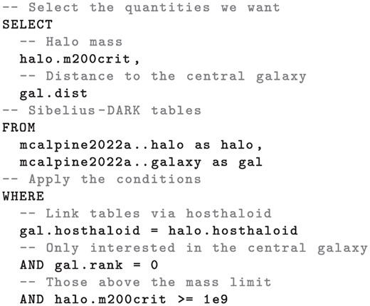
Fig. 9: r-band counts in the North Galactic Cap. This example returns the redshift and apparent r-band magnitude of sibelius-dark galaxies within the North Galactic Cap region of the SDSS survey.

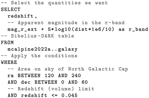
Fig. 16: the Virgo cluster’s member galaxies. This example returns all galaxies with a stellar mass M_* ≥ 10⁸ M_⊙ within 2 Mpc of the sibelius-dark Virgo cluster. This is done in two steps: first, we retrieve the details of the model Virgo cluster knowing the unique galaxyid (listed in Table B2). We then use the retrieved position information to select the galaxies around the model BCG position. This gives us all the information needed to reproduce the left-hand panels of Fig. 16.

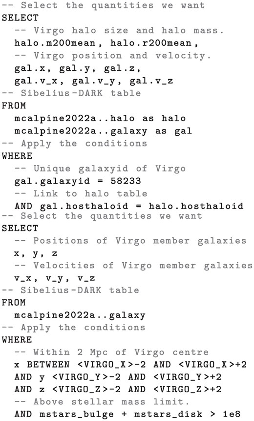
where VIRGO_[X,Y,Z] are the positions of the Virgo cluster found by the first query.

APPENDIX B: CLUSTER AND GALAXY PROPERTIES

Listed in Tables B1 and B2 are the halo and brightest-cluster-galaxy properties for the twelve haloes discussed in Section 3.2. Table B3 shows the properties for the Milky Way and Andromeda analogues discussed in Section 3.4.

Table B1.

The properties of the nine most massive haloes in the sibelius-dark volume, including also the properties of three well known lower mass haloes. Four overdensity masses are listed, along with their enclosed mass radius, where c denotes the critical density and m denotes the mean density. M_rank is the mass ranking of the halo in units of M_200c. The final column shows the observational counterpart cluster for the sibelius-dark halo, identified using Figs 10 and 11. The properties of each haloes most massive subhalo/galaxy (i.e. the BCG) are listed in Table B2.

Object	M200c	M200m	M500c	M500m	r200c	r200m	r500c	r500m	Mrank	Obs. Counterpart
	(1015 M⊙)	(1015 M⊙)	(1015 M⊙)	(1015 M⊙)	(Mpc)	(Mpc)	(Mpc)	(Mpc)		Cat. ID
Perseus	2.72	4.05	1.87	2.97	2.94	4.99	1.91	3.31	1	Abell 426
Hercules-A	1.89	2.93	1.13	2.08	2.60	4.48	1.62	2.94	2	Abell 2199
Hercules-B	1.78	2.46	0.70	2.00	2.56	4.22	1.38	2.91	3	Abell 2151
Norma	1.72	2.19	1.19	1.87	2.53	4.06	1.65	2.84	4	Abell 3627
Coma	1.27	2.04	0.87	1.47	2.28	3.97	1.48	2.62	5	Abell 1656
Leo	1.17	1.42	0.84	1.25	2.22	3.52	1.47	2.48	6	Abell 1367
SD-C7	1.15	1.34	0.88	1.22	2.21	3.45	1.49	2.46	7	–
SD-C8	0.90	1.31	0.61	1.00	2.03	3.43	1.31	2.30	8	–
SD-C9	0.83	1.16	0.53	0.93	1.98	3.29	1.26	2.25	9	Abell 1185
Hydra	0.49	0.73	0.35	0.56	1.66	2.81	1.10	1.90	32	Abell 1060
Centaurus	0.41	0.57	0.30	0.44	1.57	2.59	1.04	1.76	44	Abell 3526
Virgo	0.35	0.48	0.27	0.38	1.49	2.46	1.00	1.67	56	–

Table B2.

The properties of the most massive subhalo/galaxy (i.e. the BCG) hosted by the twelve haloes listed in Table B1. From left to right, the common name for the halo/cluster, the sibelius-dark public data base ID (galaxyid), the subhalo mass (i.e. total bound mass of the subhalo), the distance from the Milky Way, the recession velocity relative to the Milky Way, the galaxy’s right ascension and declination on the sibelius-dark sky, the stellar mass of the galaxy and the central supermassive black hole mass.

Object	galaxyid	Msub	r	vr	RA	DEC	M*	MBH
		(1015 M⊙)	(Mpc)	(km s−1)	(deg)	(deg)	(1011 M⊙)	(109 M⊙)
Perseus	207645	2.81	77.2	5187	44.31	41.87	11.95	34.93
Hercules-A	6720	1.79	141.5	10386	250.11	40.35	10.44	15.19
Hercules-B	2017405	0.66	156.4	11259	241.94	16.99	4.02	4.26
Norma	220176	1.45	73.9	4898	250.91	−59.80	11.81	10.78
Coma	337006	1.22	108.2	7410	196.76	30.13	8.58	5.31
Leo	84853	0.58	100.6	6629	177.23	22.25	7.93	5.83
SD-C7	118936	0.68	180.4	12347	29.53	-0.63	6.28	4.79
SD-C8	8636	0.98	126.5	8690	108.30	-36.79	5.57	11.97
SD-C9	346825	0.63	157.4	10059	167.84	30.27	4.27	6.67
Hydra	37323	0.54	57.5	3516	159.27	−28.50	6.85	6.51
Centaurus	624232	0.45	49.0	3535	197.79	−41.98	4.74	5.38
Virgo	58233	0.35	21.1	1536	196.90	15.96	3.65	3.25

Table B3.

Properties of the two primary Local Group members at z = 0. From left to right, the object name, the sibelius-dark public data base ID (galaxyid), the subhalo mass (i.e. total bound mass of the subhalo), the distance from the Milky Way, the recession and tangential velocity relative to the Milky Way, the galaxy’s right ascension and declination on the Sibelius-DARK sky, the stellar mass of the galaxy, the central supermassive black hole mass and the halo mass. The Milky Way has no reported halo mass (and shares the same hosthaloid in the public data base as the Andromeda galaxy), because the Milky Way and Andromeda are associated with the same Friends-of-Friends group by z = 0 in the simulation, which makes the Milky Way technically a satellite of Andromeda.

Object	galaxyid	Msub	r	vr	vt	RA	DEC	M*	MBH	M200c
		(M⊙)	(Mpc)	(km s−1)	(km s−1)	(deg)	(deg)	(M⊙)	(M⊙)	(M⊙)
Milky Way	17791952	9.42 × 1011	–	–	–	–	–	5.43 × 109	2.62 × 106	–
Andromeda	5098129	1.48 × 1012	0.753	−117	33	25.8	57.5	6.38 × 109	4.40 × 106	1.30 × 1012