BEBOP III. Observations and an independent mass measurement of Kepler-16 (AB) b – the first circumbinary planet detected with radial velocities

ABSTRACT

The radial velocity method is amongst the most robust and most established means of detecting exoplanets. Yet, it has so far failed to detect circumbinary planets despite their relatively high occurrence rates. Here, we report velocimetric measurements of Kepler-16A, obtained with the SOPHIE spectrograph, at the Observatoire de Haute-Provence’s 193cm telescope, collected during the BEBOP survey for circumbinary planets. Our measurements mark the first radial velocity detection of a circumbinary planet, independently determining the mass of Kepler-16 (AB) b to be |$0.313 \pm 0.039\, {\rm M}_{\rm Jup}$|⁠, a value in agreement with eclipse timing variations. Our observations demonstrate the capability to achieve photon-noise precision and accuracy on single-lined binaries, with our final precision reaching |$\rm 1.5~m\, s^{-1}$| on the binary and planetary signals. Our analysis paves the way for more circumbinary planet detections using radial velocities which will increase the relatively small sample of currently known systems to statistically relevant numbers, using a method that also provides weaker detection biases. Our data also contain a long-term radial velocity signal, which we associate with the magnetic cycle of the primary star.

techniques: radial velocities, planets and satellites: detection, planets and satellites: individual: Kepler-16, binaries: eclipsing, binaries: spectroscopic

1 INTRODUCTION

Circumbinary planets are planets that orbit around both stars of a binary star system. Long postulated (Borucki & Summers 1984; Schneider 1994), the first unambiguous discovery of a circumbinary planet came with Kepler-16 (Doyle et al. 2011), detected by identifying three transits within the light curve of an eclipsing binary system monitored by NASA’s Kepler mission (Borucki et al. 2011). Kepler went on to detect another 13 transiting circumbinary planets in 11 systems (Martin 2018; Socia et al. 2020), with another two systems found using TESS (Kostov et al. 2020, 2021). A number of circumbinary planets systems are suspected from eclipse timing variations of binaries on the main sequence (e.g. Borkovits et al. 2016; Getley et al. 2017), and stellar remnants (e.g. Marsh et al. 2013; Han et al. 2017) but most are disputed (e.g. Mustill et al. 2013), and some disproven (e.g. Hardy et al. 2015). Other detections include HD 106906 b, in direct imaging (Bailey et al. 2014) and OGLE-2007-BLG-349L(AB)c with the microlensing method (Bennett et al. 2016).

Despite successes with almost every observational methods, no circumbinary planet signal has been detected using radial velocities yet. In addition, radial velocities have detected many planets with masses compatible with currently known circumbinary planets. This is remarkable since radial velocities are one of the earliest, most established and efficient method of exoplanet detection. The system closest to a circumbinary configuration identified thus far is HD 202206 (Correia et al. 2005; see Section 4).

The radial velocity method has a number of advantages over the transit method. First, it is less restrictive in term of the planet’s orbital inclination thus providing a weaker bias towards short orbital periods. Furthermore, the signal can be obtained at every orbital phase, and the method is more cost-effective and easier to use over a longer term thanks to using ground-based telescopes (Martin et al. 2019). Additionally, radial velocities provide the planet’s mass, its most fundamental parameter. While the transit method can provide a mass when eclipse timing variations are detected, most circumbinary exoplanets unfortunately remain without a robust mass determination with eclipse timing variations mostly providing upper limits (e.g. Orosz et al. 2012; Schwamb et al. 2013; Kostov et al. 2020). Only four of the known circumbinary planets have eclipse-timing mass estimates inconsistent with 0 at >3σ. The present and future TESS and PLATO missions (Rauer et al. 2014; Ricker et al. 2014) are set to identify several more transiting circumbinary planet candidates (e.g. Kostov et al. 2020, 2021). However, these are unlikely to produce many reliable mass measurements, in good part due to rather short observational time-spans compared to Kepler’s.

Overall, radial velocities are essential to create a sample of circumbinary planets that is both greater in number and less biased than the transit sample. This will allow a deeper understanding of circumbinary planets: their occurrence rate (Martin & Triaud 2014), multiplicity (Orosz et al. 2019; Sutherland & Kratter 2019), formation and evolution (e.g. Armstrong et al. 2014; Chachan et al. 2019; Pierens, McNally & Nelson 2020; Penzlin, Kley & Nelson 2021), and dependence on binary properties (Martin, Mazeh & Fabrycky 2015; Muñoz & Lai 2015; Li, Holman & Tao 2016; Martin 2019).

In 2017 we created the BEBOP survey (Binaries Escorted By Orbiting Planets; Martin et al. 2019), as a blind radial velocity survey for circumbinary planets. Prior to this, the most extensive radial velocity effort had been produced by the TATOOINE survey (Konacki et al. 2009), but the survey unfortunately did not yield any discoveries. One issue likely affected the survey, from which BEBOP learnt a great deal: TATOOINE targeted double-lined binaries, which was logical. Double-lined binaries are brighter, both stars can have model independent mass measurements, and one can, in principle, measure the Doppler displacement caused by a planet on each of the two components. However, disentangling both components from their combined spectrum accurately is a complex task, and despite photon noise uncertainties regularly reaching 2 to |$4\, {\rm m\, s}^{-1}$|⁠, the survey returned a scatter of order 15 to |$20 \, {\rm m\, s}^{-1}$| (Konacki et al. 2009, 2010). Indeed, Konacki et al. (2010) recommended single-lined binaries as a solution, but too few were known at the time. Since, radial velocities have been used to constrain the binary parameters, which helps refining the planetary parameters, but not to search for circumbinary planets themselves (e.g. Kostov et al. 2013, 2014).

Thanks to the advent of exoplanet transit experiments, increasing amounts of low-mass single-lined eclipsing binaries are being identified (e.g. Triaud et al. 2013, 2017; von Boetticher et al. 2019; Acton et al. 2020; Lendl et al. 2020; Mireles et al. 2020). The BEBOP survey was constructed solely using sufficiently faint secondaries, to avoid detection with spectrographs such that we could, in principle, reach a radial velocity precision comparable to that around single stars of the same brightness. In principle, this ought to provide an accuracy of order |${1~\rm m\, s}^{-1}$|⁠. Our survey is ongoing, and uses the CORALIE, SOPHIE, HARPS, and ESPRESSO spectrographs. Preliminary results were published in Martin et al. (2019; BEBOP I). In Standing et al. (2021, under review, BEBOP II), we describe our observational protocol, the methods we use to detect planets, as well as how we produce detection limits.

In this paper we detail a complementary project to BEBOP’s blind search. Between 2016 and 2021 we monitored Kepler-16, a relatively bright (Vmag = 12) single-lined eclipsing binary system with a primary mass |$M_{\rm 1} = 0.65~\rm M_\odot$| (a K dwarf), a secondary mass |$M_{\rm 2} = 0.20~\rm M_\odot$| (a mid-M dwarf), and an orbital period |$P_{\rm bin} = 41.1~\rm d$|⁠. The system is |$75~\rm pc$| distant and known to host a circumbinary gas giant planet with a mass |$m_{\rm pl} = 0.33~\rm M_{\rm Jup}$|⁠, and a period |$P_{\rm pl} = 229~\rm d$|⁠. Our observations demonstrate that we can indeed recover the Doppler reflex signature of a circumbinary planet. Our results act to both validate and assist our broader search for new planets. Furthermore, we can derive a ‘traditional’ Doppler mass measurement for the planet, to be compared with that derived from photometric eclipse and transit timings. Finally, our long baseline is sensitive to additional planets, in particular to any that would occupy an orbit misaligned to the transiting inner planets.

2 VELOCIMETRIC OBSERVATIONS ON KEPLER-16

Between 2016-07-08 and 2021-06-23, we collected 143 spectra using the high-resolution high-precision fibre-fed SOPHIE spectrograph, mounted on the 193cm at Observatoire de Haute-Provence, in France (Perruchot et al. 2008). The journal of observations can be found in Table A1. All observations were conducted in HE mode (High Efficiency), where some of the instrumental resolution is sacrificed from 75 000 to 40 000 in favour of a 2.5 times greater throughput. We chose this since whilst Kepler-16 is the brightest circumbinary system, it is relatively faint for SOPHIE, with V ∼ 12.0.

SOPHIE has two fibres: the first stayed on target, while the other was kept on the sky in order to remove any contribution from the Moon-reflected sunlight. Standard calibrations were made at the start of night as well as roughly every 2 h throughout the night to monitor the instrument’s zero-point. In addition, we observed one of three standards (HD 185144, HD 9407, and HD 89269 A) in HE mode nightly, which we used to track and correct for any long-term instrumental drift following procedures established in Santerne et al. (2014) and Courcol et al. (2015).

Our radial velocities were determined by cross-correlating each spectrum with a K5V mask. These methods are described in Baranne et al. (1996), and Courcol et al. (2015), and have been shown to produce precisions and accuracies of a few meters per second (e.g. Bouchy et al. 2013; Hara et al. 2020), well below what we typically obtain on this system. As in Baranne et al. (1996), and Pollacco et al. (2008), we correct our data from lunar contamination by first scaling the calculated CCF (cross-correlation function) on fibre A and B (to account for slightly different efficiencies between the two fibres) before subtracting the two CCFs. This is a particularly important procedure for circumbinary planet searches. Most systems observed with SOPHIE are single stars, and the scheduling software informs the observer whether sunlight reflected on the Moon would create a parasitic cross-correlation signal, with a radial velocity that varies predictably with the lunar phase. In such a situation the observation is postponed. In the case of binary observations, ours, the velocity of the primary star keeps changing by |$\rm km\, s^{-1}$|⁠, meaning we could not practically predict possible lunar contamination at the time of acquisition. We also correct our data from the CTI (charge transfer inefficiency) effect following the procedure described in Santerne et al. (2012).

The cross-correlation software produces two key metrics of the shape of the CCF, its FWHM (full width at half-maximum), and its bisector span (as defined in Queloz et al. 2001). In addition, we measure the |$\rm H\alpha$| stellar activity indicator following Boisse et al. (2009). These are provided in Table A1.

Two measurements are immediately excluded from our analysis. On 2017-09-06 (BJD 2458003.32008) and 2018-10-06 (BJD 2458398.33382), when the fibre was mistakenly placed on to another star. This is obvious from the FWHM we extract from these measurement, and from their radial velocity. They are appropriately flagged in Table A1. In the end, we achieve a mean radial velocity precision of |$\sim 10.6~\rm m\, s^{-1}$| on the remaining 141 measurements.

Radial velocity measurements of the primary have also been obtained with TRES and Keck’s HIRES (Doyle et al. 2011; Winn et al. 2011). These data sets were not used in this analysis for several reasons. First, the TRES data has a mean precision of |$21~ \rm m\, s^{-1}$|⁠, which would be insufficient to detect the planet. Secondly, the HIRES data, despite offering a precision of a few |$\rm m\, s^{-1}$|⁠, was only taken on a single night and is contaminated by the Rossiter–McLaughlin signal of the eclipse. Finally, by solely using our own SOPHIE data we may produce a near independent detection. In a similar spirit, we do not use any of Kepler’s or TESS’s photometric data to conduct our search and parameter estimation.

Finally, Bender et al. (2012) collected near-infrared spectra to reveal the secondary’s spectral lines (i.e. observing Kepler-16 as a double-lined spectroscopic binary). Similarly, we do not use these measurements in our analysis, although we do use their estimate for the primary mass.

3 MODELLING OF THE RADIAL VELOCITIES

In order to ascertain our capacity to detect circumbinary planets using radial velocities, as an independent method, we decided to use two different algorithms with different methods for measuring a detection probability. Before describing this, we will detail our procedure to remove outliers. As a reminder, we only use SOPHIE data (see above), where Kepler-16 appears as a single-lined binary and we only observe the displacement of the primary star around the system’s barycentre.

3.1 Outlier removal

We searched our 141 data for measurements¹ coinciding with a primary eclipse, and likely affected by the Rossiter–McLaughlin effect (McLaughlin 1924; Rossiter 1924; Winn et al. 2011; Triaud 2018). Fortunately no measurements needed to be excluded for this reason.

We also realized that a number of measurements were likely taken under adverse conditions. This is apparent from an unusually low signal-to-noise ratio, but also from large values of the bisector span. Typically used as a stellar activity, or a blend indicator (Queloz et al. 2001; Santos et al. 2002), the span of the bisector slope (bisector span, or bis span) effectively informs us that the line shape varied and therefore that the mean of the cross-correlation function is likely affected. We took the mean of the bisector span measurement and removed all measurements in excess of 3σ away from the mean. Five measurements are excluded this way, all with a bisector span |$\gtrsim \pm 100~\rm m\, s^{-1}$|⁠. Excluded measurements are reported in the journal of observations in Table A1 with a flag.

For visual convenience we also exclude one measurement taken on 2018-06-02 (BJD 2458271.53928) on account of its very low signal to noise and correspondingly large uncertainty, seven times greater than the semi-amplitude of Kepler-16 b. Again, this is reported in Table A1 with a flag.

Finally, we remove a measurement obtained on 2017-10-30 (BJD 2458057.38946). This measurement is ∼6σ away from the best-fitting model. It is totally unclear why this is the case since its FWHM, bisector span, and |$\rm H\alpha$|⁠, all appear compatible with other measurements.

After removing these seven outliers, our analysis is performed on the remaining 134 SOPHIE measurements. The exoplanet detection described just below is done twice, without, and with the seven outlying measurements. Their exclusion did not affect our conclusion but refined our parameters. We also reproduced the following fitting procedures by including the previously existing TRES and HIRES data with no discernible differences.

3.2 Analysis using the genetic algorithm Yorbit

Yorbit is a radial velocity fitting tool used for exoplanet detection, described in Ségransan et al. (2011). It assumes Keplerian orbits (see Section 3.5). Yorbit first performs a Lomb–Scargle periodogram of the observations, which is then used to initiate a genetic algorithm that iterates over the orbital period P, the eccentricity e, the argument of periastron ω, the semi-amplitude K, a reference time T₀, and one systemic velocity per data set γ (for conventions, see Hilditch 2001). Once the algorithm has converged on a best solution, the final parameters are estimated by using a least-square fit. The tool has been routinely used to identify small planetary companions successfully (e.g. Mayor et al. 2011; Bonfils et al. 2013), and represents a more traditional, and possibly a more recognized way of identifying a new planetary system than the nested sampler we use subsequently (see Section 3.3). However, Yorbit cannot do a Bayesian model comparison. Instead it computes a false alarm probability (FAP) by performing a bootstrap on the data thousands of times and computing for each iteration a Lomb–Scargle periodogram.

In a first instance, just one Keplerian is adjusted to the SOPHIE data, with Yorbit automatically finding the most prominent signal, that of the secondary star. Following this step, we remove the secondary’s signal and search the resulting residuals with a periodogram. This periodogram shows excess power around 230 d with a |$\rm FAP~\sim 0.1{{\ \rm per\ cent}}$| as well as excess power for a signal longer than the range of dates we observed for, which we later associate to a magnetic cycle. To isolate the signal of Kepler-16 b, we fit the secondary’s Keplerian to the data, alongside a polynomial function, which is used to detrend that longer signal. Once Yorbit has converged, we search the residuals again with a periodogram, which provides a |$\rm FAP~\ll 0.01{{\ \rm per\ cent}}$| (Fig. 1), clearly detecting Kepler-16 b as an additional periodic sinusoidal signal. The FAP obtained with a cubic detrending function is one order of magnitude better than that obtained with a quadratic function, so we chose the former as our baseline detrending.

Figure 1.

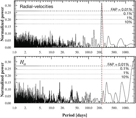
Lomb–Scargle periodogram of Kepler-16’s radial velocities (top) and |$\rm H\alpha$| (bottom). The radial velocities are shown after removing the binary motion, and a cubic function. The four lines are, from bottom to top, the |$10{{\ \rm per\ cent}}$|⁠, |$1{{\ \rm per\ cent}}$|⁠, |$0.1{{\ \rm per\ cent}}$|⁠, and |$0.01{{\ \rm per\ cent}}$| FAP. There is a highly significant peak around 230 d (vertical red dotted line) that is present in the radial velocities but not in |$\rm H\alpha$|⁠. The |$\rm H\alpha$| measurements contain significant periodogram power at |$\gtrsim 2000~\rm d$|⁠, indicating a long-term trend in the chromospheric emission from the primary star.

To obtain results on the system’s parameters, we perform a final fit to the data assuming two Keplerians and a cubic detrending function. Results of that fit are found in Table 1. The orbital parameters of the planet are compatible with those produced in Doyle et al. (2011; see Table 1 and Section 3.5 for a discussion). Our final fit produces a reduced |$\chi ^2_\nu = 1.17\pm 0.14$|⁠, implying no additional complexity is needed to explain the data, and supporting our choice for a circular planetary orbit.² In addition, this shows that we can achieve photon-noise precision on single-lined binary to detect circumbinary planets. The model fit to the data is depicted in Fig. 2.

Figure 2.

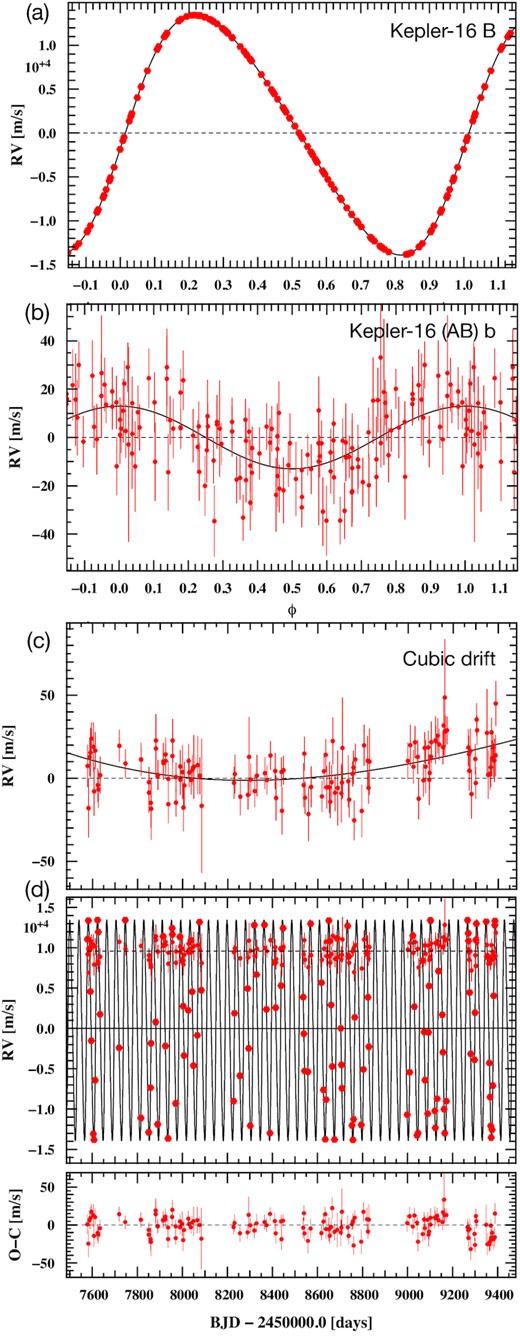
Best-fitting adjustment to the SOPHIE radial velocity data. a: Doppler reflex motion caused by the secondary star. b: Doppler reflex motion caused by the circumbinary planet. c: Cubic drift associated with a magnetic cycle. d: Radial velocities as a function of time with a binary+planet+cubic function model. Residuals are displayed below.

Table 1.

Results of our analysis of the SOPHIE radial velocities only, after removing outliers, that show the fit’s Jacobi parameters and their derived physical parameters. They are compared to previous results with 1σ uncertainties provided in the form of the last two significant digits, within brackets. Dates are given in BJD – 2450000. We adopt the Kima column as our results.

Parameters & units		Yorbit	Kima	Doyle+ (2011)
Binary parameters
Pbin	day	41.077779(54)	41.077772(51)	41.079220(78)
|$T_{0, \rm bin}$|	BJD	8558.9640(44)	7573.0984(47)	–
|$K_{1, \rm bin}$|	|$\rm m\, s^{-1}$|	13 678.2(1.5)	13 678.7(1.5)	–
ebin	–	0.15989(11)	0.15994(10)	0.15944(62)
ωbin	deg	263.661(40)	263.672(40)	263.464(27)
Planet parameters
Ppl	day	228.3(1.8)	226.0(1.7)	228.776(37)
|$T_{0, \rm pl}$|	BJD	8532.5(4.4)	7535(92)	–
|$K_{1, \rm pl}$|	|$\rm m\, s^{-1}$|	12.8(1.5)	11.8(1.5)	–
epl	–	0 (fixed)	<0.21	0.0069(15)
ωpl	deg	–	231(65)	|$318^{(+10)}_{(-22)}$|
System parameters
γ	|$\rm km\, s^{-1}$|	−33.8137(69)	−33.8065(45)	−32.769(35)
σjitter	|$\rm m\, s^{-1}$|	–	0.070 |$^{+1.104}_{-0.067}$|	–
Derived parameters
M1	|$\rm M_\odot$|	0.654(17)*	0.654(17)*	0.6897(35)
M2	|$\rm M_\odot$|	0.1963(31)	0.1964(31)	0.20255(66)
mpl	|$\rm M_{Jup}$|	0.345(41)	0.313(39)	0.333(16)
abin	|$\rm AU$|	0.2207(18)	0.2207(17)	0.22431(35)
apl	|$\rm AU$|	0.6925(67)	0.6880(58)	0.7048(11)

Note. *adopted from Bender et al. (2012)

Including seven outliers described in Section 3.1, neither the FAP nor the reduced |$\chi ^2_\nu$| are significantly affected.

3.3 Analysis using the diffusive nested sampler Kima

Kima is a tool developed by Faria et al. (2018), which fits a sum of Keplerian curves to radial velocity data. It samples from the posterior distribution of Keplerian model parameters using a diffusive nested sampling algorithm by Brewer & Foreman-Mackey (2016). Diffusive nested sampling allows the sampling of multimodal distributions, such as those typically found in exoplanetary science and radial velocity data (Brewer & Donovan 2015), evenly and efficiently.

Kima can treat the number of planetary signals (N_p) present in an RV data set as a free parameter in its fit. Since the tool also calculates the fully marginalized likelihood (evidence), it allows for Bayesian model comparison (Trotta 2008) between models with varying N_p. A measure of preference of one Bayesian model over another can be ascertained by computing the ‘Bayes Factor’ (Kass & Raftery 1995) between the two. The Bayes factor is a ratio of probabilities between the two competing models. Once a value for the Bayes factor has been calculated, we can compare it to the so-called ‘Jeffreys’ scale’ (see Trotta 2008 for more details) to rate the strength of evidence of one model over another.

A more extensive description of our use of Kima in the context of the BEBOP survey can be found in Standing et al. (2021). For the analysis of the Kepler-16 system, prior distributions were chosen similarly to those used in Faria et al. (2020) with the following notable adaptions. We treat the secondary star as a known object with tight uniform priors on its orbital parameters. A log-uniform distribution was used to describe the periods of any additional signals, from 4 × P_bin to 1 × 10⁴ d. This inner limit on period is set by the instability limit found in binary star systems (Holman & Wiegert 1999). More details, particularly on the priors we use, can be found in Standing et al. (2021). Just like for the previous analysis using Yorbit, Kima is only deployed on SOPHIE data, and excluding outliers described in Section 3.1.

Our Kima analysis of the Kepler-16 data yields a Bayes Factor |$\rm BF \gt 10000$| in favour of a three Keplerian model (secondary star, planet, and cubic drift). Our posterior shows overdensities at orbital periods of ≈230 and ≈2000 d, corresponding to the signal of Kepler-16 b and the cubic drift seen in Yorbit. We then apply the clustering algorithm hdbscan (McInnes, Healy & Astels 2017) to isolate and extract the resulting planetary orbital parameters, which can be found in Table 1.

3.4 Note on converting fitted parameters to physical values

To convert our semi-amplitudes into masses for M₂ and m_pl, for the secondary star and planet masses (respectively), we adopt a primary star mass (M₁) from Bender et al. (2012). Software written for exoplanetary usage usually assumes that m_pl ≪ M_⋆ (including Yorbit and Kima); however, this assumption is no longer valid when comparing M₂ to M₁, and a circumbinary planet to both.

First, we find M₂ iteratively using the mass function, following the procedure described in Triaud et al. (2013). Then, we estimate m_pl from |$K_{1,\rm pl}$| by using the combined mass M₁ + M₂. This is because whilst we are only measuring the radial velocity signature of the primary star, the gravitational force of the planet acts on the barycentre of the binary. Had we not done this extra conversion step, we would find significant differences, with erroneous |$M_2 = 0.165~\rm M_\odot$| and |$m_{\rm pl} = 0.29~\rm M_{Jup}$| for the Yorbit results.

Differences between our derived parameters (bottom part of Table 1) and those from Doyle et al. (2011) are mainly explained by our adoption of the more accurate M₁ mass from Bender et al. (2012) rather than using the value from Doyle et al. (2011).

3.5 Note on circumbinary planets’ orbital elements

The main differences between our fitted parameters and those from Doyle et al. (2011) are caused by our parameters being akin to mean parameters (e.g. the mean orbital period), whereas Doyle et al. (2011) provide osculating parameters, which are the parameters the system had at one particular date, and which constantly evolve following three-body dynamics (Mardling 2013). Also, the planetary signal is significantly more obvious in the Kepler transiting data than in our radial velocities. Each measurement within a planetary transit over the primary star produces an |$\rm SNR = 243$| (⁠|$\rm SNR=14$| when over the secondary). This is why Kepler can derive osculating elements, by solving Newton’s equations of motion: the planetary motion is resolved orbit after orbit (transit after transit). Comparatively, our radial velocity observations have required multiple orbits of the planet to build up a significant detection. We can therefore only measure a mean period, and are justified in using software which can only adjust non-interacting Keplerian functions.

For example, Doyle et al. (2011) provide a highly precise value of P_pl = 228.776 ± 0.037 d, yet this osculating period will vary by approximately ±5 d over a time-scale of just years. Our measured period of P_pl = 226.0 ± 1.7 d has a much higher error with this uncertainty being a combination of our radial velocities being less constraining on the period, and our assumption of a static orbit. The value we obtain with Kima is 1.6σ compatible with the value found by Doyle et al. (2011).

With respect to the planet mass, we can derive a value with similar precision to that of Doyle et al. (2011) because whilst the transit signature of the planet is much stronger than its radial velocity signature, the transit signature itself carries very little information about the planet’s mass. The photodynamical mass derived in Doyle et al. (2011) is dictated by the eclipse timing variations, which have an amplitude of a couple of minutes and have a precision on the order of tens of seconds, producing an SNR close to our radial velocities.

Finally, to validate our assumption that we cannot measure osculating elements with our current data, we used tools described in Correia et al. (2005, 2010) to perform an N-body fit to the radial velocities. This fit finds no improvements in χ² indicating that Newtonian effects indeed remain below the detectable threshold.

3.6 A magnetic cycle, and constraints on additional planets

To assess the presence of an external companion causing the additional polynomial signal we notice in our data, we force a two-Keplerian model to fit the data (a circular orbit for the planet and a free-eccentricity orbit for the binary) and analyse the residuals. We find a signal reaching a |$\rm FAP~\lt 0.01{{\ \rm per\ cent}}$| at orbital periods exceeding the time-span of our data (⁠|$\gtrsim 2,000 \rm ~d$|⁠). Long-term drifts can sometimes be caused by magnetic cycles since stellar spots and faculae tend to suppress convective blue-shift, producing a net change in the apparent velocity of a star (Dravins 1985; Meunier, Desort & Lagrange 2010; Dumusque et al. 2011). We perform a Lomb–Scargle periodogram on the |$\rm H\alpha$| activity indicator we extracted from the SOPHIE spectra, and find a |$\rm FAP\lt 0.01{{\ \rm per\ cent}}$|⁠. We therefore interpret this long-term radial velocity drift as a magnetic cycle, with a time-scale longer than the time-span of our observations.

The validity of this interpretation can be tested since duration of stellar magnetic cycles scales with stellar rotation periods (for single star; Suárez Mascareño, Rebolo & González Hernández 2016). We measure the primary star’s rotation from the vsin i₁ obtained during the Rossiter–McLaughlin effect by Winn et al. (2011) to the primary’s stellar radius obtained by Bender et al. (2012) and obtain a primary rotation |$P_{\rm rot,1} = 35.68\pm 1.04~\rm d$|⁠. Following the relation of Suárez Mascareño et al. (2016), with the observed stellar rotation we ought to expect a magnetic cycle on a time-scale of 1900 to 2400 d, which is entirely compatible with the |$\rm H\alpha$| signal and the long-term radial velocity drift.

We now use Kima as done in Standing et al. (2021) to compute a detection limit on the presence of additional but undetected planetary companions. We first remove the highest likelihood model with two Keplerians (the planet and the long-term drift) from the data, then force N_p = 1 to obtain a map of all remaining signals that are compatible with the data, but remain formally undetected (the binary is also adjusted at each step). This map is shown as a grey-scale density on Fig. 3. The |$99{{\ \rm per\ cent}}$| contour informs us that we are sensitive to companions below the mass of Kepler-16 b up to orbital periods of ∼3000 d. This complements Martin & Fabrycky (2021)’s work who placed detection limits down to Earth-radius planets but only out to periods of 500 d, re-analysing the Kepler photometry.

Figure 3.

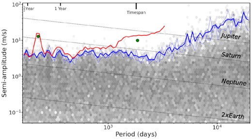
Detection sensitivity to additional planets plotted as semi-amplitude |$K_{1,\rm pl}$| as a function of P_pl. The hexagonal bins depict the density of posterior samples obtained from three separate Kima runs applied on the Kepler-16 radial velocity data after removing two Keplerian signals shown with green dots. The faded blue lines show detection limits calculated for each of the three runs on the system. The solid blue line shows the detection limit calculated from all posterior samples combined. The solid red line is the outline of the posterior that led to the detection of Kepler-16 b and of a long-term trend associated with a magnetic cycle. The green dots represent the two signals removed from the data to compute the blue detection limit.

Overall, a picture is emerging of Kepler-16 b as a lonely planet, which has implications for the formation and migration of multiplanet systems in the presence of a potentially destabilising binary (e.g. Sutherland & Kratter 2019).

4 DISCUSSION

Our data clearly shows an independent detection of the circumbinary planet Kepler-16 b, the first time a circumbinary planet is detected using radial velocities, and the first time a circumbinary planet is detected using ground-based telescopes as well. We re-iterate that our model fits are solely made using radial velocities and completely ignore any Kepler or other photometric data, to emulate BEBOP’s blind search. Importantly, our results show we can achieve a precision close to |$\rm 1~m\, s^{-1}$| on a planetary signal, with the 1σ uncertainties on the semi-amplitudes being only just |$\rm 1.5~m\, s^{-1}$|⁠. This is compatible with the semi-amplitudes of super-Earths and sub-Neptunes (e.g. Mayor et al. 2011). The closest previous detection to a circumbinary planet made from the ground was produced by Correia et al. (2005) on HD 202206, a system comprised of a Sun-like star with an inner companion with mass |$m_b\sin i_b = \rm 17.4~M_{Jup}$| and orbital period |$P_b = 256~\rm d$|⁠, and an outer companion with mass |$m_c\sin i_c = \rm 2.44~M_{Jup}$| and orbital period |$P_c = 1383~\rm d$|⁠. Benedict & Harrison (2017) claim an astrometric detection of the system that implies a nearly face-on system, with |$m_b = 0.89~\rm M_\odot$| and |$m_c = 18~\rm M_{Jup}$|⁠, suggesting a circumbinary brown dwarf. However, a dynamical analysis produced by Couetdic et al. (2010) imply such a configuration is unstable and therefore unlikely, favouring instead a more edge-on system.

We first detect Kepler-16 b by using a classical approach to planet detection, via periodograms and FAP, but also perform a second analysis using the diffusive nested sampler Kima, which allows to perform model comparison and model selection in a fully Bayesian framework. Kima will be the method of choice for the remainder of the BEBOP survey Standing et al. (2021). The parameters for the planetary companion are broadly compatible with those measured at the time of detection by Doyle et al. (2011), and which have not been revised since. With our current precision it is not possible to determine the eccentricity of the orbit, but we can place an upper limit on it.

Finally, we discuss the detectability of circumbinary systems. We only take the 20 first measurements we collected and run Kima measuring the Bayes Factor to assess the detectability of Kepler-16 b, where individual uncertainties are similar to the semi-amplitude of the signal, |$K_{1,\rm pl}$|⁠. We repeat the procedure, measuring BF for each increase of five measurements until we reach a sub-sample containing the 50 first radial velocity measurements (they roughly cover four orbital periods of the planet). We reach a BF >150 (the formal threshold for detection) with the first 40 measurements. We repeat this procedure but instead randomly select 50 measurements within the first 3 yr of data. We run Kima and measure the Bayes Factor for the first 20 epochs of this sequence of 50 random epochs. We then increase from 20 to 25 until reaching 50. We find that the BF =150 threshold is also passed at 40 measurements. We plot our results in Fig. 4. The results between both series of tests are broadly consistent, except when we only use 25 measurements, with the Bayes Factor growing log-linearly with increasing number of measurements. Thanks to these tests we conclude that just 40 to 45 measurements would have been to formally detect Kepler-16 b with radial velocities.

Figure 4.

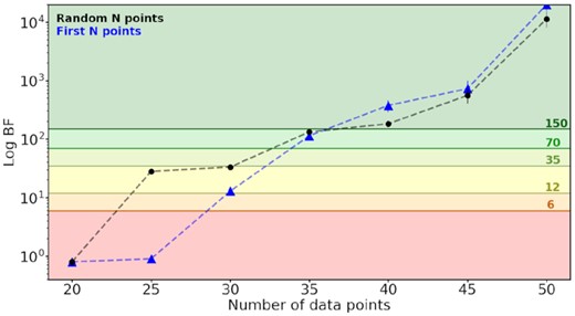
Bayes factors obtained for subsets of data with increasing size. The blue line and triangles indicate the Bayes factors obtained by running Kima on the first N data points obtained on Kepler-16. The black line and dots show the same but for randomly sampled N data points within the first 3 yr of data. Coloured regions represent various thresholds corresponding to improvements in evidence in favour of the more complex binary + planet model as per the Jeffreys’ scale detailed in Standing et al. (2021).

SUPPORTING INFORMATION

Please note: Oxford University Press is not responsible for the content or functionality of any supporting materials supplied by the authors. Any queries (other than missing material) should be directed to the corresponding author for the article.

ACKNOWLEDGEMENTS

First, we would like to thank the staff, in particular the night assistants, at the Observatoire de Haute-Provence for their dedication and hard work, particularly during the COVID pandemic. Secondly, we wish to thank our reviewer, David Armstrong, for reading and commenting our paper. The data were obtained first as part of a DDT graciously awarded by the OHP director (Prog.ID 16.DISC.TRIA), and then by a series of allocations through the French PNP (Prog. IDs 16B.PNP.HEB2, 17A.PNP.SANT, 17B.PNP.SAN2, 18A.PNP.SANT, 18B.PNP.SAN1, 19A.PNP.SANT). The French group acknowledges financial support from the French Programme National de Planétologie (PNP, INSU). This research received funding from the European Research Council (ERC) under the European Union’s Horizon 2020 research and innovation programme (grant agreement no. 803193/BEBOP) and from the Leverhulme Trust (research project grant no. RPG-2018-418). EW acknowledges support from the ERC Consolidator Grant funding scheme (grant agreement no. 772293/ASTROCHRONOMETRY). Support for this work was provided by NASA through the NASA Hubble Fellowship grant number HF2-51464 awarded by the Space Telescope Science Institute, which is operated by the Association of Universities for Research in Astronomy, Inc., for NASA, under contract NAS5-26555. PC thanks the LSSTC Data Science Fellowship Program, which is funded by LSSTC, NSF Cybertraining Grant #1829740, the Brinson Foundation, and the Moore Foundation; her participation in the program has benefited this work. SH acknowledges CNES funding through the grant 837319. ACC acknowledges support from the Science and Technology Facilities Council (STFC) consolidated grant number ST/R000824/1. ACMC acknowledges support by CFisUC projects (UIDB/04564/2020 and UIDP/04564/2020), GRAVITY (PTDC/FIS-AST/7002/2020), ENGAGE SKA (POCI-01-0145-FEDER-022217), and PHOBOS (POCI-01-0145-FEDER-029932), funded by COMPETE 2020 and FCT, Portugal.

The radial velocity data are included in the appendix of this paper. The reduced spectra are available at the SOPHIE archive: http://atlas.obs-hp.fr/sophie/. Data obtained under Prog.IDs 16.DISC.TRIA, 16B.PNP.HEB2, 17A.PNP.SANT, 17B.PNP.SAN2, 18A.PNP.SANT, 18B.PNP.SAN1, and 19A.PNP.SANT.

Footnotes

1

The first series of 14 measurements were obtained from a catalogue containing erroneous proper motions and epochs, which in turn created a |$1.5~\rm km\, s^{-1}$| effect in the radial velocity as the Earth’s motion was overcompensated. This can be corrected easily, but the error remains within the archival data.

2

Making a fit with a quadratic function we obtain |$\chi ^2_\nu = 1.47\pm 0.15$|⁠, for one fewer parameter, justifying our choice for the cubic drift.

APPENDIX A: JOURNAL OF OBSERVATIONS

Table A1.

Journal of observations containing our SOPHIE data. Flags indicate whether the measurement are excluded from our fiducial analysis with the following reason: W, wrong star; B, bisector outlier; U, high uncertainty; O, other. Dates are given in BJD – 2400000. V_rad are the measured radial velocities with their uncertainties |$\sigma _{V_{\rm rad}}$|⁠. FWHM is the Full With at Half Maximum of the Gaussian fitted to the cross correlation function, and contrast is its amplitude. Bis. span is the span of the bisector slope. Uncertainties on FWHM and bis. span are |$2\times \sigma _{V_{\rm rad}}$|⁠. H_α is the equivalent width of H_α, and its uncertainty |$\sigma _{H_\alpha }$|⁠.

flag	BJD-2400000	Vrad	|$\sigma _{V_{\rm rad}}$|	FWHM	contrast	bis. span	Hα	|$\sigma _{H_\alpha }$|
	[days]	[|$\rm km\, s^{-1}$|]	[|$\rm km\, s^{-1}$|]	[|$\rm km\, s^{-1}$|]		[|$\rm km\, s^{-1}$|]
	57578.42404	−22.7567	0.0126	10.4138	22.7274	−0.0233	0.2119	0.0022
B	57581.57256	−20.3465	0.0444	10.4924	13.0881	−0.1227	0.2184	0.0055
	57582.52743	−20.4322	0.0176	10.3201	27.2220	−0.0199	0.2046	0.0036
	57587.43166	−23.9495	0.0113	10.2935	25.8863	0.0192	0.2031	0.0021
	57591.44122	−29.2376	0.0146	10.2883	26.1452	0.0538	0.2117	0.0029
	57595.47979	−35.3428	0.0096	10.3340	29.0424	0.0125	0.2039	0.0020
	57604.43905	−46.8841	0.0145	10.4605	25.3376	−0.0054	0.2147	0.0028
	57607.38886	−47.6294	0.0145	10.4123	28.2874	0.0037	0.2135	0.0030
	57612.47728	−40.2406	0.0110	10.3402	28.9602	0.0079	0.2116	0.0023
	57623.37736	−20.3825	0.0100	10.2928	29.0664	−0.0093	0.2032	0.0020
	57626.38491	−21.8607	0.0110	10.3395	28.9280	0.0329	0.2063	0.0022
	57634.40704	−32.0631	0.0109	10.3925	28.9876	−0.067	0.2092	0.0023
	57719.26505	−36.2183	0.0095	10.3290	28.9030	0.0201	0.1966	0.0018
	57746.26923	−20.3795	0.0084	10.3404	29.0733	−0.0067	0.2122	0.0016
	57815.65363	−44.9376	0.0098	10.3132	27.1330	−0.0004	0.2095	0.0018
	57815.67731	−44.8993	0.0083	10.3249	29.1040	0.0086	0.2080	0.0016
	57850.59947	−46.6829	0.0091	10.3250	27.0881	0.0033	0.2069	0.0017
	57850.62308	−46.7070	0.0119	10.2789	28.0442	−0.0021	0.2067	0.0022
	57858.58652	−41.1658	0.0146	10.2378	23.9695	−0.0255	0.1882	0.0025
	57860.61247	−35.6563	0.0186	10.2443	23.5034	0.0100	0.1941	0.0032
	57881.49587	−33.0003	0.0175	10.2694	22.2896	−0.0211	0.2216	0.0030
	57881.51944	−33.0316	0.0158	10.2409	25.8066	0.0089	0.2109	0.0029
	57890.53416	−45.6792	0.0089	10.2779	27.3843	0.0160	0.1951	0.0016
	57890.57816	−45.7231	0.0081	10.2384	27.7725	−0.0009	0.1910	0.0015
	57914.55102	−22.4041	0.0110	10.2004	25.3872	−0.0078	0.2151	0.0020
	57914.57472	−22.4272	0.0084	10.2139	27.9878	0.0084	0.2134	0.0016
	57924.49590	−35.9753	0.0099	10.2853	27.2617	0.0267	0.1996	0.0018
	57924.52118	−36.0181	0.0103	10.2534	28.8795	0.0171	0.2012	0.0020
	57936.48767	−47.4623	0.0106	10.2734	26.9318	0.0141	0.1932	0.0020
	57936.51133	−47.4660	0.0113	10.3536	28.5829	−0.0057	0.1917	0.0021
	57954.37721	−21.3857	0.0134	10.2930	25.3470	0.0145	0.2031	0.0024
	57955.36873	−22.1650	0.0129	10.2899	25.3384	−0.0119	0.2043	0.0022
	57970.44413	−43.0893	0.0085	10.2438	28.2732	0.0268	0.1914	0.0016
	57970.46806	−43.1358	0.0082	10.2520	28.9462	0.0077	0.1877	0.0015
	57989.42736	−22.4627	0.0097	10.2269	27.1918	0.0127	0.1965	0.0017
	57989.45189	−22.4383	0.0091	10.2555	29.0876	−0.0119	0.1930	0.0017
	57999.37737	−25.3762	0.0160	10.2317	23.9715	−0.0013	0.1971	0.0027
W	58003.32008	−3.1611	0.0199	7.5424	24.2589	0.0161	0.2016	0.0045
	58003.42095	−31.0632	0.0141	10.1974	23.2722	−0.0428	0.1954	0.0023
	58007.42352	−37.1754	0.0142	10.3020	28.2437	0.0059	0.1924	0.0027
	58026.32236	−31.5767	0.0100	10.2828	26.6464	0.0082	0.2004	0.0018
	58029.34747	−24.2823	0.0086	10.2444	31.1481	−0.0078	0.1962	0.0018
B	58034.33565	−20.4064	0.0114	10.2145	31.4902	−0.0954	0.1925	0.0024
	58038.28757	−22.8921	0.0085	10.2171	29.0859	−0.0010	0.1947	0.0016
	58043.30107	−29.2555	0.0088	10.1869	27.6237	0.0084	0.1888	0.0016
	58049.33656	−38.4188	0.0190	10.3105	23.6222	−0.0004	0.2151	0.0033
O	58057.38946	−47.4170	0.0127	10.3516	27.6078	0.0028	0.1924	0.0022
	58066.32858	−34.6758	0.0173	10.2573	23.9592	0.0012	0.2000	0.0029
	58076.24290	−20.6229	0.0109	10.2381	26.3816	0.0227	0.1993	0.0020
	58084.24172	−29.0736	0.0402	10.3369	17.3316	0.0183	0.2143	0.0061
	58227.56803	−42.8215	0.0095	10.3294	29.2382	0.0159	0.1975	0.0018
	58231.59284	−31.9304	0.0115	10.3272	28.2728	−0.0126	0.1911	0.0022
	58255.55341	−39.6783	0.0111	10.2862	26.8276	−0.0023	0.1972	0.0020
U	58271.53928	−35.2297	0.0775	10.4414	14.1731	0.0514	0.2170	0.0113
	58289.48662	−28.8597	0.0086	10.2324	27.6608	0.0124	0.1940	0.0016
	58294.41403	−36.2932	0.0238	10.1405	19.6541	−0.0463	0.1980	0.0038
	58301.52589	−45.8824	0.0094	10.2594	27.0071	−0.0092	0.1856	0.0017
	58319.49236	−21.0086	0.0095	10.232	27.3731	−0.0159	0.1864	0.0017
	58329.35035	−27.1417	0.0123	10.1726	26.8217	0.0135	0.1895	0.0024
	58364.49871	−20.9710	0.0095	10.2804	29.4757	0.0077	0.1917	0.0018
	58373.38714	−31.4460	0.0085	10.2349	28.9319	−0.0064	0.1959	0.0017
	58389.28389	−46.7948	0.0085	10.2759	28.4801	−0.0032	0.1936	0.0017
W	58398.33382	2.0217	0.0162	7.6074	33.8799	−0.0066	9999.99	9999.99
	58410.34703	−25.6250	0.0107	10.2377	30.7540	0.0084	0.1970	0.0023
	58414.31942	−31.2461	0.0135	10.2164	26.4540	−0.0110	0.2059	0.0026
	58438.23468	−28.5063	0.0086	10.2149	28.7501	−0.0001	0.2048	0.0017
	58440.32791	−23.9560	0.0141	10.4258	30.7245	0.0284	0.2063	0.0030
	58447.28753	−21.3746	0.0085	10.2282	30.6147	−0.0060	0.1972	0.0018
	58536.69186	−29.9300	0.0131	10.2127	26.6076	−0.0381	0.1960	0.0026
	58539.69622	−34.4673	0.0101	10.3190	28.0285	−0.0214	0.1959	0.002
	58542.70128	−39.0813	0.0096	10.2536	28.4771	−0.0302	0.2042	0.0019
	58557.68116	−39.1923	0.0161	10.2757	27.2871	0.0405	0.2019	0.0033
	58569.61968	−20.8305	0.0122	10.2296	27.7821	−0.0081	0.2002	0.0024
	58617.59111	−28.1421	0.0091	10.2460	28.7484	−0.0038	0.2015	0.0018
	58626.46789	−41.4286	0.0107	10.2794	25.8409	0.0075	0.2010	0.0020
	58634.53897	−47.5651	0.0093	10.2481	26.5013	−0.0039	0.2018	0.0018
	58638.43325	−42.6407	0.0126	10.2794	28.4741	−0.0223	0.2039	0.0026
	58650.53936	−20.4374	0.0152	10.1724	26.3894	0.0132	0.2030	0.0031
	58654.49571	−22.9659	0.0097	10.2282	28.3680	−0.0006	0.1971	0.0019
	58660.56745	−30.9076	0.0102	10.2163	28.9174	−0.0113	0.1984	0.0022
	58665.57318	−38.5290	0.0140	10.2965	27.5442	0.0455	0.1981	0.0028
	58675.57952	−47.5981	0.0109	10.3365	27.6547	0.0017	0.1965	0.0022
	58687.61864	−22.6485	0.0225	10.3376	23.7336	0.0388	0.2054	0.0043
	58703.54677	−33.7950	0.0175	10.3134	26.0287	0.0192	0.2010	0.0036
	58706.50803	−38.3266	0.0100	10.2295	28.0761	−0.0120	0.1982	0.0020
	58708.50232	−41.2314	0.0301	10.2930	16.0707	−0.0426	0.1994	0.0047
B	58732.43751	−20.3947	0.0302	10.2203	25.1441	−0.1346	0.2322	0.0062
	58734.44238	−21.1078	0.0155	10.2528	27.1499	−0.0207	0.2124	0.0031
	58738.38163	−24.8845	0.0105	10.1784	27.7775	−0.0244	0.2003	0.0021
	58753.33846	−45.8380	0.0075	10.2737	28.6564	−0.0095	0.202	0.0016
	58757.43639	−47.6475	0.0099	10.3475	28.4233	0.0141	0.2001	0.0020
	58760.37181	−45.0829	0.0118	10.2839	28.1836	0.0119	0.1973	0.0024
	58765.41646	−32.4426	0.0094	10.2947	28.2387	0.0005	0.2029	0.0019
	58794.31837	−45.7701	0.0157	10.3120	26.8288	−0.0071	0.2012	0.0031
	58804.24157	−38.9032	0.0122	10.3048	27.9886	0.0424	0.2025	0.0024
	58820.22529	−24.4962	0.0149	10.3393	26.6102	−0.0071	0.2153	0.0030
	58824.24004	−29.9520	0.0094	10.2552	28.2000	0.0245	0.2090	0.0019
	58828.27635	−36.0832	0.0198	10.4292	23.1762	−0.0434	0.2019	0.0034
B	58919.69124	−47.3685	0.0208	10.3504	24.6286	−0.1229	0.2077	0.0041
	58998.56140	−44.5035	0.0109	10.3115	28.8681	0.0086	0.1939	0.0022
	59009.49993	−39.2485	0.0122	10.2756	27.7224	−0.0107	0.2039	0.0025
	59023.55894	−22.3117	0.0099	10.2759	28.5419	−0.0080	0.1996	0.0019
	59030.43413	−31.1164	0.0095	10.2358	28.4005	0.0120	0.1979	0.0019
	59042.42642	−47.0737	0.0101	10.2934	28.2747	0.0043	0.2012	0.0020
	59046.54366	−46.7980	0.0123	10.2777	28.0726	−0.0441	0.1967	0.0026
	59067.42681	−25.4159	0.0097	10.2439	28.0315	0.0085	0.1974	0.0019
	59073.55426	−34.2494	0.0093	10.3336	28.3985	0.0340	0.2080	0.0019
	59077.48604	−40.2255	0.0157	10.2866	27.4415	0.0209	0.2072	0.0034
	59089.39809	−44.3841	0.0099	10.3046	28.1461	0.0012	0.2066	0.0020
	59093.41074	−34.3069	0.0151	10.2234	26.0449	−0.0083	0.2102	0.0031
	59095.45922	−28.5598	0.0098	10.1601	27.3818	0.0041	0.1988	0.0020
	59101.49898	−20.3988	0.0089	10.2738	28.4152	−0.006	0.2009	0.0017
	59102.51980	−20.4328	0.0122	10.5231	27.0339	0.0343	0.1998	0.0022
	59121.39686	−44.0417	0.0142	10.2192	24.6636	−0.0090	0.2162	0.0028
	59123.35979	−46.1410	0.0093	10.2626	27.3614	0.0051	0.2093	0.0018
	59131.39916	−42.5350	0.0104	10.2861	28.3114	0.0065	0.2073	0.0021
	59137.28463	−26.7021	0.0091	10.2698	28.7466	0.0254	0.2025	0.0018
	59154.32126	−32.1154	0.0102	10.3170	26.7867	−0.0023	0.2072	0.0019
	59157.36523	−36.7752	0.0177	10.2287	25.1757	0.0102	0.2177	0.0035
	59162.32683	−43.8233	0.0349	10.6452	24.2053	−0.0007	0.2148	0.0072
	59165.27801	−46.8031	0.0093	10.3282	28.3817	0.0336	0.2066	0.0019
	59172.32740	−42.8424	0.0082	10.4652	28.6099	−0.0162	0.2052	0.0016
B	59181.27395	−21.7546	0.0168	10.3768	31.0919	−0.1028	0.1955	0.0039
	59266.69524	−20.3963	0.0109	10.3016	28.3442	0.0245	0.2087	0.0022
	59269.69460	−22.0169	0.0109	10.3060	28.0074	0.0154	0.2067	0.0022
	59270.67941	−22.9506	0.0118	10.2768	26.9761	0.0561	0.2142	0.0024
	59275.70395	−29.3537	0.0133	10.2461	26.0009	−0.0098	0.2156	0.0027
	59280.69715	−36.9685	0.0146	10.2385	27.3492	0.0137	0.2127	0.0030
	59297.61346	−37.7124	0.0090	10.3029	28.4720	0.0267	0.1983	0.0018
	59299.64512	−31.8527	0.0094	10.3205	28.1204	−0.0358	0.202	0.0019
	59303.60959	−22.8602	0.0096	10.2401	27.2753	0.0383	0.1987	0.0019
	59305.61783	−20.8265	0.0088	10.2858	28.0542	0.0050	0.2126	0.0018
	59349.50200	−20.5659	0.0262	10.4567	25.5230	0.0576	0.2089	0.0054
	59354.55499	−24.8984	0.0143	10.2426	28.2716	0.0149	0.2148	0.0031
	59363.59631	−38.0943	0.0097	10.2586	27.9776	0.0149	0.2057	0.0020
	59366.52159	−42.3251	0.0116	10.2845	28.0478	0.0281	0.2116	0.0024
	59369.57437	−45.8980	0.0086	10.3087	28.8846	−0.0363	0.2094	0.0018
	59371.53106	−47.3490	0.0106	10.3614	28.6411	−0.0433	0.2137	0.0022
	59375.55836	−46.3745	0.0088	10.2746	28.9782	0.0130	0.2074	0.0018
	59378.56443	−40.9102	0.0100	10.3196	28.9479	−0.0039	0.2053	0.0021
	59382.54493	−29.7562	0.0129	10.2722	28.2695	0.0240	0.2016	0.0027
	59387.49783	−21.0110	0.0123	10.2471	26.8552	0.0086	0.2108	0.0024
	59388.44241	−20.4912	0.0133	10.2164	26.7626	0.0178	0.2056	0.0027

Author notes

Based on observations collected at the Observatoire de Haute-Provence (CNRS, France).

NASA Sagan Fellow.