Evidence against a supervoid causing the CMB Cold Spot

Abstract

We report the results of the 2dF-VST ATLAS Cold Spot galaxy redshift survey (2CSz) based on imaging from VST ATLAS and spectroscopy from 2dF AAOmega over the core of the CMB Cold Spot. We sparsely surveyed the inner 5° radius of the Cold Spot to a limit of i_AB ≤ 19.2, sampling ∼7000 galaxies at z < 0.4. We have found voids at z = 0.14, 0.26 and 0.30 but they are interspersed with small overdensities, and the scale of these voids is insufficient to explain the Cold Spot through the ΛCDM ISW effect. Combining with previous data out to z ∼ 1, we conclude that the CMB Cold Spot could not have been imprinted by a void confined to the inner core of the Cold Spot. Additionally, we find that our ‘control’ field GAMA G23 shows a similarity in its galaxy redshift distribution to the Cold Spot. Since the GAMA G23 line of sight shows no evidence of a CMB temperature decrement, we conclude that the Cold Spot may have a primordial origin rather than being due to line-of-sight effects.

galaxies: distances and redshifts, cosmic background radiation, large-scale structure of Universe

1 INTRODUCTION

The cosmic microwave background (CMB) provides the earliest snapshot of the evolution of the Universe. Detailed observations of its structures by the Wilkinson Microwave Anisotropy Probe and Planck missions have shown a universe broadly in concordance with the Λ cold dark matter (ΛCDM) paradigm. There remain a few anomalies that have been a source of tension with standard cosmology and one such example is the CMB Cold Spot (Vielva et al. 2004). The CMB Cold Spot is an ∼5° radius, −150 μK feature in the CMB in the Southern hemisphere that represents a departure arising in between <0.2 per cent (Cruz et al. 2005) and <1–2 per cent (Planck Collaboration et al. XVI 2016b) Gaussian simulations. It consists of a cold 5° radius core surrounded by a less extreme 10° radius halo. The Cold Spot is also surrounded by a high-temperature ring that is important for its original detection using a spherical Mexican hat wavelet (SMHW).

A number of proposals have been put forward to explain the Cold Spot, including a non-Gaussian feature (Vielva et al. 2004), an artefact of inflation (Cruz et al. 2005), the axis of rotation of the universe (Jaffe et al. 2005) and the imprint of a supervoid via the integrated Sachs–Wolfe (ISW) effect (Inoue & Silk 2006). The ISW effect (Sachs & Wolfe 1967) occurs in accelerating cosmologies due to the decay of gravitational potentials over time. There is tentative statistical evidence to support the existence of the ISW effect from the cross-correlation of large-scale structure with the CMB, typically up to 3σ with single tracers and 4σ–4.5σ in some combined analyses (e.g. Cabré et al. 2006; Giannantonio et al. 2008, 2012; Ho et al. 2008; Sawangwit et al. 2010; Planck Collaboration et al. XXI 2016c). The ISW effect must be measured statistically as the primary anisotropy dominates on most scales. It has been hypothesized that a very large void at z < 1 could imprint itself on the CMB and explain the Cold Spot in part (e.g. Inoue & Silk 2006); however, the ability of this to explain the Cold Spot has been disputed (e.g. Nadathur et al. 2014). The argument, prior to a detection of such a void, was that the probability of any void occurring in ΛCDM was much lower than the probability of the Cold Spot arising from primordial Gaussian fluctuations.

The significance of the Cold Spot as an anomaly has been widely discussed. The main problem is to quantify the amount of a posteriori selection in the originally claimed 0.2 per cent significance of Cruz et al. (2005). In particular, Zhang & Huterer (2010) pointed out that the use of top-hat or Gaussian kernels provided much lower significance for the Cold Spot than the original SMHW kernel, and Bennett et al. (2011) emphasized this viewpoint in their review. Vielva (2010) argued that as long as the original Cold Spot detection was ‘blind’ and the SMHW kernel well motivated in a search for non-Gaussian features, then this ‘look elsewhere’ effect in terms of kernels was less relevant. Zhao (2013), Gurzadyan et al. (2014) and Planck Collaboration et al. XVI (2016b) tried a related approach to address the Cold Spot significance and chose the coldest pixels in CMB simulations to look at the small-scale statistics within the surrounding pixels. In the version of Planck Collaboration et al. XVI (2016b), it was found that the temperature profile of the Cold Spot was poorly described by the simulations with <1–2 per cent having a higher χ² compared to the mean than the data. Here we shall essentially adopt this approach, now following Nadathur et al. (2014) and Naidoo, Benoit-Lévy & Lahav (2016), and ultimately test how much any foreground void that is found can reduce this 1–2 per cent significance assuming the original SMHW kernel.

Motivated by theoretical discussion, there have been many attempts to detect a void associated with the CMB Cold Spot. Rudnick, Brown & Williams (2007) searched NVSS radio sources and claimed to find a lower density of objects in the Cold Spot region but this was disputed by Smith & Huterer (2010). Granett, Szapudi & Neyrinck (2010) used seven CFHT MegaCam fields to make a photo-z survey for large underdensities. They found no evidence of a void 0.5 < z < 0.9 but their data were consistent with a low-z void. This was in line with Francis & Peacock (2010) who found evidence for an underdensity in 2MASS in the Cold Spot direction but the ISW imprint was ∼5 per cent of the CMB Cold Spot temperature decrement. Bremer et al. (2010) used VLT VIMOS to make a 21.9 < i_AB < 23.2 galaxy redshift survey in six small sub-fields of the Cold Spot area. The total area covered was 0.37 deg² and the redshift range covered was 0.35 < z < 1. Using VVDS (Le Fèvre et al. 2005) data as control fields, Bremer et al. (2010) found no evidence for anomalously large voids in the Cold Spot sightline. At lower redshifts, Szapudi et al. (2015), using a Pan-STARRS, 2MASS and WISE combined catalogue, constructed photometric redshifts and detected a 220 h⁻¹ Mpc radius supervoid with a central density contrast, δ_m ∼ −0.14, spanning z ≈ 0.15–0.25. However, this supervoid would not explain the entirety of the CMB Cold Spot as a ΛCDM ISW effect. The authors argued that the alignment of the Cold Spot and the supervoid could be evidence of a causal link due to some mechanism beyond standard cosmology. It has been argued that there is evidence for voids showing an ISW-like effect above the standard prediction (e.g. Granett, Neyrinck & Szapudi 2008) but at marginal significance, and other analyses have found results consistent with standard cosmology (e.g. Hotchkiss et al. 2015; Nadathur & Crittenden 2016). Kovács & García-Bellido (2016) extended this work to include photometric redshifts from 2MASS (2MPZ) and spectroscopic redshifts from 6dFGS. Using these data sets, it was claimed that the underdensity detected by Szapudi et al. (2015) extends along the line of sight back to z ∼ 0 with a void radius of up to 500 h⁻¹ Mpc. The void was suggested to be elongated in the redshift direction and had a smaller radius of 195 h⁻¹ Mpc in the angular direction. Even with these larger estimates of the z ≈ 0.15 void's scale, the Cold Spot temperature may only be partly explained by the ΛCDM ISW effect. But significant uncertainties remain in the void parameters due to the nature of photometric redshifts, and in order to test claims of divergence from ΛCDM, the parameters of the supervoid must be better determined. The sightline must also be unique in order to explain the uniqueness of the Cold Spot in the CMB.

We have therefore carried out the 2dF-VST ATLAS Cold Spot Redshift Survey (2CSz) over the inner 5° radius core of the Cold Spot in order to test the detection made by Szapudi et al. (2015) and, if the supervoid were confirmed, to measure its parameters to assess any tension with ΛCDM. Throughout the paper, we use Planck 2015 cosmological parameters (Planck Collaboration et al. XIII 2016a), with H₀ = 100 h km s⁻¹ Mpc⁻¹, h = 0.677, Ω_M,0 = 0.307, T_cmb,0 = 2.725 K.

2 SURVEY AND DATA REDUCTION

The first goal of 2CSz was to probe the supervoid of Szapudi et al. (2015) with spectroscopic precision. We therefore targeted the inner 5° radius with 20 contiguous 2dF fields (see Fig. 1). A further two fields were targeted at larger radii in the sightlines of two z ∼ 0.5 quasars, which, in other work, will be used with HST COS spectra to probe the void structure in the Lyman α forest as well as in the galaxy distribution. In all fields, 2dF galaxies were sampled at a rate of ∼110 deg⁻² to a limit of i_AB < 19.2. The survey was selected analogously to the GAMA G23 survey,¹ but sub-sampled to the number density matched to a single 2dF pointing per field (∼1/8 sampling). This provided us with a highly complete control field.

Figure 1.

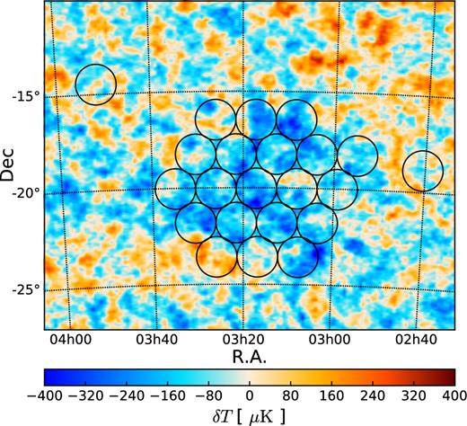
The 2CSz survey geometry. Superimposed on the Planck SMICA map of the CMB Cold Spot are circles representing the 22 3 deg² galaxy redshift fields observed using AAT 2dF+AAOmega. 20 of these fields lie within a 5° radius of the Cold Spot centre.

The imaging basis for this spectroscopic survey was the VLT Survey Telescope (VST) ATLAS (Shanks et al. 2015), an ongoing ∼4700 deg²ugriz survey at high galactic latitude over the two sub-areas in the North and South Galactic Caps (NGC and SGC, respectively), the latter of which includes the Cold Spot region. VST ATLAS reaches an i-band 5σ depth of 22.0 AB mag for point sources and has a median i-band seeing of 0.81 arcsec, allowing clean star–galaxy classification to our magnitude limit. The main selection criterion was to select extended sources with i_{Kron, AB} ≤ 19.2, where Kron indicates a pseudo-total magnitude with the usual definition. Additional quality control cuts were applied to the data to ensure the removal of stars and spurious objects from the galaxy catalogue. Although the extended source classification removes most stars, an additional star–galaxy cut was applied (i_{Kron, AB} − i_{ap3, AB} < 0.1 × i_{Kron, AB} − 1.87), where i_{ap3, AB} denotes the magnitude corresponding to the flux within a 2 arcsec diameter aperture (cf. fig. 22 of Shanks et al. 2015). To reject spurious objects (e.g. ghosts around bright stars), sources without z-band detections were rejected, as were objects near Tycho-2 stars at radii calibrated to VST ghosts. Additionally, a cut of SKYRMS ≤ 0.2 ADU was applied to the rms of the sky measurement for each source in the catalogue to remove further artefacts. These cuts were validated with GAMA G23. All magnitudes were corrected for Galactic extinction (Planck Collaboration et al. XI 2014).

The spectroscopic survey was completed in 22 2dF fields with 20 covering the inner 5° radius of the Cold Spot. The survey footprint is shown in Fig. 1. 2dF covers a 3 deg² area with approximately 392 fibres, ∼25 of which were used as sky fibres. The number density of selected galaxies was 722 deg⁻², further randomly sampled down to ∼200 deg⁻² in order to provide sufficient targets to utilize all fibres. Many targets cannot be observed due to limitations in positioning of the fibres to avoid fibre collisions and to limit fibre crossings. This down-sampled target list was finally supplied to the 2dF fibre allocation system Configure.

The spectroscopic observations were carried out in visitor mode on 2015 November 16–18, during grey (Moon phase) conditions with typical seeing of ∼2.0 arcsec. We observed using AAOmega with the 580V and 385R gratings and the 5700 Å dichroic. This gives a resolution of R ∼ 1300 between 3700 and 8800 Å. Each field was observed with 3 × 15 min exposures; flats and an arc frame were also taken with each plate configuration. Fields observed at high airmass at the beginning and end of the night had additional 15 min exposures where possible. Dark and bias frames were taken during the day before and after each night.

Spectroscopic observations were reduced and combined using the 2dFdr pipeline (Croom, Saunders & Heald 2004; Sharp & Parkinson 2010). The data were corrected with the fibre flat and median sky subtracted. Dark frames were not ultimately used as on inspection they did not improve the data quality. The sky correction parameters used were throughput calibration using sky lines, iterative sky subtraction, telluric absorption correction and principal component analysis after normal sky subtraction. The resulting reduced spectra were then redshifted manually using the package runz (Colless et al. 2001; Saunders, Cannon & Sutherland 2004). Redshifts were ranked in quality from 5 (template quality), 4 (excellent), 3 (good), 2 (possible) and 1 (unknown redshift). Only redshifts of quality 3 or greater were used in the final science catalogue. Typically, excellent quality redshifts had multiple strong spectra features (e.g. Hα, [O ii] and Ca ii H&K lines) and good redshifts contained at least one unambiguous feature. Overall, the redshift success rate was approximately 89 per cent ranging from 71 to 97 per cent; typically the success rate is a strong function of the phase and position of the Moon. The survey parameters are summarized in Table 1.

Table 1.

2CSz survey parameters.

Main selection	i ≤ 19.2
Area	66 deg2
Number of galaxiesa	6879
Completeness	89 per cent
Redshift range	0.0 ≤ z ≤ 0.5
Galactic coordinates (l, b)	(209, −57)

Note.^aGalaxies with redshift quality ≥3.

With an 89 per cent success rate, incompleteness will have only a small effect if redshift failures are random rather than systematic, and we modelled this with GAMA G23. To test what effect magnitude-dependent completeness could have on these results, we measured the completeness with magnitude for our survey, finding that completeness is ∼96 per cent for i_AB ≤ 18.2 and decreases to ∼82 per cent for 18.7 < i_AB ≤ 19.2. This magnitude-dependent completeness will bias the n(z) towards the redshift distribution of the brighter galaxies. To estimate the effect this has on the n(z), we weight the GAMA G23 n(z) with the completeness as a function of magnitude from 2CSz. Taking the ratio of the weighted and unweighted n(z), we obtain the completeness fraction as a function of redshift, f(z) ≈ 0.95 − 0.232z for z < 0.45. This linear modulation of the n(z) does not significantly affect the results but this analysis assumes that redshift failures depend only on the magnitude of the object and not the redshift. We do not apply a correction to the data as we do not believe this assumption holds (see Section 4.1).

3 RESULTS

3.1 Redshift distributions

The 2CSz redshift distribution of the ∼6879 quality >2 galaxies is shown in Fig. 2(a), along with the mean GAMA redshift distribution and a homogeneous model (Metcalfe et al. 2001). Comparison with the homogeneous model allows for under- and overdensities to be identified. Due to the sub-sampling of the spectroscopic survey, we normalized the n(z)’s to the galaxy number magnitude counts in the Cold Spot and G23 regions using an ATLAS iz band-merged catalogue. We found that the 75 deg² Cold Spot area was 16 ± 3 per cent underdense relative to the ∼1000 deg² around G23. We also found that the Cold Spot had a 7.4 ± 0.7 per cent number density deficit relative to a similarly large ∼1000 deg² region surrounding the Cold Spot whereas the G23 galaxy count was consistent with the SGC average over its full ∼2600 deg² area. Both the SGC number count and the mean galaxy density averaged over the 4 complete GAMA fields are in good agreement with the homogeneous model. To allow comparison with G23, we chose to normalize the Cold Spot observed n(z) by 7.4 per cent lower in total counts than both the homogeneous model and the G23 observed n(z), and this is what is shown in Fig. 2. Ignoring the large-scale gradient like this is certainly correct if it is a data artefact. But there is also a case to be made for it even if it is real since the Cold Spot is essentially a small-scale, ∼75 deg², feature rather than a ∼1000 deg² feature.

Figure 2.

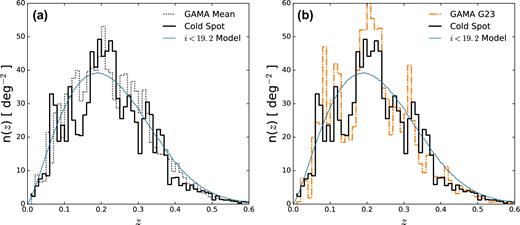
(a) The galaxy redshift distribution of the 2CSz (black). Also shown is the n(z) from the average of the four GAMA fields at RA ∼ 9, 12, 15 and 23 h (G23) at the same i_AB < 19.2 limit (grey dotted) and the homogeneous model of Metcalfe et al. (2001, blue). (b) The galaxy redshift distribution of the 2CSz (black). Also shown is the n(z) from the GAMA G23 field, at the same i_AB < 19.2 limit (yellow dot–dashed), and the same homogeneous model as in panel (a) (blue).

Here and throughout, field-field errors are used. These are based on a (2dF) field size of ∼3 deg².

The mean GAMA redshift distribution comes from the four GAMA fields, G23, G09, G12 and G15 selected with i_AB ≤ 19.2. The latter three r-limited fields were checked to be reasonably complete at the i_AB ≤ 19.2 limit for this analysis. The stacked GAMA redshift distribution fits well with the Metcalfe et al. (2001) homogeneous model for galaxies with i_AB ≤ 19.2. Fig. 2(a) shows indications of inhomogeneity in the Cold Spot sightline where we see evidence of an underdensity spanning 0.08 < z < 0.17 and there is also a hint of a smaller underdensity at 0.25 < z < 0.33. This would be consistent with the Szapudi et al. (2015) supervoid but we also see evidence for an overdensity at 0.17 < z < 0.25, apparently in conflict with the previous claim that the supervoid was centred in this range. Given the photometric redshift error, there may be no real contradiction between the data sets but their single void model does appear inconsistent with our spectroscopic data (see Section 4.2). Another underdensity is seen at 0.37 < z < 0.47 but systematic errors, such as spectroscopic incompleteness, become more important at this point (see Section 4.1).

3.2 Void model

In order to obtain the parameters of an underdensity and determine its ISW imprint, a void profile must be selected and fitted to the redshift distribution. Some previous work has used simple top-hat void models as the measured profile was dominated by photo-z error. In the case of our well-sampled spectroscopic survey, the structure of the void is important to the fitting and allows us to estimate the ISW imprint of any void. Following Kovács & García-Bellido (2016), we have chosen the Lambda Lemaître–Tolman–Bondi void profile described by a Gaussian potential (i.e. α = 0 in Finelli et al. 2016, equation 1), which will allow us to use the analytic expression for the ISW temperature profile given by these authors. This compensated void profile is described as

\begin{equation} \delta _{\rm m}(r) = \delta _0\ g(a) \left( 1 - \frac{2}{3}\,\frac{r^2}{r_0^2} \right) \exp \left(-\frac{r^2}{r_0^2}\right), \end{equation}

(1)

where δ_m(r) is the matter density contrast at radius r from the void centre, δ₀ is the matter density contrast at the void centre, g(a) is the growth factor at scalefactor, a, and r₀ is the void radius. As shown by Finelli et al. (2016), the ISW imprint of a void described by equation (1) can be calculated using

\begin{eqnarray} \frac{\delta T}{T}(\theta )& \approx & \frac{3 \sqrt{\pi }}{22} \frac{H(z_0) \Omega _{\Lambda } F_4(-\Omega _{\Lambda }/\Omega _{M}(1+z_0)^3)}{H_0 (1+z_0)^4 F_1(-\Omega _{\Lambda }/\Omega _{M})} \nonumber\\ &\times & \left( 1\!+\!{\rm erf}\left(\frac{z_0}{H(z_0) r_0}\right) \right) \delta _0 (H_0 r_0)^3 \exp \left[-\frac{r^2(z_0)}{r_0^2}\theta ^2\right]\!, \end{eqnarray}

(2)

where |$\frac{\delta T}{T}(\theta )$| is the ISW temperature imprint at angle θ away from the centre of the void and z₀ is the central redshift of the void. F₁ and F₄ are described by equations (3) and (4), respectively, where ₂F₁ is the hypergeometric function,

\begin{equation} F_1 = \ {}_2 F_1\ \left[1,\frac{1}{3},\frac{11}{6},\frac{-\Omega _{\Lambda }a^3}{\Omega _M}\right], \end{equation}

(3)

\begin{equation} F_4 = \ {}_2 F_1\ \left[2,\frac{4}{3},\frac{17}{6},\frac{-\Omega _{\Lambda }a^3}{\Omega _M}\right]. \end{equation}

(4)

Finelli et al. (2016) also give an expression for the Rees–Sciama effect (Rees & Sciama 1968), the second-order ISW effect. As the Rees–Sciama effect is sub-dominant to the ISW effect at the scale of the Cold Spot at low redshift in the standard cosmology (Cai et al. 2010), we will neglect its contribution in our calculations.

3.3 Perturbation fitting in the Cold Spot

In order to estimate the ISW imprint of the observed inhomogeneities, we have fitted the redshift distribution with compensated perturbations with the profile given by equation (1). Although our spectroscopic survey has 3D information, we pursue this 1D analysis to mimic the void finding used in past photo-z analyses, so the same large underdensities are selected. In order to do this, it was first necessary to transform the n(z) to the matter density contrast, δ_m(z), done by first converting to the galaxy density contrast, δ_g(z), and then dividing by the galaxy bias, b_g. These transformations are shown as

\begin{equation} \delta _{\rm g}(z) = \frac{n(z)}{n_{\mathrm{model}}(z)}-1 \end{equation}

(5)

\begin{equation} \delta _{\rm m}(z) = \frac{\delta _{\rm g}(z)}{b_{\rm g}}, \end{equation}

(6)

where n_model(z) is the predicted redshift distribution from the homogeneous model (Metcalfe et al. 2001). Since the magnitude limits for the 2CSz and G23 galaxies are the same, the bias for both samples can be estimated from the GAMA G23 correlation function, obtaining a linear bias of b_g = 1.35. Although simplistic, this linear bias assumption is accurate enough for the large scales of interest here.

Fig. 3(a) shows the matter density contrast for the 2CSz survey, assuming field-field errors. A number of features can be seen in Fig. 3(a). At the lowest redshifts (z < 0.06), the ‘Local Hole’ can be seen as a ∼25 per cent underdensity. This is well studied in the literature and seems to extend across the SGC (e.g. Whitbourn & Shanks 2014). At z = 0.06, there is an overdensity separating the ‘Local Hole’ from a ∼40 per cent underdensity that extends to z = 0.17. Another peak in the distribution is followed by two underdensities (z = 0.23, 0.25 and 0.3, respectively). Lastly, there is a clear break at z = 0.38 and a ∼30 per cent underdensity extending to z = 0.5 where it converges towards the homogeneous model. This feature may be due to redshift-dependent incompleteness as we will discuss later (see Section 4.1).

Figure 3.

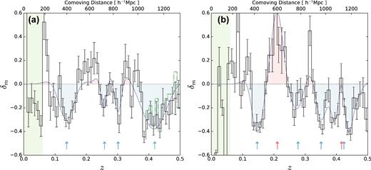
(a) The matter density contrast for 2CSz (black histogram), the best-fitting void models (dark blue) and the ‘Local Hole’ extent (green); modelled underdensities are filled in blue and overdensities in red. The dashed line shows the result at z > 0.38 when only 2dF fields with >90 per cent redshift success rate are used. Arrows indicate the centre of each fitted underdensity (blue) and overdensity (red). (b) The mass density contrast for the GAMA G23 with symbols as in panel (a).

In order to fit the redshift distributions in an unbiased way, we have adopted an iterative fitting procedure that minimizes the necessary complexity of any fit, quantified with the Akaike information criterion (AIC; e.g. Porciani & Norberg 2006). The AIC statistic takes into account the improvement in the fit of a more complex model but additionally penalizes it for this increased complexity. We use the AIC statistic specifically because it can be corrected in the case when the number of data points is not much larger than the number of parameters. We have fitted individual underdensities, δ_m(r), with 3D perturbations described by equation (1), averaged over the 5 deg radius of 2CSz. In order to describe the features seen in Fig. 3, we model the line of sight n(z) as a combination of perturbations. The fitting assumes that the void is centred on the Cold Spot. The whole redshift range was fitted simultaneously, with the ‘Local Hole’, at z ≤ 0.0625 excluded from the fit as it is not unique to the Cold Spot. We do not believe this will affect our results as there is a clear overdensity, which appears to be a wall, separating the Local Hole and the lowest redshift void we consider. Our iterative method initially assumed N perturbations seeded with random parameters and fitted them to the data. Fitting was carried out with a Levenberg–Marquardt algorithm and quoted errors are standard errors calculated from the covariance matrix. Iterating over new random values and fitting, we converge on the best-fitting parameters for N perturbations. The best fits for each value of N were then compared via the corrected AIC statistic, the minimum of which gave the optimum fit and the relative likelihood allowed for other values of N to be rejected if significantly poorer. The corrected AIC statistic is given by equation (7) (Porciani & Norberg 2006), where k is the number of parameters being fit, N_data is the number of data points and |$\hat{L}$| is the maximized likelihood function,

\begin{eqnarray} \mathrm{AIC} & = & 2k - 2 {\rm ln}(\hat{L}) + \frac{2k(k+1)}{N_{\mathrm{data}}-k-1} \nonumber\\ & = & 2k + \chi ^2 + \frac{2k(k+1)}{N_{\mathrm{data}}-k-1}. \end{eqnarray}

(7)

The second line of equation (7) holds in the case of normally distributed residuals. The relative probability of one model over another with a greater AIC value is given by the Akaike weights (equation 8), where AIC_min is the minimum AIC, ΔAIC_i = AIC_i − AIC_min and k_max is the maximum k considered,

\begin{equation} w_i = \frac{ {\rm e}^{-\Delta \mathrm{AIC}_i/2}}{\sum _{k=1}^{k_{\mathrm{max}}}{\rm e}^{-\Delta \mathrm{AIC}_k/2}}. \end{equation}

(8)

Hence, a p = 0.05 rejection of the weaker model corresponds to a ΔAIC ∼ 6, and we shall adopt ΔAIC = 6 as a threshold for rejecting models over the best fit. More complex models were considered until one was rejected over a simpler model.

This analysis suffers from degeneracies in that we cannot discern the difference between two voids and a wide void with an interior, narrow overdensity. For this reason, the fitting ranges of parameters were restricted in a range to provide sensible fits. Specifically, we restricted the void radius to be between 50 and 150 h⁻¹ Mpc and the central density contrast was constrained to lie in the physical range, δ₀ ≥ −1. Parameters at the radius limits were individually re-fitted. Fits were also rejected that had perturbations at the very edges of the fitting range, i.e. z₀ < z_min + 0.01 or z₀ > z_max − 0.01. Additionally, the compensated profile we have adopted cannot describe sharp narrow underdensities as they are averaged out in the survey field; however, the purpose of this analysis is to detect large voids and this places upper limits on ISW contributions. We have allowed overdensities to be fitted with the perturbation described by equation (1), but as this profile was derived for voids, the resulting δT values should be treated with caution. The minimum AIC values for each value of N perturbations are shown in Table 2. The resulting best fits are shown in Fig. 3. For the Cold Spot, the iterative procedure selected N = 4 perturbations as the best fit (all underdensities) to give the fits summarized in Table 3. The AIC test does not strongly reject the N = 5 solution but we note that the difference between the models is only in the fitting of the z ∼ 0.42 void with one profile or two and the resulting total δT differs by just 2.7 μK, which is not significant.

Table 2.

The minimum AIC values for each value of N perturbations for the Cold Spot and G23. k is the number of free parameters. The minimum AIC values for each field are shown in parentheses, these are the best fits.

N	k	AICmin
		Cold Spot	G23
1	3	248.85	441.97
2	6	147.17	240.14
3	9	131.65	197.66
4	12	(123.91)	154.64
5	15	125.18	151.07
6	18	132.33	(141.45)
7	21	–	149.86

Table 3.

Best-fitting 3D ΛLTB parameters for compensated perturbations (equation 1) estimated from the Cold Spot and GAMA G23 density contrast profiles in Fig. 3. The central temperature decrement, δT, predicted from the ISW effect is also given.

	z0	r0 (h−1 Mpc)	δ0	δT(θ = 0) (μK)
Cold Spot
	0.14±0.007	119±35	−0.34±0.08	−6.25±5.7
	0.26±0.004	50±13	−0.87±0.12	−1.02±0.8
	0.30±0.004	59±17	−1.00+0.72	−1.80±2.1
	0.42±0.008	168±33	−0.62±0.16	−22.6±14.7
G23
	0.15±0.004	82±33	−0.49±0.17	−2.92±3.7
	0.21±0.006	88±21	+0.89±0.35	+6.09±5.1
	0.28±0.007	85±29	−0.36±0.24	−2.06±2.6
	0.35±0.006	74±22	−1.00+0.10	−3.40±3.1
	0.42±0.005	150±20	−0.63±0.13	−16.1±7.4
	0.42±0.002	50±5	+4.16±1.6	+3.96±2.0

3.4 Perturbation fitting in GAMA G23

As noted above, we originally planned to use GAMA G23 as a control field but analysis showed that even on 50 deg² scales there was sufficient sample variance to merit using a model that we validated with the stacked i_AB ≤ 19.2 n(z) from all four GAMA fields with a combined area of ∼240 deg². Indeed, Fig. 2(b) shows that upon comparison the Cold Spot redshift distribution bears remarkable similarity with G23 in the underdensities at z ∼ 0.15, 0.3 and 0.4. In particular, the significant underdensity 0.35 < z < 0.5 that occurs in both fields could point to a selection effect in the survey. However, the mean GAMA redshift distribution shown in Fig. 2(a) shows little evidence for this. It also raises the question of whether or not some of these features could be coherent between G23 and the Cold Spot. Certainly, at the lowest redshifts of z < 0.05, the underdensity is consistent with the ‘Local Hole’ that spans the SGC (Whitbourn & Shanks 2014). In Section 4.3, we shall use the 2dF Galaxy Redshift Survey (2dFGRS; Colless et al. 2001), whose Southern Strip spans the SGC between GAMA G23 and the Cold Spot, to check if this apparent coherence is real or accidental.

Meanwhile, the n(z) similarities open up the possibility of G23 still acting as a control field because it does not show a CMB Cold Spot. Therefore, due to the similarities in the redshift distributions of G23 and 2CSz, we have fitted the density contrast in the same way as the Cold Spot as shown in Fig. 3(b). The parameters of the best fit are summarized in Table 3 with N = 6 perturbations selected (see Table 2), including four underdensities and two overdensities. We note that the highest redshift feature has been fitted with an underdensity with an interior, narrower overdensity that together fit the two z > 0.37 underdensities seen in Fig. 3(b). The fitting procedure selects this over two underdensities because the underdensities are sharp and the density profile provides a poor fit individually. As we will discuss in Section 4.1, we believe these features are affected by systematics and therefore we did not re-fit them.

4 DISCUSSION

We have detected three large underdensities along the CMB Cold Spot sightline, the largest with radius r₀ = 119 ± 35 h⁻¹ Mpc centred at z₀ = 0.14 with a central density contrast of δ₀ = −0.34. This supervoid is smaller but more underdense than that proposed by Szapudi et al. (2015), which has r₀ ∼ 220 h⁻¹ Mpc and δ_g = −0.25. The Szapudi et al. (2015) void also has a higher central redshift at z ∼ 0.22 and may include the other 2CSz voids at z₀ = 0.26 and 0.30 (see Table 3), seen as a single supervoid due to the photo-z errors. Kovács & García-Bellido (2016) drew upon additional data sets to suggest that the proposed supervoid extended back to zero redshift with radius 500 h⁻¹ Mpc and with a smaller 195 h⁻¹ Mpc radius in the angular direction. From equation (2), we estimate the central temperature decrement due to our z = 0.14 void at − 6.25 ± 5.7 μK, small compared to some previous work (Kovács & García-Bellido 2016), as expected due to the strong relationship between void radius and its ISW imprint. The combined ISW imprint of the three Cold Spot voids is − 9.1 ± 6.1 μK and even adding the fourth questionable void this rises to just − 31.7 ± 15.9 μK. As we will discuss in Section 4.1, we believe the z = 0.42 void is exaggerated by systematics. We also note that these estimates of the ISW imprint depend on the chosen void density profile used in the fitting process. Although the profile used here (equation 1) is not unique, it is at least representative of what previous studies have done and allows for direct comparison with literature (e.g. Finelli et al. 2016; Kovács & García-Bellido 2016).

The strongest evidence against an ISW explanation for the Cold Spot that may arise from our results is due to the similarity in the n(z) between GAMA G23 and the Cold Spot. Despite this, G23 has no CMB Cold Spot. Indeed, the predicted central ISW decrement for G23 from summing the contributions in Table 3 (excluding the features at z > 0.4) is − 3.6 ± 7.5 μK, statistically consistent with the − 9.1 ± 6.1 μK predicted similarly for the Cold Spot. The predicted central ISW decrement for G23 is also consistent with that of the Cold Spot, even if no features in Table 3 are excluded. However, the CMB in the G23 sightline shows only a small central temperature decrement of − 15.4 ± 0.3 μK, some ∼10 times lower than for the Cold Spot. Thus, the similarity in the large-scale structure between G23 and the Cold Spot fields forms a further qualitative argument against foreground voids playing any significant role in explaining the Cold Spot. On this evidence alone the detected void cannot explain the CMB Cold Spot because a similar void in G23 has no such effect.

4.1 The reality of the z = 0.42 void

In the Cold Spot n(z), an apparent, relatively strong, void can be seen at 0.37 < z < 0.5 but we have already noted that this is in a range where not only are the statistics poorer but where we know that magnitude-dependent incompleteness becomes more important. The similarity of this feature with the 0.34 < z < 0.5 underdensities in G23 suggests that there may be some sort of selection effect or systematic that we will now investigate.

We therefore test the reality of this void in Fig. 4 where we compare the 2CSz δ_m(z) and the previous Bremer et al. (2010) VLT VIMOS δ_m(z) and see that an underdensity at z = 0.42 may also be detected in that data set, albeit at low ∼2σ significance. A lower bias of b = 1 has also been assumed here for the VIMOS δ_m(z) compared to b = 1.35 for 2CSz, on the grounds that the VIMOS galaxies are intrinsically fainter. This is consistent with results from the VVDS survey (Marinoni et al. 2005). We note that despite this apparent agreement the VLT VIMOS data probe a much smaller volume at this low-redshift end and therefore would have large sample variance.

Figure 4.

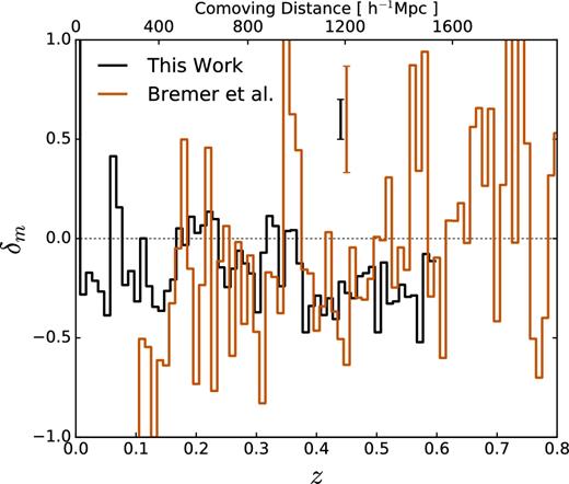
The 2CSz δ(z) (black) compared with VLT VIMOS (Bremer et al. 2010) δ(z) (orange) to test the reproducibility of the Cold Spot void at z = 0.42. Here a bias of b = 1.35 has been assumed for the 2dF δ(z) and a bias of b = 1 has been assumed for VLT VIMOS δ(z). Typical errors are plotted above the lines; Poisson errors are assumed for the VIMOS data.

The absence of this feature from the mean GAMA n(z) indicates that this feature cannot be intrinsic to the i_AB < 19.2 selection criteria. We instead suggest that it may be due to a systematic selection effect. Although the other GAMA fields are apparently unaffected by this systematic, this may be explained by the Cold Spot (and G23) data having slightly lower S/N due to somewhat shorter 2dF exposure times and redshift success rate, namely Cold Spot (45 min, 89.0 per cent), G23 (30–50 min, 94.1 per cent) versus the other three equatorial GAMA fields used here (50–60 min, 98.5 per cent). 2CSz was also conducted in grey time, which will further reduce the S/N with respect to GAMA. The lower S/N ratio will increase spectroscopic incompleteness, and we note that the 4000 Å break and Ca ii H&K absorption lines transition though the dichroic over this redshift range while the Hα emission line also leaves the red arm of the spectrograph. It is possible that these two effects make accurate redshifting more difficult over this redshift range and would create an apparent underdensity. To test this, we split 2CSz into pointings with high and low spectroscopic success rate, with half having a success rate greater than 90 per cent and half with less. The result of this is shown for z ≥ 0.38 in Fig. 3(a) by the dashed histogram. All fitting used the full data set. The success rate of the 2dF field strongly affects the depth of the z = 0.42 void indicating that it is affected by systematic incompleteness.

Also, at z > 0.4, small differences in the homogeneous model will lead to large differences in the derived δ_m(z). To investigate whether the model n(z) could be overpredicting the galaxy density at the higher redshifts creating spurious underdensities, we have explored a model n(z) constructed from random catalogues built for the GAMA survey (Farrow et al. 2015) and find that indeed this different model n(z) decreases the depth of the z = 0.42 void. When compared to the mean GAMA n(z) however this model n(z) appears to underpredict the galaxy density at higher redshift and therefore we do not replace our homogeneous model with the GAMA random catalogue constructed n(z). Whether the void seen by 2CSz in this z range is accentuated by such systematics or not does not matter for our main conclusion since even including this void's contribution the total ISW decrement from Table 3 is still only ∼ − 32 μK compared to the ∼ − 150 μK needed to explain the Cold Spot.

Additionally, we note that the bias of galaxies will not be constant throughout the redshift range as assumed. Because the survey is magnitude limited, the galaxies at the high-redshift end of the survey will be brighter than the low-redshift end. The brighter 2CSz galaxies at z = 0.42 may actually be as large as b ∼ 2 (e.g. Zehavi et al. 2011), and increasing the bias would linearly decrease the depth of the void δ₀ (by equation 6) and hence its ISW imprint.

Together these arguments cast doubt on the existence of the z = 0.42 void, and for this reason we neglect it in our conclusions. A sample of galaxies with a magnitude limit intermediate between that of 2CSz and Bremer et al. (2010) is needed to determine finally the status of the z = 0.42 void.

4.2 Photo-z and spectroscopic n(z)

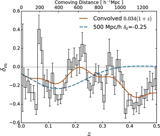
In order to assess why the spectroscopic 2CSz survey results apparently differ from the photometric redshift survey of Kovács & García-Bellido (2016), we convolved the 2CSz spectroscopic redshift distribution with an estimated error of 0.034(1 + z) photo-z error, which is the quoted photo-z error from Szapudi et al. (2015). Kovács & García-Bellido (2016) used 2MPZ with a very small photo-z error of 0.015(1 + z), but the 2MPZ sample is limited by low number densities at higher redshifts so we do not compare to this directly.

The resulting model δ_m(z) is shown in Fig. 5 where we see that there is limited consistency with the model result of Kovács & García-Bellido (2016) with r₀ = 500 h⁻¹ Mpc and δ₀ = −0.25 when convolved with a photo-z error. The main source of disagreement is the lack of an underdensity at z ∼ 0.2 in 2CSz, which seems difficult to reconcile with the model void but we note that at z > 0.15 the 2MPZ data are consistent with no underdensity due to a large uncertainty. While our data are not consistent with an r₀ = 500 h⁻¹ Mpc void, we believe it is consistent with the photo-z data.

Figure 5.

The 2CSz δ_m(z) (black), the 2CSz δ_m(z) convolved with the photo-z error of the Pan-STARRS data of Szapudi et al. (2015, orange) and compared to the fitted δ_m(z) model of Kovács & García-Bellido (2016, blue).

When we compare our predicted ISW central decrement to previous work, we see some consistency. With the 3-void model of the Cold Spot line of sight, the combined temperature decrement is − 9.1 ± 6.1 μK, which is consistent with the ∼ − 20 μK of Szapudi et al. (2015) but not with the ∼ − 40 μK of Kovács & García-Bellido (2016). One could argue that the 4-void model at − 31.7 ± 16.0 μK is consistent with Kovács & García-Bellido (2016) values, but |${\sim } \frac{2}{3}$| of that decrement is due to the z = 0.42 void that is likely to be contaminated by systematic effects as discussed previously. Additionally, the void of Kovács & García-Bellido (2016) did not extend to z > 0.4 and it is beyond the range of the 2MPZ data.

4.3 A coherent SGC galaxy distribution?

We have already discussed the important question of the normalization of the Cold Spot n(z). Both G23 and the Cold Spot areas are contained in the Local Hole underdensity known to extend at least to z = 0.06 across the SGC. Moreover, we have noted that the galaxy count in the 5° radius Cold Spot area is ∼16 per cent underdense relative to G23 and the rest of the SGC at our i_AB < 19.2 limit. When compared to a surrounding ∼1000 deg² area, the 5° core of the Cold Spot is 7.4 per cent underdense. The Cold Spot area therefore appears to exist in an environment exhibiting a significant global gradient stretching across the SGC. Finally, we have noted the similarity of the 2CSz and GAMA G23 redshift distributions that again may suggest evidence for coherent structure extending between them.

To investigate further this possibility, we now exploit the 2dFGRS (Colless et al. 2001) that spans the SGC between GAMA G23 and the Cold Spot at −35° < Dec. < −25° (see Fig. 6). With a magnitude limit b_J(∼g) ≤ 19.6, 2dFGRS is shallower than the i_AB ≤ 19.2 surveys so only probes the low-z structures but has a large area. Busswell et al. (2004) show the redshift distribution of the 2dFGRS survey in the SGC in their fig. 14 (also shown in fig. 13 of Norberg et al. 2002). The distribution shows peaks at z = 0.06, 0.11 and 0.21, which are very similar to those shown in 2CSz and roughly similar to those shown in G23. We have attempted to track these features across 2dFGRS to see if they do in fact span the sky between G23 and 2CSz. When we split 2dFGRS by RA as in Fig. 7, we generally see coherence in that at z < 0.06 we consistently see underdensity in this range. This is the ‘Local Hole’ of Whitbourn & Shanks (2014, see their fig. 2b), which covers ∼3500 deg² of the SGC (the 6dFGS SGC area marked in orange in their fig. 1 with coordinate ranges given in their table 3). Based on the 0.06 < z < 0.11 void seen in the 2dFGRS n(z) shown in fig. 14 of Busswell et al. (2004), these authors have speculated that the void runs to z ∼ 0.1. In passing, we note that the ∼8 per cent gradient between the regions surrounding G23 and the Cold Spot may represent Local Hole sub-structure.

Figure 6.

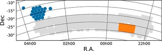
The position of the 2dFGRS SGC strip (grey) relative to the 2CSz 2dF fields (blue) and the GAMA G23 area (orange).

Figure 7.

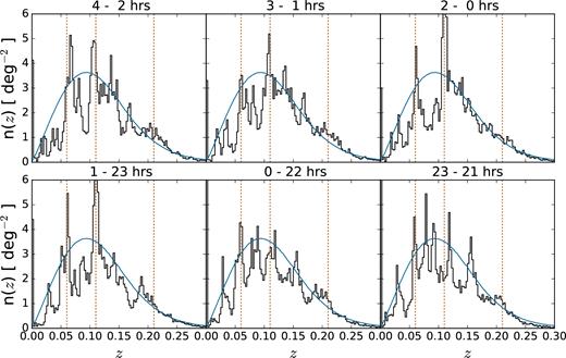
The 2dFGRS SGC galaxy redshift distributions, n(z), in overlapping 2 h ranges of RA at Dec. ∼−30 ± 5 deg (black). The homogeneous model prediction of Metcalfe et al. (2001) to the 2dF limit of b_j = 19.6 is plotted (blue). The redshifts corresponding to the peaks in the average 2dFGRS n(z) at z = 0.06, 0.11 and 0.21 are marked (orange dashed lines).

In Fig. 7, we see that the eastern half of 2dFGRS (0 < RA < 4 h) more clearly exhibits the peaks at z = 0.06 and 0.11 (with intervening underdensity) than does the range at 21 < RA < 0 h. We have checked that restricting 2dFGRS to the G23 area produces very good agreement in δ_m(z) out to z < 0.25. More speculatively, even the z = 0.21 peak may be seen in at least some of the RA ranges. If so, this possible coherence may also explain why 2CSz and G23 have such similar n(z) distributions. However, in the 23 < RA <1 h and 0 < RA < 2 h ranges, the feature at z = 0.21 is less obvious and perhaps argues against coherence extending to z ∼ 0.2. This would leave the similarity of the 2CSz and G23 n(z)’s at 0.1 < z < 0.2 appearing accidental. We note that the absence of these structures from the NGC 2dFGRS survey (cf. figs 13 and 14 of Busswell et al. 2004) makes systematic effects unlikely as the cause.

How likely is it, in the standard cosmological model, that coherent structure extends out to z < 0.2 across the 2dFGRS SGC strip? We assume an ∼1000 deg² area for 2dFGRS SGC and a power-law correlation function, ξ(s) = (s/s₀)^−γ, with s₀ ∼ 6.92 h⁻¹ Mpc and γ ∼ 1.51 for s < 50 h⁻¹ Mpc, as measured for 2dFGRS by Hawkins et al. (2003). The variance, |$\sigma _N^2$|⁠, of galaxy numbers, N, around average |$\skew3\bar{N}$| in a volume, V, where the galaxy space density, n (=N/V), is (e.g. Peebles 1980)

\begin{equation} \sigma _N^2 =\langle (N-\skew3\bar{N})^2\rangle =\skew3\bar{N}+n^2\int _V\xi (s_{12}){\rm d}V_1{\rm d}V_2, \end{equation}

(9)

implying |$\sigma _N\sim 20\times \sqrt{\skew3\bar{N}}$|⁠. Given that |$\skew3\bar{N}\sim 140\,000$| galaxies in the 2dFGRS SGC volume, a nominal 10 per cent underdensity (or overdensity) across 2dFGRS SGC even out to z ∼ 0.2 would amount to a ∼1.9σ fluctuation. On the same assumptions, a similar over- or underdensity out to z = 0.1 would represent a significance of ∼1.3σ. Now, these may be taken as a rough measure of the significance of coherence in a survey modelled by some of its z range being 10 per cent overdense and the rest being 10 per cent underdense. So at ∼1.3σ–1.9σ, we conclude that galaxy clustering coherence across 2dFGRS SGC can plausibly explain the 2CSz–G23 coherence out to z ∼ 0.1 and more speculatively to z ∼ 0.2. However, the observational evidence for coherence at z ∼ 0.2 is mixed.

4.4 Origin of the CMB Cold Spot

As noted in Section 1, several authors have calculated the significance of the Cold Spot with respect to the coldest spots in CMB sky simulations (e.g. Nadathur et al. 2014; Planck Collaboration et al. XVI 2016b). The significances are typically at the ∼1 per cent level. As shown by these authors, the significance of the Cold Spot in the standard cosmology comes not from the central temperature but from the temperature profile seen in Fig. 8 that closely matches the compensated SMHW that was originally used to detect it (Vielva et al. 2004). On this basis when assessing what impact the detected voids have on the significance of the Cold Spot, we have to go beyond central temperature and look at the significance of the SMHW filtered temperature subtracted for the detected voids. This removes the ISW imprinted signal and assesses the significance of the residual primordial profile. Following Naidoo et al. (2016), subtracting our best 3-void (i.e. the voids with z₀ < 0.4 in Table 3) model, ISW contribution would reduce the significance of the Cold Spot only slightly, typically to ∼1.9 per cent (Naidoo et al. 2016), i.e. only 1 in ∼50 ΛCDM Universes would produce such a feature by chance. Fig. 8 shows the ISW imprints of the 3- and 4-void models and the measured CMB Cold Spot temperature profile. This significance would be reduced if our 4-void model was trusted but, as previously argued, the void at z = 0.42 may be unduly affected by systematics.

Figure 8.

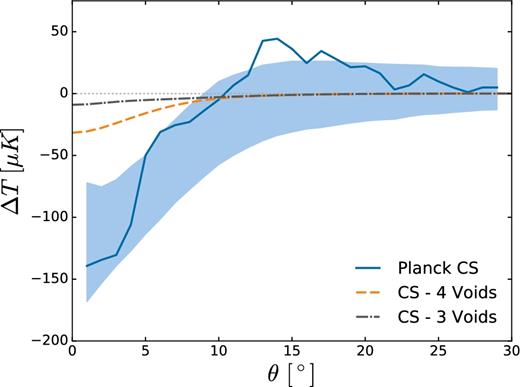
The Cold Spot temperature profile (Planck Collaboration et al. XVI 2016b, blue line) and the ISW imprints of the 3- and 4-void models (grey dot–dashed and yellow dashed, respectively) fitted to the Cold Spot region. The void temperature profiles from Table 3 have been summed and the result fitted to equation 3 of Naidoo et al. (2016). The shaded region (light blue) is the 68 per cent confidence interval from the coldest spots identified in Gaussian simulations (see fig. 6 of Nadathur et al. 2014).

Kovács & García-Bellido (2016) claimed that the Cold Spot supervoid is an elongated supervoid at z = 0.14 with r₀ = 500 h⁻¹ Mpc in the redshift direction and r₀ = 195 h⁻¹ Mpc in the angular direction with δ₀ = −0.25. The ISW effect on the central decrement is estimated to be a reduction of ∼ 40 μK. At the central redshift of z = 0.14, this supervoid would extend 27|$_{.}^{\circ}$|5 on the sky. We note that the 2dFGRS SGC strip covers the area to the South of the Cold Spot. In the 2 h < RA < 4 h range, all of this RA bin is within 27|$_{.}^{\circ}$|5 of the Cold Spot. Fig. 7 shows that although there is a 2dFGRS void at z = 0.08 within the supervoid redshift range, the peak at z = 0.11 and plateau out to z = 0.15 are near the claimed z = 0.14 centre of the supervoid; there seems little evidence of a void at 0.1 < z < 0.25 in this 2dFGRS 2 h < RA < 4 h range. The z = 0.2 peak may still be present indicating that there may be an underdensity at 0.15 < z < 0.2. So at least in the direction South of the Cold Spot, evidence for an extended simple void structure around its centre is again not present.

Various authors (e.g. Cai et al. 2014a,b; Kovács et al. 2017 and references therein) have also discussed the possibility of an enhanced ISW effect in voids being produced by modified gravity models. This has been done to explain observations where a larger-than-expected (2–4 times under ΛCDM) ISW-like signal has been found around voids (Granett et al. 2008; Cai et al. 2017); these results are however low significance. It may be speculated whether our 2CSz Cold Spot results may also be explained similarly. But again the similarity between the galaxy redshift distributions in 2CSz and the G23 control field tends to argue against this possibility. If some modified gravity model did give an enhanced ISW effect to explain the Cold Spot, then why is there no similar Cold Spot seen in the G23 line of sight? This argument should be tempered with the facts that, first, the n(z) agreement between the Cold Spot and G23 is inexact given that the n(z) peak at z = 0.21 is more pronounced in G23. This difference is reflected in the predicted ISW decrements, −9.1 ± 6.1 and − 3.6 ± 7.5 μK for the Cold Spot and G23, respectively. Secondly, the n(z)’s used to construct the δ_m(z)’s were normalized with respect to their surroundings and so do not contain all the information of the largest scale fluctuations. As discussed previously, the region surrounding the Cold Spot is underdense with respect to the region surrounding G23 by ∼8 per cent so the two fields are not exactly equivalent and the structures detected in this analysis are embedded in different large-scale potentials. This could have an effect on the Cold Spot ISW imprint, but likely at larger scales than the 5° radius feature we have mainly investigated here. One could argue that the alignment of the CMB Cold Spot and the large z = 0.14 void implies a causal link though the improbability of alignment but voids of this scale are not expected to be unique (Nadathur et al. 2014; Kovács et al. 2017) and our search was not blind nor the only attempt to detect for a void.

If not explained by a ΛCDM ISW effect, the Cold Spot could have more exotic primordial origins. If it is a non-Gaussian feature, then explanations would then include either the presence in the early universe of topological defects such as textures (Cruz et al. 2007) or inhomogeneous re-heating associated with non-standard inflation (Bueno Sánchez 2014). Another explanation could be that the Cold Spot is the remnant of a collision between our Universe and another ‘bubble’ universe during an early inflationary phase (Chang, Kleban & Levi 2009; Larjo & Levi 2010). It must be borne in mind that even without a supervoid the Cold Spot may still be caused by an unlikely statistical fluctuation in the standard (Gaussian) ΛCDM cosmology.

To conclude, based on the arguments and caveats above, we have ruled out the existence of a void at which could imprint the majority of the CMB Cold Spot via a ΛCDM ISW effect. The predicted decrement is consistent with some previous studies (Szapudi et al. 2015), although certainly at the low end of literature values. We have additionally placed powerful constraints on any non-standard ISW-like effect that must now show how voids, apparently unremarkable on 5° scales, can imprint the unique CMB Cold Spot. The presence of the detected voids only slightly relaxes the significance of the primordial residual of the CMB Cold Spot in standard cosmology to approximately 1 in 50, tilting the balance towards a primordial and also possibly non-Gaussian origin. But at this level of significance clearly any exotic explanation will have to look for further evidence beyond the Cold Spot temperature profile.

5 CONCLUSIONS

We have conducted a spectroscopic redshift survey of the CMB Cold Spot core in order to test claims from photo-z analyses for the existence of a large low-z void that could be of sufficient scale and rarity to explain the CMB Cold Spot.

• We have detected a 119 h⁻¹ Mpc, δ_g = −0.34 underdensity at z = 0.14. This underdensity is much less extended than found in photo-z analyses in the literature but is more underdense. The estimated ΛCDM ISW effect from this void is estimated at − 6.25 μK, much too small to explain the CMB Cold Spot.

• Two further small underdensities were observed at z = 0.26 and 0.30. The effect of these voids is even smaller than the z = 0.14 void.

• A further candidate void was detected at z = 0.42, although we conclude that this is most likely due to redshift incompleteness in the survey. Even if real this void would still not explain the CMB Cold Spot.

• Without detailed calculation, we have shown that the rarity of this void is not sufficient to motivate it as the cause of the CMB Cold Spot because of the similarity with GAMA G23. The comparability of underdensities at z ∼ 0.4 between G23 and the Cold Spot again means that even if the z = 0.42 void in the Cold Spot was not a systematic effect, it is not unique enough to suggest an effect beyond standard cosmology.

• Combining our data with previous work (Bremer et al. 2010), the presence of a very large void that can explain the CMB Cold Spot can be excluded up to z ∼ 1, beyond which the ISW effect becomes significantly reduced as the effect of the Cosmological Constant is diluted.

• The similarity between the 2CSz and G23 n(z) distributions may have some explanation in the similar n(z) seen in the 2dFGRS SGC strip that spans ∼60° between these sightlines. This includes the ‘Local Hole’ at z < 0.06 but may also include further structures out to z ∼ 0.2.

Our 2CSz results therefore argue against a supervoid explaining a significant fraction of the Cold Spot via the ISW effect. This suggests a primordial origin for the Cold Spot, either from an unlikely fluctuation in the standard cosmology or as a feature produced by non-Gaussian conditions in the early Universe.

Acknowledgements

We thank N. Metcalfe, K. Naidoo and A. J. Smith for valuable discussions. We acknowledge the GAMA team for providing survey data in advance of publication. Based on data products from observations made with ESO Telescopes at the La Silla Paranal Observatory under programme ID 177.A-3011(A,B,C,D,E,F). We further thank OPTICON and the staff at the Australian Astronomical Observatory for their observing support at the AAT. GAMA is a joint European-Australasian project based around a spectroscopic campaign using the Anglo-Australian Telescope. The GAMA input catalogue is based on data taken from the Sloan Digital Sky Survey and the UKIRT Infrared Deep Sky Survey. Complementary imaging of the GAMA regions is being obtained by a number of independent survey programmes including GALEX MIS, VST KiDS, VISTA VIKING, WISE, Herschel-ATLAS, GMRT and ASKAP providing UV-to-radio coverage. GAMA is funded by the STFC (UK), the ARC (Australia), the AAO and the participating institutions. The GAMA website is http://www.gama-survey.org/. The G23 GAMA data set is in part based on observations made with ESO Telescopes at the La Silla Paranal Observatory under programme ID 177.A-3016. PN acknowledges the support of the Royal Society, through the award of a University Research Fellowship and the European Research Council, through receipt of a Starting Grant (DEGAS-259586). RM, TS and PN acknowledge the support of the Science and Technology Facilities Council (ST/L00075X/1 and ST/L000541/1). MLPG acknowledges CONICYT-Chile grant FONDECYT 3160492.

1

The Galaxy And Mass Assembly (GAMA) survey (Driver et al. 2009, 2011) includes three equatorial fields at RA ∼ 9, 12 and 15 h, each covering about 60 deg², highly spectroscopically complete to r_AB < 19.8. There is also one SGC field (G23) covering 50 deg² similarly complete to i_AB = 19.2 (Liske et al. 2015).