Gamma-ray burst efficiency and possible physical processes shaping the early afterglow

Abstract

The discovery by Swift that a good fraction of gamma-ray bursts (GRBs) have a slowly decaying X-ray afterglow phase led to the suggestion that energy injection into the blast wave takes place several hundred seconds after the burst. This implies that right after the burst the kinetic energy of the blast wave was very low and in turn the efficiency of production of γ-rays during the burst was extremely high, rendering the internal shocks model unlikely. We re-examine the estimates of kinetic energy in GRB afterglows and show that the efficiency of converting the kinetic energy into γ-rays is moderate and does not challenge the standard internal shock model. We also examine several models, including in particular energy injection, suggested to interpret this slow decay phase. We show that with proper parameters, all these models give rise to a slow decline lasting several hours. However, even those models that fit all X-ray observations, and in particular the energy injection model, cannot account self-consistently for both the X-ray and the optical afterglows of well-monitored GRBs such as GRB 050319 and GRB 050401. We speculate about a possible alternative resolution of this puzzle.

radiation mechanisms: non-thermal, ISM: jets and outflows, gamma-rays: bursts, X-rays: general

1 INTRODUCTION

The X-ray telescope (XRT) onboard Swift has provided high-quality early X-ray afterglow light curves of many gamma-ray bursts (GRBs). One of the most remarkable and unexpected features discovered by Swift was that many of these X-ray afterglow light curves are distinguished by a slow decline – the flux F decreases with observer's time t as F∝t^[0,−0.8], lasting from a few hundred seconds to few hours (Campana et al. 2005; Cusumano et al. 2006; Nousek et al. 2005; Vaughan et al. 2006; de Pasquale et al. 2006). Such a phase is unexpected in the standard fireball model. A simple explanation is that the slow decline arises due to a significant energy injection (Nousek et al. 2005; Zhang et al. 2005; Granot & Kumar 2006; Panaitescu et al. 2006), as suggested previously (for baryon-rich injection, see Panaitescu, Mészáros & Rees 1998; Rees & Mészáros 1998; Kumar & Piran 2000; Sari & Mészáros 2000; Zhang & Mészáros 2002; Granot, Nakar & Piran 2003; for Poynting flux-dominated injection1, see Dai & Lu 1998a; Zhang & Mészáros 2001; Dai 2004. It has been argued that consequently the resulted GRB efficiency, i.e. the ratio of the energy emitted in γ-ray energy to the total energy (the sum of the γ-ray energy and the kinetic energy of the ejecta powering the afterglow), should be 90 per cent or higher. Some extreme assumptions are needed (Beloborodov 2000; Kobayashi & Sari 2001) to reach such a high efficiency within the framework of the standard internal shocks model (Paczynski & Xu 1994; Rees & Mészáros 1994; Kobayashi, Piran & Sari 1997; Sari & Piran 1997a,b; Daigne & Mochkovitch 1998; Piran 1999).

We re-examine this issue focusing on two critical aspects of the analysis. The estimate of the kinetic energy of the ejecta from the afterglow observations and in particular from the X-ray flux and the need of energy injection. We show in Section 2 that even for these Swift GRBs with long duration X-ray flattening the γ-ray conversion efficiency is high but not unreasonable.

We then turn to the puzzling slow decline seen in the first few hours of the X-ray afterglow. We explore in Section 3 several models that may give rise to slowly decaying X-ray afterglows. (i) Energy injection. (ii) A small ζ_e, in which only a small fraction, ζ_e≪ 1 of the electrons are accelerated to high energies and contribute to the radiation process. (iii) Evolving shock parameters, where the microscopic shock parameters ε_e and/or ε_B (the fraction of shock energy given to the magnetic filed) vary in time and are inversely proportional to the Lorentz factor of the ejecta. (iv) A very low-variable external density model, in which the number density of the medium is not only very low but it also a function of the radius. (v) Highly magnetized outflow where flattening might arise because of a slow conversion of the magnetic energy to kinetic energy of the external matter. We present in Section 3 analytical derivation as well as numerical calculations of the expected light curves in all these models except the last one. In Section 4, we compare the models to the observations of GRB 050319 and GRB 050401. We summarize our results and discuss their implications in Section 5. We conclude with a speculation on the nature of the solution to this puzzle.

2 IS THERE A GRB EFFICIENCY CRISIS?

One of the critical factors that characterize the emitting of a GRB is the energy conversion efficiency. The γ-ray efficiency is defined as

1

where E_γ is the isotropic equivalent energy of the γ-ray emission and E_k is the isotropic equivalent energy of the outflow powering the afterglow. Following the Swift observations of flattening in the X-ray afterglow light curve of many GRBs, it has been argued that typical values of ε_γ could be as high as 90 per cent or even higher (Ioka et al. 2005; Nousek et al. 2005; Zhang et al. 2005; for the discussion of pre-Swift GRBs, see Llod-Ronning & Zhang 2004, hereafter LZ04). This very high efficiency would challenge most γ-ray emission models and in particular it challenges the standard fireball model that is based on internal shocks.

These claims arise from revised estimates of the kinetic energy immediately following the GRB. Therefore, in order to explore this issue we re-examine the estimates of the kinetic energy from the X-ray observations. As we show below, at a late afterglow epoch, the X-ray band is above the cooling frequency. In this case, the X-ray flux is independent of the poorly constrained n and the X-ray luminosity is a good probe of E_k (Kumar 2000; Freedman & Waxman 2001, LZ04).

In the standard GRB afterglow model (e.g. Sari, Piran & Narayan 1998; Piran 1999), the X-ray afterglow is produced by a shock propagating into the circumburst matter. The equations that govern the emission of this shock are (Yost et al. 2003)2

2

3

4

where z is the redshift, D_L is the corresponding luminosity distance, p is the power-law index of the shocked electrons, we use p= 2.3 throughout this work, C_p≡ 13(p− 2)/[3(p− 1)] and t_d is the observer's time in unit of days. is the Compton parameter, where η= min {1, (ν_m/ν_c)^(p−2)/2} (e.g. Sari, Narayan & Piran 1996; Wei & Lu 1998, 2000), 0 ≤η_KN≤ 1 is a coefficient accounting for the Klein–Nishina effect, which is γ_e (the random Lorentz factor of the electron) dependent (see Appendix A for detail). Here and throughout this text, the convention Q_x=Q/10^x has been adopted in CGS units.

For the typical parameters taken here, ν_m crosses the observer frequency ν_X∼ 10¹⁷ Hz at t_d∼ 4 × 10⁻⁴. It is quite reasonable to assume ν_X > max{ν_c, ν_m}, and the predicted X-ray flux is

5

The flux recorded by XRT is

6

where ν_X1= 0.2 keV and ν_X2= 10 keV. This equation is now inverted to obtain E_k from the observed flux.

In some special cases, ν_m < ν_X < ν_c, the flux recorded by XRT should be

7

2.1 The efficiency of the pre-Swift GRBs

With equation (6), the corresponding X-ray luminosity at t_d= 0.4 (∼10 h, to compare with the results of LZ04) is

8

which in turn yields

9

where R∼[t(10 h)/T₉₀]^17ɛe/16 is a factor accounting for the energy radiative loss during the first 10 h following the prompt γ-ray emission phase (Sari 1997; LZ04), T₉₀ is the duration of the GRB. The numerical factor of our equation (9) is larger than that of equation (7) of LZ04 by a factor of 9.2(1 +Y)^4/(p+2) due to the facts that (1) the ν_m taken here, which matches the numerical result better (one can verify this with a simple code to calculate the dynamical evolution as well as ν_m numerically), is about one and half orders smaller than that taken in LZ04. (2) The inverse Compton effect has been taken into account. Similar conclusions have been reached by Granot et al. (2006). However, it is not easy to estimate Y since it depends on ε_B sensitively (see Appendix B for discussion). One good way to estimate the GRB efficiency may be to take Y∼ 0 and (1 +Y) ∼ (ε_e/ε_B)^1/2, respectively. In both cases, our estimates of ε_γ (Table 1) are significantly lower than those of LZ04.3 Smaller ε_γ may be possible in view of that both ε_e and ε_B might be significantly lower than the standard parameters taken here (Panaitescu & Kumar 2002). We suggest that the typical GRB efficiency of these pre-Swift bursts is ∼0.1 (see Table 1 for detail). Such values are well understood within the internal shock model.

Table 1

GRB energies and efficiencies, L_X used in equation (9) and E_γ are all taken from LZ04. The numerical values quoted in parentheses are for (1 +Y) ≃ (ε_e/ε_B)^1/2.

GRB	Eγ/1052 (erg)	Ek/1052 (erg)	Efficiency εγ
970228	1.42	17.5 (47.5)	0.08 (0.03)
970508	0.55	9.1 (24.8)	0.06 (0.02)
970828	21.98	37.4 (101.5)	0.37 (0.18)
971214	21.05	78.0 (212)	0.21 (0.09)
980613	0.54	11.2 (30.5)	0.05 (0.02)
980703	6.01	22.2 (60.2)	0.21 (0.09)
990123	143.8	186.6 (507)	0.43 (0.22)
990510	17.6	121.1 (329)	0.13 (0.05)
990705	25.6	3.1 (8.5)	0.89 (0.75)
991216	53.5	337.1 (916)	0.14 (0.06)
000216	16.9	4.6 (12.5)	0.78 (0.58)
000926	27.97	91.7 (249.3)	0.23 (0.1)
010222	85.78	209.7 (569.8)	0.29 (0.13)
011211	6.72	12.1 (33)	0.36 (0.17)
020405	7.2	42.3 (115)	0.15 (0.06)
020813	77.5	203.9 (554)	0.28 (0.12)
021004	5.56	76.8 (208.8)	0.07 (0.03)
XRF 020903	0.0011	0.09 (0.25)	0.01 (0.004)

Additional support for this conclusion arises from late energy estimates. Berger, Kulkarni & Frail (2004) used the late-time radio observation to estimate the kinetic energy at this stage. The find high energies and correspondingly low γ-ray efficiency. For GRB 970508 and GRB 970803, the efficiencies are 0.03 and 0.2, respectively, which coincide with our estimates (see Table 1).

The coefficient of our equation (9) are very different from that of equation (7) of LZ04. Below we check its validity numerically. The code used here has already been used in Zhang et al. (2005) and has been tested by J. Dyks independently (Dyks, Zhang & Fan 2005). Here, we just describe briefly the technical treatment. The dynamical evolution of the outflow is calculated with the formulae presented in Huang et al. (2000), which are able to describe the dynamical evolution of the outflow in both the relativistic and the non-relativistic phases. The electron energy distribution is calculated by solving the continuity equation with the power-law source function Q=Kγ^−p_e, normalized by a local injection rate. The cooling of the electrons due to both synchrotron and inverse Compton (Moderski, Sikora & Bulik 2000) has been taken into account.

Fig. 1 depicts the numerical results. One can see that the numerical results match the analytical ones to within a factor of 2. We therefore conclude that equations (6) and (9) are reasonable approximations to the full solution of the problem.

Figure 1

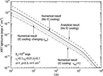
X-ray (0.2–10 keV) afterglow light curves: analytical (dashed line) light curve, and numerical (solid line) when Inverse Compton effect has been ignored. The divergence is about a factor of 2. Numerical estimates when the inverse Compton effect has been taken into account with (dotted line) and without (dashed–dotted line) a Klein–Nishina correction. Clearly, the Klein–Nishina correction is unimportant for the fiducial parameters listed in the figure.

2.2 The GRB efficiency of Swift GRBs with X-ray flattening

Early flattening is evident for a good fraction of the X-ray afterglow light curves recorded by the Swift XRT. Determination of the GRB efficiency of these GRBs is quite challenging since, as we see in Section 4 the underlying physical process that controls the slow decline is unclear. A common interpretation for this flat decay is energy injection, which essentially increases the required initial GRB efficiency. In spite of the uncertainties concerning the applicability of this model we consider its implication to the efficiency.

The energy injection is characterized by a factor f such that fE_k(f∼ a few tens; in the following discussion, we take f= 5) is the energy injected into the fireball (Zhang et al. 2005). The initial GRB efficiency should be

10

where ε_γ≡E_γ/(E_γ+f E_k) is the GRB efficiency derived at t_d∼ 0.4. LZ04 find that ε_γ > 0.4, and therefore, ⁠, which is too high within the framework of the standard (internal shocks) fireball model. However, as shown in Section 2.1, ε_γ presented in LZ04 has been overestimated significantly. We suggest that ε_γ∼ 0.1, therefore even when correcting for the additional energy ⁠, which is still consistent with this model.

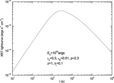
As an example, we consider the γ-ray efficiency of GRB 050319. Both the optical (Mason et al. 2006) and the X-ray (Cusumano et al. 2006) light curves are well recorded for this burst and can be used to constrain the efficiency (see Section 4.1 for a detailed discussion). (1) The time-averaged optical-to-X-ray spectrum (t∼ 200–900 s) is a single power law with an index β=−0.8 (Mason et al. 2006). This implies that ν_m(t∼ 100 s) < ν_R= 4.3 × 10¹⁴ Hz. (2) The very early R-band observation suggests that F_ν,max(t∼ 100 s) ∼ 1 mJy (assuming that energy injection takes place at t≥ 400 s). (3) ν_c > ν_X∼ 10¹⁷ Hz holds up to t∼ 10⁶ s, as suggested by the XRT spectrum. We have (see equations 31–33) ε_e∼ 4 × 10⁻², ε_B∼ 4 × 10⁻⁵, and E_k∼ 1.3 × 10⁵⁴ erg (the energy carried by the initial outflow). With K-correction, the isotropic energy of the γ-ray emission of GRB 050319 is E_γ∼ 1.2 × 10⁵³ erg (Nousek et al. 2005), so ⁠. It is sufficiently low to be well understood within the standard fireball model.

3 MODELS FOR A SLOWLY DECAYING X-RAY AFTERGLOW

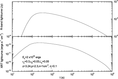
We turn now to explore (both analytically and numerically) models that can give rise to a slowly decaying X-ray afterglow phase. The models we discuss include: (i) energy injection; (ii) a small ζ_e; (iii) evolving shock parameters and (iv) a very low non-constant circumburst density. We also examine the possibility of the X-ray flattening is attributed to a highly magnetized outflow. In the numerical calculations that we present the parameters are chosen to reproduce the XRT light curve of GRB 050319 (for t > 380 s). We also present the corresponding R-band light curve.

3.1 Energy injection

In the standard fireball model, the fireball that is sweeping the circumburst matter decelerates and its bulk Lorentz factor evolves with the time as Γ∝t^−3/8. With continuous significant energy injection, the fireball decelerates more slowly and slowly decaying multiwavelength afterglows are expected. This model has been analytically investigated by many authors (Sari & Mészáros 2000; Nousek et al. 2005; Zhang et al. 2005; Granot & Kumar 2006; Panaitescu et al. 2006). As shown in Zhang et al. (2005), for dE_inj/dt∝t^−q we find ν_m∝t^−(2+q)/2, ν_c∝t^(q−2)/2 and F_ν,max∝t^1−q. In this subsection, we take q= 0.5 and find

11

Following Zhang et al. (2005), we consider an energy injection rate of the form (1 +z) dE_inj/dt=Ac²(t/t₀)^−q for t₀ < t < t_e, where A is a constant. With the energy injection, equation (8) of Huang et al. (2000) should be replaced by (see also Wei, Yan & Fan 2006)

12

where M_ej is the rest mass of the initial GRB ejecta, m is the mass of the medium swept by the GRB ejecta, which is governed by dm= 4πR²n m_p dR, m_p is the rest mass of proton, is the radiation efficiency. Our numerical results, the R-band emission and the 0.2–10 keV emission, are shown in Fig. 2.

Figure 2

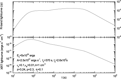
The X-ray (0.2–10 keV) afterglow light curve and the R-band light curve for the energy injection model.

3.2 Small ζ_e

In the standard afterglow model, it is assumed that a fraction ε_e of the shock energy is given to all the fresh electrons that are swept by the shock front. However, it is possible that only a fraction ζ_e of fresh electrons has been accelerated, as suggested by Papathanassiou & Mészáros (1996). With this correction, equations (2) and (3) take the form

13

14

respectively.

For ⁠. A steeper decline is possible (the steepest one is F${}_{\text{ν}{}_{\text{X}}}$∝t^−4/7), depending on the radiative correction, as shown in the upper panel of fig. 2 of Sari et al. (1998).

The transition of the slow decline to a normal decline (F${}_{\text{ν}{}_{\text{X}}}$∝t^−1.2) usually takes place at t∼ 0.1 d or earlier, when ν_X=ν_m. So we have

15

The numerical light curve is presented in Fig. 3. One can see that a long-time multiwavelength flattening is evident with a small ζ_e.

Figure 3

The X-ray (0.2–10 keV) afterglow light curve and the R-band light curve for the small ζ_e model.

Before and after the temporal decline transition, the energy spectrum of the XRT observation should be F_ν∝ν^−1/2 and F_ν∝ν^−p/2, respectively. In other words, after the break in the light curve, the X-ray spectrum should be much softer (see also Zhang et al. 2005), which is inconsistent with most XRT observations (Nousek et al. 2005). In addition, in this model, the spectral index of the XRT afterglows in the slow decline phase is −1/2. It is much harder than that of most Swift X-ray afterglows (see table 1 of Nousek et al. 2005). The Swift observations therefore provide us robust evidences of that significant part of, rather than a small fraction of electrons, have been accelerated in the shock front.

3.3 Evolving shock parameters

In the standard afterglow model, the shock parameters ε_e and ε_B are assumed to be constant. However, it is also possible that ε_e or ε_B, or both, vary with time (see Yost et al. 2003, for detailed discussion). Fan et al. (2002) and Wei, Yan & Fan (2006) modelled the optical flares detected in GRB 990123 and GRB 050904 and found that both ε_e and ε_B of the forward shock (ultrarelativistic) and reverse shock (mild relativistic to relativistic) were very different. This provides an indication evidence for a dependence of the shock parameters on the strength of the shock. Possible evidence for the shock strength-dependent ε_B was also found by Zhang, Kobayashi & Mészáros (2003), Kumar & Panaitescu (2003), McMahon, Kumar & Panaitescu (2004), Panaitescu & Kumar (2004), Fan, Zhang & Wei (2005b) and Blustin et al. (2006). Yost et al. (2003) and Ioka et al. (2005) considered afterglow emission assuming ε_B and ε_e are time-dependent, respectively. Here we simply take (ε_e, ε_B) ∝ (Γ^−a, Γ^−b) for Γ > Γ_o,  otherwise (ε_e, ε_B) ∼ constant, where Γ_o is the Lorentz factor of the outflow at the X-ray decline translation, both a and b are taken to be positive. For simplicity, we discuss only the case of a=b for Γ > Γ_o. Below Γ_o, the solution is the usual one.

The typical synchrotron radiation frequency ν_m satisfies

16

where Γ≈ 25 E^1/8_iso,53[2/(1 +z)]^−3/8t^−3/8_d,−1n^−1/3₀.

The cooling frequency ν_c satisfies

17

The maximum spectral flux F_ν,max satisfies

18

The observed flux behaves as (in this subsection, we take a= 1)

19

The afterglow light curves are shown in Fig. 4. As both ε_e and ε_B increase with time, the flux of the early X-ray emission is dimmer than that of the constant shock parameters model and the decline is much slower. Both are consistent with the current Swift XRT observations (Nousek et al. 2005).

Figure 4

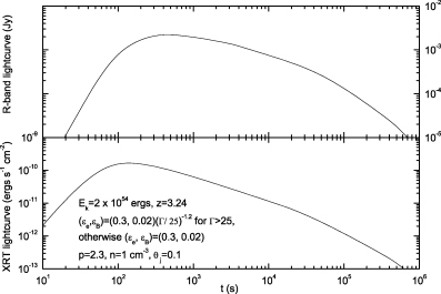
The X-ray (0.2–10 keV) and R-band afterglow light curves for the evolving shock parameter model. The parameters are listed in the figure.

3.4 A very low non-constant density

In the standard interstellar medium (ISM) afterglow model, the number density of the medium is taken as a constant. In the wind model, the number density n decreases with the radius R as n∝R⁻² (Mészáros et al. 1998; Dai & Lu 1998b; Chevalier & Li 2000). Here we discuss the general case n∝R^−k (0 ≤k < 3).

First, we show that for a fireball decelerating in the Blandford–McKee self-similar regime (Blandford & McKee 1976), no X-ray flattening is expected regardless of the choice of k. The energy of the fireball is nearly constant and it is given by E_iso≈Γ²M c², where M∝R^3−k is the total mass of the swept medium. So Γ∝R^−(3−k)/2. Considering that dR∝Γ² dt∝R^−(3−k) dt, we have R∝t^1/(4−k) and Γ∝t^{−(3−k)/[2(4−k)]}.

Now ν_m decreases with t as

20

and ν_c and F_ν,max satisfy

21

22

respectively. This results in

23

The last two are independent of k. So no X-ray flattening appears.

However, if the number density is sufficiently low, the deceleration time-scale (∝n^−1/3) can be very long and even as long as ∼10⁴ s. In this case, a slowly decaying X-ray afterglow may be obtained. One example has been plotted in Fig. 5, in which the density profile of the medium is taken as n= 10⁻⁴ cm⁻³ for R≤ 10¹⁶ cm, n= 10⁻⁴R⁻¹₁₆ cm⁻³ for 1 ≤R₁₆≤ 10³ and n= 10⁻⁷ cm⁻³ for R₁₆ > 10³. An X-ray flattening appears when the shock front reaches R= 10¹⁹ cm. However, while the shape of the light curve is correct the X-ray flux is too low to account for most XRT light curves.

Figure 5

X-ray (0.2–10 keV) afterglow light curve for a very low non-constant density: n= 10⁻⁴ cm⁻³ for R < 10¹⁶ cm; n= 10⁻⁴ (R/10¹⁶)⁻¹ cm⁻³ for 10¹⁶ < R < 10¹⁹ cm and n= 10⁻⁷ cm⁻³ for R > 10¹⁹ cm.

3.5 Magnetized outflow

A Poynting flux dominated outflow (Lyutikov & Blandford 2003; Thompson 1994; Usov 1994) is an alternative to the standard baryonic fireball model. Within the context of this discussion it is of interest since it may also give rise to a slowly decaying X-ray afterglow (Zhang et al. 2005). We investigate, here, briefly this possibility, extended discussion will be presented elsewhere.

We assume that the electromagnetic energy E_p will be transformed continuously into the kinetic energy of the forward shock. The dynamical evolution of the shocked medium is governed by (Huang et al. 2000; Wei et al. 2006)

24

where E_p≡Γ²VB′²/(4π), V is the volume of the magnetized outflow (measured by the observer) and B′ is the comoving strength of the magnetic field.

If the magnetic pressure is higher than the thermal pressure of the shocked medium, the magnetic pressure works on the shocked medium and the kinetic energy of the forward shock increases. A pressure balance between the shocked medium and the magnetized outflow is established, so we have (see also Lyutikov & Blandford 2003) B′²/(8π) =p_gas≃ 4Γ²nm_pc²/3, where p_gas is the thermal pressure of the shocked medium. Therefore, E_p can be estimated by4

25

dE_p/c² can be calculated as follows. Assuming that the whole system (the shocked medium and the magnetized outflow) is adiabatic (i.e. the radiation efficiency ε= 0), the energy conservation yields

26

where V_tot≈ 4πR²Δ is the total volume of the system, Δ is the width of the system, which is described by dΔ= (β_fsh−β) dR and is the velocity of the forward shock. Differentiating equation (26) we obtain

27

After simple algebra, equation (24) can be rearranged as (note that now we take ε= 0)

28

where A= 1 for dE_p/dR≤ 0, otherwise A= 0; B= 32Aπn m_pΓ⁴R[(β_fsh−β)R+ 2Δ].

With proper boundary conditions and the relations dm= 4πn m_pR² dR, dR=βcΓ²(1 +β) dt/(1 +z), V_tot= 4πR²Δ and dΔ= (β_fsh−β) dR, equation (28) can be solved numerically. In our numerical example, we take E_k= 10⁵² erg, n= 1 cm⁻³, E_p= 10E_k and the width of the outflow is taken as 3 × 10¹¹ cm. The starting point of our calculation is at R= 2 × 10¹⁶ cm (∼R_dec, the deceleration radius of the outflow, where ∼E_k/2 has been given to the shocked medium), at which Γ= 360.5 We find out that most of the magnetic energy has been converted into the kinetic energy of the forward shock in a very short time ∼50(1 +z) s. A similar result has been obtained by Lyutikov & Blandford (2003). Though this time-scale is much longer than the crossing time of the reverse shock, it is not long enough to account for the X-ray flattening detected in most GRBs.

4 CASE STUDIES: CONSTRAINING THE MODELS

GRB 050319 and GRB 050401, have well-recorded X-ray and optical afterglows, with which the models discussed in Section 3 can be constrained. We discuss these constraints in detail here. For most Swift GRBs only the X-ray afterglow is well detected. Such bursts provide, of course, much weaker constraints on the model. We discuss one example, GRB 050315, briefly.

4.1 GRB 050319

Both the optical and X-ray afterglows of GRB 050319 have been well recorded (Mason et al. 2006; Nousek et al. 2005; Woźniak et al. 2005; Cusumano et al. 2006). The optical flux declines with a power-law slope of α=−0.57 between ∼200 s after the burst onset until it fades below the sensitivity threshold of the UVOT after 5 × 10⁴ s. The optical V-band emission lies on the extension of the X-ray spectrum, with an spectral slope β=−0.8 (Mason et al. 2006). The temporal behaviour of the X-ray afterglow is more complicated. After a steep decay (α=−5.53) up to t= 370 s, the light curve shows a slow decay with a temporal index of α=−0.54. It steepens to α=−1.14 at t= 2.60 × 10⁴ s. The spectral indices in the slow decline phase and the normal decay phase are β=−0.7 and β=−0.8, respectively (Cusumano et al. 2005; Nousek et al. 2005, However, see Quimby et al. 2006). Below we examine whether the models discussed above (in Section 3) can explain both the optical and the X-ray afterglows self-consistently.

Energy injection: The energy injection model is believed to able to explain the observation (e.g. Cusumano et al. 2005; Mason et al. 2006; Zhang et al. 2005). As shown in Section 3.1, for q= 0.6 and p= 2.4, both the optical and the X-ray afterglows decline as F${}_{\text{ν}{}_{\text{X}}}$∝t^−0.54 when ν_m < ν_R < ν_X < ν_c, the corresponding spectral index should be β=−(p− 1)/2 ∼−0.7. All these values are consistent with the observation. However, the non-detection of the further X-ray break caused by the spectral translation (ν_c < ν_X) up to ∼10⁶ s after the trigger suggests that ε_B∼ 5 × 10⁻³ and n∼ 10⁻³ cm⁻³ (Cusumano et al. 2005). The problem is that F${}_{\text{ν}{}_{\text{X}}}$ depends on n and ε_B sensitively for ν_X < ν_c (see equation 7). The smaller n and ε_B, the smaller F${}_{\text{ν}{}_{\text{X}}}$⁠. We show below that it is quite difficult to reproduce the detected X-ray and optical light curves with the energy injection model.

The earliest R-band data is collected at ∼200 s (note that the real onset of GRB 050319 is about 130 s before the Swift trigger time taken in Woźniak et al. 2005, see Cusumano et al. 2005 for clarification), and the flux is about F${}_{\text{ν}{}_R}$∼ 0.7 mJy. At that time, the total energy of the outflow is still dominated by the initial E_k, and F_ν,max and ν_m are still described by equations (2) and (3), respectively. The conditions F_ν,max≥ 0.7 mJy and ν_m(t∼ 200 s) ≤ν_R yield

29

30

respectively. The condition ν_c≥ν_X∼ 10¹⁷ Hz holding up to t∼ 10⁶ s gives

31

where Y_o is the Compton parameter at t∼ 10⁶ s. To derived this relation, we assume that at t∼ 200 s, ν_c is described by equation (4), and ν_c∝t^(q−2)/2∼t^−0.7 up to t∼ 2.6 × 10⁴ s (i.e. in the energy injection phase), then ν_c∝t^−1/2 up to t∼ 10⁶ s.Combing equations (29–31), we have

32

33

Now Y₀∼ 0 (see Appendices A and B for detail), we have E_k > 1.3 × 10⁵⁴ erg n^−1/5₀. On the other hand, the energy injection coefficient A′≡Ac²∼ (1 +z)E_k/t₀∼ 1.4 × 10⁵²n^−1/5₀ erg s⁻¹ for t₀∼ 370 s. Please note that A′ is comparable to the recorded luminosity of most GRBs and the X-ray luminosity recorded by XRT is just ∼10⁴⁸ erg s⁻¹. The outflow accounting for the late-time injection is so energetic that strong soft X-ray to γ-ray emission powering by shocks or magnetic dissipation are expected. They will quite likely dominate over the corresponding forward shock emission, which is inconsistent with the observation.

This model is also disfavoured by the different temporal behaviour of the X-ray and the optical afterglows at t > 2.6 × 10⁴ s. We therefore conclude that the energy injection model cannot account for the multiwavelength afterglows of GRB 050319. We tried to fit both the R-band and X-ray afterglows with reasonable parameters numerically but failed.

Provided that the energy injection model works (i.e. there is a mechanism to keep such energetic outflow steady enough and there is no magnetic dissipation), the initial GRB efficiency in this case is as low as ⁠.

Smallζ_e: This model is disfavoured by two facts. One is that in the X-ray flattening phase, ν_c < ν_X < ν_m, the corresponding spectral index is β∼− 1/2, which only marginally matches the observation ∼−0.7. The other is that after the temporal transition at t∼ 10⁴ s, ν_c < ν_m < ν_X, the spectral index should be β=−p/2 ∼−1.2, which is inconsistent with the observation.

Evolving shock parameters: As shown in Section 3.3, for ν_m < ν_R < ν_X < ν_c, p= 2.4 and a=b= 0.6, (F${}_{\text{ν}{}_R}$⁠, F${}_{\text{ν}{}_{\text{X}}}$⁠) ∝t^−0.54 and the spectral index β=−(p− 1)/2 ∼−0.7, are all consistent with the observation. After the shock parameters saturate at t∼ 2.6 × 10⁴ s, F${}_{\text{ν}{}_{\text{X}}}$∝t^−1.1 and β=−0.7 as long as ν_X < ν_c, which also matches the observation. However, the optical light curve should be much steeper since ν_m < ν_R < ν_c also holds. The UVOT observation and the ground basedR-band observation suggest that the decline of optical emission does not change up to t∼ 2 × 10⁵ s, though the scatter of the flux is quite large (Kiziloglu et al. 2005; Sharapov et al. 2005; see Mason et al. 2006 for a summary). Therefore the evolving shock parameter model is disfavoured.

Very low non-constant density: With proper parameters as well as proper density profile, an X-ray flattening does appear (see Fig. 5). However, as already mentioned, the flux is too low to match most observations, here we do not discuss it further.

Off-beam annular jet model: Recently, Eichler & Granot (2006) suggested that the flat part of the XRT light curve may be a combination of the decaying tail of the prompt γ-ray emission and the delayed onset of the afterglow emission observed from viewing angles slightly outside of the edge of the jet (i.e. off-beam). This model, like others mentioned above, can account for the slow decline of many X-ray afterglows, but may be unable to explain both the optical and the X-ray afterglows of GRB 050319 self-consistently, as shown below.

Following Eichler & Granot (2006), we assume that the off-beam angle is δθ∼ 1/Γ_int, where Γ_int is the initial Lorentz factor of the outflow. Larger δθ is less favoured since the slowly decaying R-band afterglow has been well recorded as early as t∼ 200 s, which implies that the afterglow onset has not been delayed so much. In the off-beam case, the typical synchrotron radiation frequency should be

34

where a≈[1 + (Γ_intδθ)²]∼ 2 is the Doppler factor. Therefore, the condition ν_m(t∼ 200 s) < ν_R results in

35

For δθ∼ 1/Γ_int, the late-time (i.e. the normal decline phase) afterglow emission is quite similar to the on-beam case (Eichler & Granot 2006).

We use equation (7) to estimate the late-time X-ray flux, though the predicted flux of the annular jet model should be somewhat different from that of our conical jet model (Eichler & Granot 2006; Granot 2005). The XRT flux ≈8 × 10⁻¹² erg s⁻¹ cm⁻² at t_d∼ 0.3 gives

36

The condition ν_c > ν_X∼ 10¹⁷ Hz holding up to t∼ 10⁶ s yields

37

Combing equations (35–37), we have E_k > 10⁵⁵ erg n^−1/5₀ (a/2)^3(p−1)/10. While we manage to fit both X-ray and optical data, the energy needed is too large for any realistic progenitor models. We therefore suggest that the off-beam annular jet model is also unable to account for the afterglows of GRB 050319.

4.2 GRB 050401

The early X-ray light curve is consistent with a broken power law with α=−0.63 and −1.41 respectively, the break is at t_b∼ 4480 s (de Pasquale et al. 2006). The X-ray spectral indices before and after the break are nearly constant ∼−0.90. Therefore, the small ζ_e model is ruled out directly. Zhang et al. (2005) also show that the flat electron distribution model (1 < p < 2) is unable to account for the X-ray afterglow observation. The afterglow has also been detected in R-band, which decays as a simple power law ∝t^−0.76 up to t∼ 3.5 × 10⁴ s (Rykoff et al. 2005).

Energy injection(p∼ 2.8): After the break, the light curve is consistent with an ISM model for ν_m < ν_X < ν_c with p∼ 2.8. Before the break, it is consistent with the same model with q= 0.5 (see also Zhang et al. 2005). As far as the R-band afterglow emission is concerned, there are two possibilities. One is that ν_m < ν_R < ν_c, the optical afterglow should follow the temporal behaviour of the X-ray afterglow, which is not the case. The other is that ν_R < ν_m for t≤t_b, the afterglow increases as t^0.9 for q∼ 0.5 (see Section 3.1), which is inconsistent with the observation. We therefore conclude that the popular energy injection model is unable to account for the data in this burst as well.

Evolving shock parameters(p∼ 2.8): The light curve after the break is consistent with an ISM model for ν_m < ν_X < ν_c with p∼ 2.8. Before the break, it is consistent with the same model with a=b= 0.7. Can it reproduce the optical afterglow? The answer is negative. Provided that ν_R < ν_m for t≤t_b, the optical afterglow should increase as t^0.4 (see Section 3.3), which is inconsistent with the data. The case of ν_m < ν_R is ruled out directly in view of the different temporal behaviour of X-ray and R-band afterglows.

4.3 GRB 050315

After a steep decay up to t_b1= 308 s, the X-ray light curve shows a flat ‘plateau’ with a temporal index of α=−0.06 (the spectral index of XRT data is β=−0.73). It then turns to α=−0.71 at t_b2= 1.2 × 10⁴ s, the spectral index is β=−0.79. Finally, there is a third break at t_b3= 2.5 × 10⁵ s, after which the temporal decay index is α=−2.0 and the spectral index is β=−0.7 (Barthelmy et al. 2005; Nousek et al. 2005).

There are two possible interpretations for the long-term constant spectral index β∼−0.7. One is that max{ν_c, ν_m} < ν_X after t= 308 s and the power-law index of the shocked electron p∼ 1.5. The other is that ν_m < ν_X < ν_c for t_b1 < t < t_b3 and p∼ 2.5.

Energy injection(p∼ 2.5): To obtain the slow decline for t_b1 < t < t_b2, energy injection with q∼ 0.2 is needed. q∼ 0.9 is needed to reproduce the X-ray afterglows at t_b2 < t < t_b3. The late-time sharp decay appears when the boundary of a non-spreading jet becomes visible.

Evolving shock parameters(p∼ 2.5): As shown in Section 3.3, with a=b= 1.2, we have a slow decline slope α=−0.06 between t_b1 and t_b2. To get a decline slope α=−0.71 between t_b2 and t_b3, a=b= 0.45 are needed. The late-time sharp decay appears when the boundary of a non-spreading jet becomes visible and a=b= 0.45.

We find that both models can explain the observed X-ray light curves of GRB 050315.

5 SUMMARY AND DISCUSSION

During the past several months, the Swift XRT has collected a rich sample of early X-ray afterglow data. A good fraction of these afterglows show a slow decline phase lasting between a few hundred to several thousand seconds. The energy injection model is the leading model to account for these slowly decaying X-ray afterglows (e.g. Nousek et al. 2005; Zhang et al. 2005; Granot & Kumar 2006; Panaitescu et al. 2006). It has been suggested that in this model, the GRB efficiency might be as high as 90 per cent. Such a high-efficiency challenges the standard internal shock model for the prompt γ-ray emission.

In this work, we have re-examined the GRB efficiency of several pre-Swift GRBs and one Swift GRB. In addition, we have explored several mechanism which might give rise to a slowly decaying X-ray light curve and we have compared the predictions of these models with the well-recorded multiwavelength afterglows of GRB 050319 and GRB 050401. We draw the following conclusions:

1. The GRB efficiency of pre-Swift GRBs that has been derived directly from the X-ray flux 10 h after the burst has been overestimated. For these Swift GRBs with long-time X-ray flattening, the GRB efficiency is also moderate (around 0.5), even when taking into account the possibility of energy injection. Such efficiency can be understood within the standard internal shock model.

2. With a proper choice of parameters, the slow decline slope of X-ray afterglow like the one detected in GRB 050319 can be well reproduced by several models – the energy injection model, evolving shock parameter model (in which the shock parameters are assumed to increase with the decrease of the shock strength for t < 10⁴ s), the small ζ_e model (in which the shock energy has been give to a fraction ζ_e of electrons, rather than total) and the very low non-constant density model. Out of these models, the last two are ruled out by the X-ray data itself. In the last model, the resulting X-ray afterglow is too dim to match most XRT observations. The small ζ_e model is also disfavoured since (1) in the slow decline phase, the XRT spectrum are usually much softer than ν^−1/2; (2) after the light-curve break, no spectral steepening has been detected in most cases, which is inconsistent with the model. The other models, including the energy injection model and the evolving shock parameter model seem to be consistent with the X-ray afterglow observations.

3. While two models, the energy injection model and the evolving shock parameter model, are consistent with the X-ray data, they fail to reproduce both the X-ray and the optical afterglows of GRB 050319 and GRB 050401. In each burst, the optical flux declines slowly up to ∼10⁵ s. On the other hand, the X-ray light curve decays slowly up to t∼ 10⁴ and then turns to the normal faster decay (F∝t^−1.2 or so). The temporal index of the slow decay X-ray phase is close to that of the optical light curve. The XRT spectrum is unchanged before and after the X-ray break. This means that the break is not caused by a cooling break in which ν_c crosses the observed frequency.

The failure of all models that we considered to fit both the X-ray and the optical afterglow light curves suggests that we should look for another alternative. An intriguing possibility is based on fact that the extrapolation backwards of the late X-ray light curve is in agreement with (or 1–2 order lower than) the prompt X-ray emission. This suggests that we face a ‘missing energy problem’. Namely, during the slow decay phase (in which the X-ray flux is rather low) we miss X-ray emission. Is it possible that during this phase this energy is dissipated into a different channel and not into synchrotron X-rays and that this different channel becomes ineffective at around 10 h? Put differently, during this phase the electrons within the forward shock emit synchrotron X-rays inefficiently. A possibility of this kind (that we have considered and found not to work) is if the X-ray emitting electrons are cooled efficiently via inverse Compton (and hence their synchrotron X-ray emission is weaker). As already mentioned inverse Compton cooling is important in determining the X-ray flux. Furthermore, due to the Klein–Nishina cut-off this cooling becomes unimportant at approximately 1 d. However, this transition is not sharp enough to produce the observed slowly decaying X-ray light curves. While inverse Compton cooling does not work it is possible that another, yet unexplored, process of this kind is responsible for the observed light curves.

We thank A. Panaitescu and E. Waxman for their constructive comments. We also thank the referee for helpful suggestion. YF thanks D. M. Wei for his help and J. Dyks for checking Fig. 5. This work is supported by US-Israel BSF. TP acknowledges the support of Schwartzmann University Chair. YF is also supported by the National Natural Science Foundation (grants 10225314 and 10233010) of China, and the National 973 Project on Fundamental Researches of China (NKBRSF G19990754).

1

If the outflow ejected from the central engine after the GRB phase is highly magnetized, at a radius ∼10¹⁵ cm, the magnetohydrodynamics (MHD) condition breaks down. Significant magnetic field dissipation processes are expected to happen which converts energy into radiation. As long as the highly magnetized outflow is steady enough, strong and slowly decaying X-ray emission is possible (see Fan, Zhang & Proga 2005a and the references therein).

2

To derive these equations, the deceleration of the fireball is governed by the energy conservation Γ²M c²=E_k, where M is the rest mass of the shocked medium (e.g. Blandford & McKee 1976; Sari et al. 1998; Piran 1999). The distribution of the fresh electrons accelerated by the shock is assumed to be dn/dγ_e∝γ^−p_e for γ_e≥γ_e,m, where γ_e,m= (m_p/m_e)[(p− 2)/(p− 1)]ε_e(Γ− 1), governed by the strict shock jump conditions (Blandford & McKee 1976). The other crucial parameter is the cooling Lorentz factor γ_e,c= 6(1 +z) πm_ec/[σ_TΓB²t(1 +Y)], above which the energy loss due to the synchrotron/inverse Compton radiation is important (Sari et al. 1998; Piran 1999), where σ_T is the Thompson cross-section and B is the magnetic field of the shocked medium. ν_m and ν_c are the corresponding synchrotron radiation frequency of electrons with Lorentz factors γ_e,m and γ_e,c, respectively. The maximum specific flux is estimated as F_ν,max≈ (1 +z)MΓe³B/(4πm_pm_ec²D²_L) (Sari et al. 1998; Wijers & Galama 1999), where e is the charge of electron. The ν_c and F_ν,max taken here are comparable with that of most previous works (e.g. Granot, Piran & Sari 1999; Wijers & Galama 1999; Panaitescu & Kumar 2002; LZ04). The ν_m is close to that taken in Sari et al. (1998), Granot et al. (1999) and Wijers & Galama (1999), but is about 30–40 times smaller than that taken in Panaitescu & Kumar (2002) and LZ04. Such a large divergency may arise if one ignores the term (p− 2)/(p− 1) when evaluating γ_e,m.

3

While our results are very close to the recent calculations of Granot et al. (2006), they also show that the estimates of E_k are very sensitive to the exact expressions used for ν_c, ν_m and F_ν,max. Similar conclusion can be drawn by comparing previous results of Granot et al. (1999), Wijers & Galama (1999), Freedman & Waxman (2001), Panaitescu & Kumar (2002) and LZ04. Therefore, an alternative explanation for the apparent high efficiencies is that the blast wave energy estimates using L_X are simply inaccurate.

4

Providing that V∝R^2+cΓ^−d, E_p∝Γ^8+2c-dt^2+c∝t^−δ (c, d and δ are all larger than 0), we have Γ∝t^{−(2+c+δ)/(8+2c−d)}, which should be flatter than Γ^−3/8 (the canonical dynamical evolution of a ejecta without energy injection). It requires that 2c+ 3d < 8 − 8δ, otherwise dE_p/dt < 0 has been violated. It is evident that in the spreading phase, i.e. c= 1 and d= 2, E_p can not be converted into the kinetic energy of the forward shock effectively.

5

At that radius, the reverse shock has crossed the ejecta and a pressure balance between the shocked medium and the magnetized outflow is reached. In this work, we do not calculate the reverse shock emission (see Fan, Wei & Wang 2004a) for the reverse shock emission with mild magnetization and Zhang & Kobayashi (2005) for reverse shock emission with arbitrary magnetization. With the ideal MHD jump condition, the reverse shock can not convert the magnetic energy into the kinetic energy of the forward shock effectively, as shown in Kennel & Coronitti (1984), Fan, Wei & Zhang (2004b) and Zhang & Kobayashi (2005) both analytically and numerically.

APPENDIX A: THE GENERAL FORM OF THE INVERSE COMPTON PARAMETER

For the photons with frequency higher than ⁠, the Compton parameter should be suppressed significantly since it is the Klein–Nishina regime, where is governed by ⁠, i.e.

(A1)

We extend the derivation of the Compton parameter Y given by Sari et al. (1996) to the general form, in the limit of single scattering. The ratio of the inverse Compton power (P_IC) to the synchrotron power (P_syn) of an electron with random Lorentz factor γ_e is given by

(A2)

where η_KN is the fraction of synchrotron radiation energy of total electrons emitted at frequencies below ⁠. So we have

(A3)

Below we estimate the parameter η_KN in different cooling regimes.

A1 Slow cooling

(A4)

where ν_M∼ 2.8 × 10²²Γ/(1 +z) Hz is the maximal synchrotron radiation frequency of the electrons accelerated by the forward shock. For p > 2, the total energy emitted is ⁠, where the photons with frequencies below ν_m have been ignored. Throughout the appendix, ν_c is still described by equation (4) but without the correction of 1/(1 +Y)². We have

(A5)

For 1 < p < 2, the total energy emitted is ⁠, where S₁=[(3 −p)ν^1/2_cν^(2−p)/2_M−ν^(3−p)/2_c− (2 −p) ν^(3−p)/2_m]. Now η_KN can be estimated as

(A6)

A2 Fast cooling

(A7)

For p > 2, the total energy emitted is ⁠, where the emission below ν_c has been ignored. The η_KN is estimated as

(A8)

For 1 < p < 2, the total energy emitted is ⁠, where S₂=[ν^(p−1)/2_mν^(2−p)/2_M− (p− 1) ν^1/2_m− (2 −p)ν^1/2_c]. We have

(A9)

APPENDIX B: WHEN IS THE KLEIN–NISHINA CORRECTION IMPORTANT?

In the shock front, the magnetic field strength B is

(B1)

The typical synchrotron radiation frequency of an electron with random Lorentz factor γ_e is

(B2)

B1 The XRT light curve

For ν_X∼ 10¹⁷ Hz, we have γ_e(ν_X) = 1.3 × 10⁵[2/(1 +z)]^−1/2Γ⁻¹₁ε^−1/4_B,−2n^−1/4₀ and

(B3)

Therefore, the Klein–Nishina correction seems to be unimportant (i.e. η_KN∼ 1) for t_d∼ 1 (when ⁠) and ε_B∼ 0.01.

B2 The R-band light curve

For ν_R∼ 4.3 × 10¹⁴ Hz, we have γ_e(ν_R) = 8 × 10³[2/(1 +z)]^−1/2Γ⁻¹₁ε^−1/4_B,−2n^−1/4₀ and

(B4)

Then, with ε_B∼ 0.01, the Klein–Nishina correction seems to be unimportant for a long time. On the other hand, the factor η≃ min {1, (ν_m/ν_c)^(p−1)/2}∼ 1 for t_d < 1. As a consequence, the inverse Compton effect is very important both for the long wavelength afterglow calculation and for the X-ray light-curve calculation. However, it may be unimportant for a lower ε_B since ν_c∝ε^−3/2_B.

Author notes

†

Lady Davis Fellow.