Precise photometric redshifts with a narrow-band filter set: the PAU survey at the William Herschel Telescope

Abstract

The Physics of the Accelerating Universe (PAU) survey at the William Herschel Telescope will use a new optical camera (PAUCam) with a large set of narrow-band filters to perform a photometric galaxy survey with a quasi-spectroscopic redshift precision of σ(z)/(1 + z) ∼ 0.0035 and map the large-scale structure of the universe in three dimensions up to i_AB < 22.5–23.0. In this paper, we present a detailed photo-z performance study using photometric simulations for 40 equally spaced 12.5-nm-wide (full width at half-maximum) filters with an ∼25 per cent overlap and spanning the wavelength range from 450 to 850 nm, together with a ugrizY broad-band filter system. We then present the migration matrix r_ij, containing the probability that a galaxy in a true redshift bin j is measured in a photo-z bin i, and study its effect on the determination of galaxy auto- and cross-correlations. Finally, we also study the impact on the photo-z performance of small variations of the filter set in terms of width, wavelength coverage, etc., and find a broad region where slightly modified filter sets provide similar results, with the original set being close to optimal.

surveys, galaxies: distances and redshifts, galaxies: statistics, large-scale structure of Universe

1 INTRODUCTION

Galaxy surveys are a fundamental tool in order to understand the large-scale structure (LSS) of the universe as well as its geometry, content, history, evolution and destiny. Spectroscopic surveys (2dF, Colless et al. 2001; VVDS, Le Fèvre et al. 2005; WiggleZ, Drinkwater et al. 2010; BOSS, Dawson et al. 2013) provide a 3D image of the galaxy distribution in the near universe, but most of them suffer from limited depth, incompleteness and selection effects. Imaging surveys (SDSS, York et al. 2000; PanSTARRS, Kaiser, Tonry & Luppino 2000; LSST, Tyson et al. 2003) solve these problems but, on the other hand, do not provide a true 3D picture of the universe, due to their limited resolution in the position along the line of sight, which is obtained measuring the galaxy redshift through photometric techniques using a set of broad-band (BB) filters. The Physics of the Accelerating Universe (PAU) survey at the William Herschel Telescope (WHT) in the Roque de los Muchachos Observatory (ORM) in the Canary island of La Palma (Spain) will use narrow-band (NB) filters to try to achieve a quasi-spectroscopic precision in the redshift determination that will allow it to map the LSS of the universe in 3D using photometric techniques, and, hence, overcoming the limitations of spectroscopic surveys (Benítez et al. 2009).

In this paper, we present the study of the photo-z performance and its impact on clustering measurements expected in the PAU survey in a sample consisting of all galaxies of all types with i_AB < 22.5. Based on detailed simulation studies (Gaztañaga et al. 2012), the requirement for the precision is set at σ(z)/(1 + z) = 0.0035. The PAU survey will observe many galaxies beyond the i_AB = 22.5 limit that play a crucial role in the PAU science case (Gaztañaga et al. 2012). We will also study the performance in a fainter galaxy sample with 22.5 < i_AB ≲ 23.7, expecting to reach a photo-z precision not worse than σ(z)/(1 + z) = 0.05 (Gaztañaga et al. 2012). Finally, we will also study the impact on the photo-z performance of small variations on the default filter set, in terms of width, wavelength coverage, etc.

There are two main sets of techniques for measuring photometric redshifts (or photo-z): template methods (e.g. hyperz, Bolzonella, Miralles & Pell 2000; bpz, Benitez 2000; Coe et al. 2006; lephare, Ilbert et al. 2006; eazy, Brammer, van Dokkum & Coppi 2008), in which the measured BB galaxy spectral energy distribution (SED) is compared to a set of redshifted templates until a best match is found, thereby determining both the galaxy type and its redshift; training methods (e.g. annz, Collister & Lahav 2004; arborz, Gerdes et al. 2010; tpz, Carrasco Kind & Brunner 2013), in which a set of galaxies for which the redshift is already known is used to train a machine-learning algorithm (an artificial neural network, for example), which is then applied over the galaxy set of interest. Each technique has its own advantages and disadvantages, whose discussion lies beyond the scope of this paper.

Throughout the paper, we will be using the Bayesian Photo-Z (bpz) template-based code from Benitez (2000), after adapting it to our needs. We have also tried several photo-z codes based on training methods. We have found that, because of the large, |${\cal O}(50)$|⁠, number of filters, some of them run into difficulties due to the combinatorial growth of the complexity of the problem, while others confirm the results presented here. The results obtained with training methods will be described in detail elsewhere (Bonnett et al., in preparation).

The outline of the paper is as follows. In Section 2, we present the default PAU filter set. Section 3 discusses the mock galaxy samples that we use in our study, the noise generation, and the split into a bright and a faint galaxy samples. In Section 4, we introduce the bpz original code and our modifications, with special emphasis on the prior redshift probability distributions and the odds parameter. We also show the results obtained when running bpz on the mock catalogue using the default filter set. Furthermore, we compute the so-called migration matrix r_ij (Gaztañaga et al. 2012), corresponding to the probability that a galaxy at a true redshift bin j is actually measured at a photo-z bin i, and its effect on the measurement of galaxy auto- and cross-correlations. In Section 5, we try several modifications to the filter set (wider/narrower filters, bluer/redder filters, etc.), study their performance on the brighter and fainter galaxy samples and find the optimal set. Finally, in Section 6, we discuss the results and offer some conclusions.

2 DEFAULT FILTER SET-UP

In this section, we construct the effective filter response R(λ) of the PAU bands and compute their 5σ limiting magnitudes, m_AB(5σ).

2.1 Nominal response

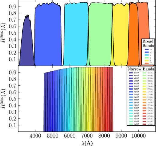
PAUCam will mount two sets of filters: the BB filters, composed of six bands ugrizY,¹ whose nominal (or theoretical) response R^theo(λ) is shown on the top of Fig. 1, and the NB filters, shown on the bottom, which are composed of 40 top-hat adjacent bands with a rectangular width of 100 Å ranging from 4500 to 8500 Å. Since there is a technical limitation to construct such narrow top-hat bands, we relax the transition from zero to the maximum response by adding two lateral wings of 25 Å width, resulting in a full width at half-maximum (FWHM) of 125 Å. This induces an overlap of ∼25 per cent between contiguous bands. Additionally, we set the overall NB response to match that from the ALHAMBRA survey instrument (Moles et al. 2008), which are comparable in technical specifications (although with a wider wavelength range, ∼310 Å, transmission) and have similar coatings.

Figure 1.

The nominal (or theoretical) response R^theo(λ) of the ugrizY PAU BBs (top) and the 40 NBs (bottom). The u band is the same as in the USNO 40-in telescope at Flagstaff Station (Arizona), while the grizY are the same as in the DECam mounted in the Blanco Telescope (CTIO, Chile). The NB filters have a 125 Å FWHM and overlap by 25 per cent with the adjacent bands. They are labelled on the plot through their central wavelength. Their overall response is set to match that of the ALHAMBRA survey bands.

2.2 Effective response

The filter responses R^theo(λ) in Fig. 1 are the nominal: this is the response that we would measure if light went only through the filter. Light also goes through the Earth's atmosphere, which absorbs part of the light, and then, also goes through the optics (mirror and corrector) of the telescope before getting into the filter. Moreover, the CCD detectors behind filters also are affected by a quantum-efficiency (QE) response curve. Therefore, if we want to know the effective response of the filters, we will have to take into account all the transmission curves T_i(λ) of these effects i. In our case, these curves are shown in the top plot of Fig. 2. The QE curve (blue) corresponds to the measured QE of CCDs provided by Hammamatsu, the measured transmission curve of the telescope's optics (mirror + corrector) (green) corresponds to that from the WHT optics and the atmospheric transmission curve (red) is taken from the Apache Point Observatory (APO) at New Mexico. We assume that the APO atmosphere transmission is close enough to the ORM for the purpose of this study. The resulting effective response R(λ) is derived with the expression

\begin{eqnarray} R(\lambda ) &=& R^{\rm theo}(\lambda ) \prod _{i} T_i(\lambda ) \nonumber \\ &=& R^{\rm theo}(\lambda ) T_{\rm CCD}(\lambda ) T_{\rm opt}(\lambda ) T_{\rm atm}(\lambda ). \end{eqnarray}

(1)

The transmission of the WHT optics is less than 50 per cent in all the wavelength range, so that the resulting effective responses are significantly reduced. On the other hand, the three transmission curves T_i(λ) begin to fall when they enter the ultraviolet region (∼3800 Å). Similarly, the CCDs QE drops as we approach the infrared region above ∼9000 Å. Overall, the u and Y BBs are less efficient than the rest. This does not affect the NB, since their wavelength range are within these limits. Atmospheric telluric absorption bands, located between ∼700 nm and ∼1 μm, are also imprinted in the final response of the filters. This is particularly relevant for the NB since their typical width is similar to the width of these valleys. In particular, the profile of the NB with central wavelength at ∼7550 Å (orange) is drastically changed by the telluric absorption A band.

Figure 2.

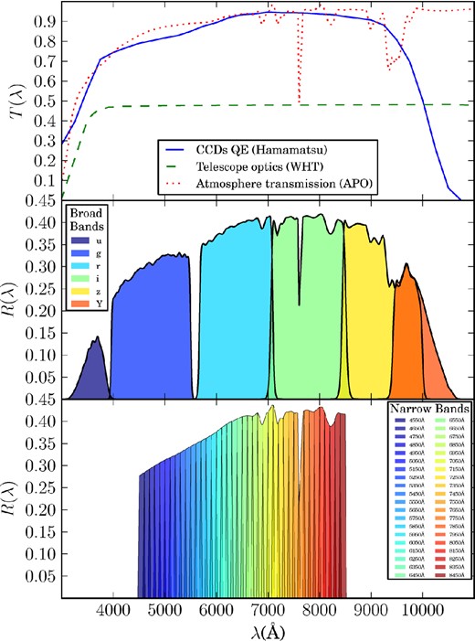
Top: the QE curve (blue) of the PAUCam CCDs, the transmission curve of the WHT optics (green) and the atmospheric transmission (red) at the APO, that affect the final response of the PAU bands. The two lower plots are the same as in Fig. 1, but after taking into account these additional transmission curves T_i(λ) through equation (1). For the sake of clarity, we have rescaled the y-axes due to the low efficiency of the mirror's reflexion.

2.3 5σ limiting magnitudes

Next, we compute the 5σ limiting magnitudes, m_AB(5σ), for all the PAU bands in the AB photometric system² (Oke & Schild 1970). This is the apparent magnitude whose signal-to-noise (S/N) ratio, given by

\begin{equation} {S \over N} = \sqrt{A \over \alpha ^2}{N_{\rm gal} \over \sqrt{N_{\rm gal} + N_{\rm sky} + n {\rm RN}^2} }, \end{equation}

(2)

is equal to 5, where

\begin{eqnarray} N_{\rm gal}&=&3631 \times \ 1.51\times 10^7 \times 10^{-0.4m_{{\rm AB}}} \left({\alpha ^2\over A}\right) \nonumber \\ &&\times \, \pi \left({\phi \over 2}\right)^2 nt_R \int ^{\infty }_0 R(\lambda ) {\rm{d}\lambda \over \lambda }, \end{eqnarray}

(3)

\begin{eqnarray} N_{\rm sky} &=& \alpha ^2 \pi \left({\phi \over 2}\right)^2 nt_R \int ^{\infty }_0 f_{\rm sky}(\lambda ) R(\lambda )\, {\rm d}\lambda , \end{eqnarray}

(4)

are the photons per pixel coming from the galaxy and the sky brightness, respectively, {ϕ, α, RN, A, n} are the parameters of both the WHT and PAUCam instrument, whose values and description are given in Table 1, f_sky(λ) is the spectral density flux per unit of aperture of the sky brightness, whose curve is on top of Fig. 3 and t_R is the exposure time for the filter R(λ). All the filters intended for the photometry are arranged over the central part of the focal plane (FP) where vignetting is practically negligible. NB are distributed through five interchangeable trays. From the bluest to the reddest, each tray carries a group of eight consecutive NB. This gives 5 trays × 8 NB = 40 NB. Values for the exposure times T_i of each tray are shown on the left-hand column of Table 2. On the other hand, each BB filter is mounted into a dedicated tray with its particular exposure time, in such a way that NB and BB exposure times are completely decoupled. Values for the exposure times t_R of each BB filter are shown on the right-hand column of Table 2. The exposure times t_R and the derived limiting magnitudes m_AB(5σ) for each filter are also shown on the middle and bottom plots of Fig. 3, respectively, in a colour degradation for NB and in black for BB. Since f_sky(λ) increases with wavelength, exposure times t_R for redder filters are also set to increase in order to compensate the noise introduced by the sky (note that the exposure times for the NB increase in steps, due to their arrangement in groups per tray). However, this increment is not enough to compensate the sky brightness as we can see with the descending m_AB(5σ) with wavelength. Note that the u band has a lower limiting magnitude compared with g even being at shorter wavelengths. This is because the u response is strongly affected by the transmission curves T_i. Furthermore, there are large drops in m_AB(5σ) for the NB with central wavelength 5550, 6250 and 6350 Å. This is due to emission lines in the sky spectrum f_sky(λ) at these wavelengths.

Figure 3.

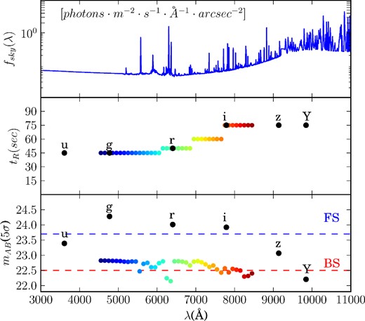
Top: a model of the spectral density flux of the sky brightness f_sky(λ) at La Palma (day 7 on the lunar cycle) assuming an airmass of 1.0, used in equation (4). Middle: the exposure times t_R for each PAU band used in equations (3) and (4). Bottom: the resulting limiting magnitudes m_AB(5σ) for each band computed through equations (2)–(4). Coloured points correspond to NBs and black to BBs.

Table 1.

Description and values of the WHT and PAUCam parameters used in equations (2)–(4), to compute the S/N.

ϕ	Telescope mirror diameter	4.2 m
α	FP scale	0.265 arcsec pix−1
RN	Read-out noise	5 electrons pix−1
A	Galaxy aperture	2 arcsec2
n	# of exposures	2

Table 2.

Left: exposure times T_i for each PAUCam NB filter tray. The individual NB exposure times are equal to those of the tray where they are. Right: the BB exposure times. Exposure times t_R per filter are also shown in the middle plot of Fig. 3.

NB tray Ti		BB tR
T1	45 s	u	45 s
T2	45 s	g	45 s
T3	50 s	r	50 s
T4	60 s	i	75 s
T5	75 s	z	75 s
		Y	75 s

3 THE MOCK CATALOGUE

In this section, we generate a photometric mock catalogue |$\lbrace m_j \pm \sigma _{m_j}, z,t \rbrace$| with observed magnitudes |$m_j\pm \sigma _{m_j}$| in each PAU band j for galaxies at redshift z and with spectral type t.

3.1 Noiseless magnitudes

We use a method similar to the one described in Jouvel et al. (2009), which consists in sampling the cumulative luminosity function (LF)

\begin{eqnarray} N(z,t) = \int _{-\infty }^{M_{\rm lim}(z,t)} \phi x^\alpha {\rm e}^{-x} \rm{d}x \nonumber \\ x\equiv 10^{-0.4(M-M^*)}, \end{eqnarray}

(5)

in the redshift range z = [0, 6], for a total of N ∼ 10⁶ galaxies. M is the absolute magnitude and M_lim(z, t) the absolute magnitude limit at redshift z and spectral type t for a given apparent magnitude limit of the catalogue m_lim in some reference band. In our case, m_lim < 26.0 in the r_SDSS band. Finally, {M*, ϕ, α} are the parameters of the LF, which also depend on z and t. We assume that their redshift dependence is

\begin{equation} \lbrace M^*, \log _{10}\phi , \alpha \rbrace = \lbrace a \exp [-(1+z)^{b}] + c \rbrace , \end{equation}

(6)

where {a, b, c} are type-dependent parameters whose values are in Table 3. These values are chosen to match the LFs and their evolution from Dahlen et al. (2005), where three different spectral types, 1 = Elliptical (Ell), 2 = Spiral (Sp), 3 = Irregular (Irr), are distinguished.

Table 3.

Parameters {a, b, c} that, through equation (6), give the values and evolution in redshift of the LF parameters {log₁₀ϕ, M*, α} for a given spectral type t. These values are based on the LFs in Dahlen et al. (2005), where three galaxy types are distinguished: 1 = Ell, 2 = Sp and 3 = Irr.

	log10ϕ			M*			α
t	a	b	c	a	b	c	a	b	c
1	2.4	1.1	−2.7	5.0	1.6	−21.90	1.7	1.6	−1.00
2	0.5	0.1	−2.28	3.2	2.5	−21.00	0.7	−0.9	−1.50
3	1.0	−3.5	−3.1	5.0	1.3	−20.00	1.8	0.9	−1.85

The relation between the absolute magnitude M and the apparent magnitude m for a galaxy at redshift z and with spectral type t, used in the magnitude limit of equation (5), is

\begin{equation} M = m - 5 \log _{10}D_{\rm L}(z) - 25 - K(z,t), \end{equation}

(7)

where D_L(z) is the luminosity distance of the galaxy at redshift z in Mpc, which in a Λcold dark matter universe is expressed as

\begin{equation} D_{\rm L}(z) \equiv (1+z) {c \over H_0}\int _0^{z} {{\rm d}z \over \sqrt{\Omega _{\rm M}(1+z)^3 + \Omega _\Lambda } }, \end{equation}

(8)

with cosmological parameters chosen to be: H₀ = 75 (km s⁻¹) Mpc⁻¹, Ω_M = 0.25 and |$\Omega _\Lambda$| = 0.75, and K(z, t) is the K-correction

\begin{equation} K(z,t) \equiv -2.5 \log _{10} \left[{1 \over 1+z}{\int ^{\infty }_{0} f_t(\lambda ) R_0(\lambda )\lambda\, {\rm d}\lambda \over \int ^{\infty }_{0} f_t((1+z)\lambda )R_0(\lambda )\,{\rm d}\lambda }\right], \end{equation}

(9)

where R₀(λ) is the response of the reference band, f_t(λ) is the SED of the galaxy with spectral type t in the rest frame and f_t((1 + z)λ) the same SED at redshift z. As a representation of these SEDs, we use the CWW (Coleman, Wu & Weedman 1980) extended template library from the lephare³ photo-z code. It contains 66 templates ranging through Ell→Sp→Irr and shown in Fig. 4. We split them in three groups: Ell = (0–17), Sp = (17–55) and Irr = (55–66). Then, a specific template within one of these groups is randomly selected and assigned to the galaxy. Actually, we allow the spectral type t to range from 1 to 66 with a resolution of 0.01 by interpolating between templates.

Figure 4.

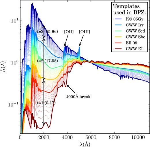
The 66 spectral templates in the rest frame extracted from the extended CWW library. They are used, in equations (7) and (10), to generate the photometry of the PAU mock catalogue. They evolve from Ellipticals (0–17, in red) to Spirals (17–55, in yellow, green and cyan), and finally to Irregulars (55–66, in blue and violet). Wider and deeper curves highlight the five templates used in bpz to compute the photo-z.

After assigning {z, t} values for all galaxies, we also assign them an absolute magnitude M randomly within the range [ − ∞, M_lim(z, t)] following the LF probability distribution in equation (5). Then, the apparent magnitude m₀, in our reference band r_SDSS, is computed from equation (7). The other magnitudes m_j at any band j are obtained through

\begin{eqnarray} m_j = m_0 + 2.5 \log _{10} \left[ {\int ^{\infty }_{0} f_t((1+z)\lambda ) R_0(\lambda )\lambda\, {\rm d}\lambda \over \int ^{\infty }_{0} f_t((1+z)\lambda ) R_j(\lambda )\lambda \rm{d}\lambda } {\int ^{\infty }_{0} R_j(\lambda )\, {\rm{d}\lambda \over \lambda } \over \int ^{\infty }_{0} R_0(\lambda ) {\rm{d}\lambda \over \lambda }}\right],\!\!\!\nonumber\\ \end{eqnarray}

(10)

where R_j(λ) is the response of some PAU band j.

3.2 Noisy magnitudes

The resulting magnitudes are noiseless, so we have to transform them to observed magnitudes by adding a random component of noise as follows:

\begin{equation} m_j \rightarrow m_j + \eta (0,1)\sigma _{m_j}, \end{equation}

(11)

where η(0, 1) is a normal variable and |$\sigma _{m_j}$| the expected magnitude error which is related to the S/N in equation (2) as follows:

\begin{equation} \sigma _{m_j} = 2.5 \log _{10} \left(1 + {1 \over (S/N)_j} \right) . \end{equation}

(12)

Additionally, we add an extra component of noise of size ∼0.022, corresponding to an S/N = 50, in quadrature to σ_m, which takes into account some possible photometric calibration issues. Finally, we obtain the mock catalogue |$\lbrace m_j \pm \sigma _{m_j}, z,t \rbrace$|⁠.

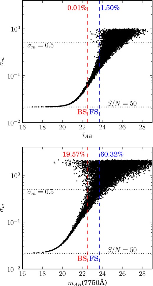
The resulting σ_m versus m scatter plots, in the i BB and the 7750 Å NB, are shown in Fig. 5, where for the sake of clarity we only plot 10 000 randomly selected galaxies. The 7750 Å band is chosen because its central wavelength is very similar to that of the i band. Note, how on both bands σ_m starts being flat at ∼0.022 (the calibration error), and then, at fainter magnitudes, when the sky brightness and the CCD read-out noise become important, it grows and the scatter becomes wider.

Figure 5.

Scatter plots of σ_m versus m for the i BB (top) and the 7750 Å NB (bottom). For the sake of clarity, only 10 000 randomly selected galaxies are plotted. The magnitude limits of the BS (red) and FS (blue) are also plotted as vertical-dashed lines. The bottom dotted line in both plots shows the calibration error (S/N = 50) added in quadrature to σ_m, while the top dotted line shows the threshold where magnitudes are considered as non-observed. The proportions of non-observed magnitudes (σ_m > 0.5) in each sample are also shown at the top with their correspondent colour.

3.3 Bright and faint samples

The PAU survey science will be mostly focused on LSS studies such as cross measurements of redshift space distortions (RSD) and magnification bias (MAG) between two galaxy samples: the bright sample (BS) on the foreground and the faint sample (FS) on the background (see Gaztañaga et al. 2012). The BS should contain galaxies bright enough to have a large S/N in all bands, including the NBs, and, therefore, reach the necessary photo-z accuracy to measure RSD. We see in Fig. 3 that the 5σ limiting magnitudes for the NB are close to 22.5, so we define the BS as all those galaxies with i_AB ≡ m_AB(i) < 22.5. The FS will contain the rest of the galaxies within 22.5 < i_AB < 23.7. The upper limit has been chosen to roughly match the 5σ limiting magnitudes of the BBs (see Fig. 3). We consider that a magnitude is not observed in one band if its correspondent error is σ_m > 0.5. We find that a ∼0.01 per cent of galaxies in the BS are not observed in the i band, with the fraction increasing to ∼1.5 per cent in the FS. Similarly, in the BS ∼19.57 per cent are not observed in the 7750 Å band, increasing to ∼60.32 per cent in the FS (see Fig. 5). This tells us that, while most of the BB information will be present in both samples, the presence of NB information in the FS will be rather limited, degrading considerably the photo-z.

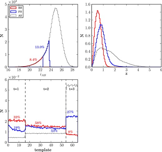
In Fig. 6, we show the resulting distributions of the magnitude i_AB (top left), the true redshift z (top right) and the spectral type t (bottom) of the galaxies in the whole catalogue (black-dotted), the BS (red-solid) and the FS (blue-solid). The magnitude distribution of the whole catalogue has its maximum at ∼25.0, so that the BS and FS are on the brighter tail of the distribution and account for ∼8.4 and ∼13 per cent of the whole catalogue, respectively. However, this also helps both samples to have a very good completeness up to their magnitude limit. We can also see that, while the whole catalogue extends up to z ∼ 5, the BS only goes up to z ∼ 1.5 and the FS up to z ∼ 3. Finally, we see that both BS and FS have a similar proportion of Spiral galaxies (t = 2), ∼55 per cent; however, the BS contains more elliptical galaxies (33 per cent) than the FS (19 per cent), and consequently, the FS contains more irregular galaxies.

Figure 6.

The observed magnitude in the i band (top-left), true redshift (top-right) and spectral type distributions for the whole catalogue (black), the BS i_AB < 22.5 (red) and the FS 22.5 < i_AB < 23.7 (blue). We also show the fraction of the total galaxies in each sample in the magnitude distribution plot, in their corresponding colour. Similarly, we show the proportions of spectral types in each sample. The redshift and type distributions have been normalized.

4 PHOTO-z PERFORMANCE

In this section, we compute the photometric redshifts z_ph of the galaxies in the BS and the FS generated in the previous section and analyse their photo-z performance through different statistical metrics: bias, photo-z precision and outlier fraction. We also apply some photo-z quality cuts (odds cuts) on the results and analyse how the performance improves. We investigate how many galaxies with poor photo-z quality we need to remove in order to achieve the photo-z precision requirements defined in Gaztañaga et al. (2012).

The photo-zz_ph are obtained using the bpz⁴ template-fitting code described in Benitez (2000). It uses Bayesian statistics to produce a posterior probability density function p(z|m_j) that a galaxy is at redshift z when its magnitudes in the different bands j are m_j

\begin{equation} p(z|m_j) \propto \sum _t L(m_j|z,t) \, \Pi (z,t \!\mid\! m) \,, \end{equation}

(13)

where L(m_j|z, t) is the likelihood that the galaxy has magnitudes m_j, if its redshift is z and its spectral type t, and Π(z, t∣ m) is the prior probability that the galaxy has redshift z and spectral type t when its magnitude in some reference band is m. The proportionality symbol is a reminder that p(z|m_j) must be properly normalized in order to be a probability density function. The photometric redshift z_ph of the galaxy will be taken as the position of the maximum of p(z|m_j).

We have modified the bpz code in order to increase its efficiency when estimating photo-z using a large number of NB filters. Instead of estimating the photo-z for each galaxy, the calculations are done in blocks of hundreds of galaxies using linear operations. Details will be presented in Eriksen et al. (in preparation).

4.1 Templates

The likelihood L(m_j|z, t) is generated by comparing the observed magnitudes with the ones that are predicted through a collection of galaxy templates that span all the possible galaxy types t. bpz includes its own template library; however, we use a subset of six templates from the same library used in the previous section for the mock catalogue generation. They are highlighted in Fig. 4 and correspond to the templates with file name: CWW_Ell.sed, Ell_09.sed, CWW_Sbc.sed, CWW_Scd.sed, CWW_Irr.sed and I99_05Gy.sed. Additionally, we also include two interpolated templates between each consecutive pair of the six by setting the bpz input parameter INTERP=2. This results in a total of 16 templates. However, we will see later in Fig. 10 that the number of interpolated templates does not affect much the photo-z performance.

4.2 Prior

An important point of bpz is the prior probability Π(z, t∣m) that helps improve the photo-z performance. Benitez (2000) proposes the following empirical function:

\begin{eqnarray} \Pi (z, t \!\mid\! m)&=&\Pi (t \!\mid\! m) \Pi (z \!\mid\! t, m) \nonumber \\ &&\propto f_t {\rm e}^{-k_t(m-m_0)} z^{\alpha _t}\exp \left\lbrace -\left[ {z \over z_{mt}(m)} \right]^{\alpha _t} \right\rbrace , \end{eqnarray}

(14)

where z_mt(m) = z_0t + k_mt(m − m₀) and m₀ is a reference magnitude, in our case equal to 19 in the i band. Each spectral type t has associated a set of five parameters {f, k, α, z₀, k_m} that determine the shape of the prior. In order to calibrate the prior Π(z, t∣m) and determine the value of these parameters, we construct a training sample consisting of 10 000 galaxies randomly selected from the mock catalogue with i_AB < 24. We only need to know their observed magnitude i_AB in our reference band, their true redshift z_tr and their true spectral type t_tr. Originally, t ranged from 0 to 66 which is the number of templates used to generate the mock catalogue; however, as we did for the LFs galaxy types in the previous section, we group all these galaxy types in three groups: t = 1 (ellipticals), t = 2 (spirals) and t = 3 (irregulars), whose correspondence is 1→(0–17), 2→(17–55) and 2→(55–66). From now on, we will use t for either the 66 templates or these three galaxy-type groups. Finally, we fit equation (14) to the training sample and recover the prior parameters. We show the resulting values in Table 4. Parameters f₃ and k₃ do not appear in the table because Π(t = 3∣m₀) is deduced by imposing the proper normalization. In Fig. 7, we show a comparison between the fitted curve and the actual distribution of the prior. Π(t | m) on the left and Π(z | t, m) on the right are shown at different magnitudes (rows) from i_AB = 19, the reference magnitude, to i_AB = 24. On the one hand, the fitted Π(t|m) agrees by definition with the actual distribution at the reference magnitude (top row), since we use those values as a starting point. However, at higher magnitudes a significant mismatch appears for the spiral and irregular galaxies. This is related to the fact that the k parameters, which control the migration of galaxies from one spectral type to another across magnitude, are positive definite. With this, elliptical and spiral galaxies should turn to irregulars as the magnitude increases. However, in Fig. 7 we observe that actually the spiral abundance grows slightly before starting to decrease at m ∼ 21, and this forces the fit to k₂ = 0. Consequently, elliptical galaxies migrate directly to irregulars, causing a mismatch on the pace of growth of this galaxy-type abundance. On the other hand, the fit of Π(z|t, m) is particularly good for Ell and Sp galaxies at higher magnitudes (the eight bottom-left panels on the right plot of Fig. 7), but for Irr and magnitudes close to the 19 (the reference magnitude) it is less accurate.

Table 4.

The resulting values of the prior parameters obtained by fitting (14) to a subset of 10 000 randomly selected galaxies from the BS and FS together. The three galaxy types t = 1, 2, 3 are the same that were defined in Section 3 for the LFs. f₃ and k₃ do not appear because Π(t = 3∣m₀) is deduced by normalization.

t	f	k	α	z0	km
1	0.565	0.186	2.456	0.312	0.122
2	0.430	0.000	1.877	0.184	0.130
3	–	–	1.404	0.047	0.148

Figure 7.

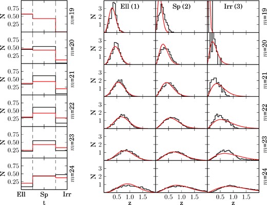
Left: comparison between the fitted Π(t|m) prior (red) of equation (14) and the actual distribution (black). Right: the same for Π(z|t, m). We only differentiate between three galaxy types t (as we did for the LFs in Section 3): 1 = Elliptical, 2 = Spiral and 3 = Irregular. Rows correspond to i_AB magnitude bins of width Δm = 0.2 centred at values from m = 19 to 24 in steps of 1. All curves have been normalized. Resulting prior parameters are on Table 4.

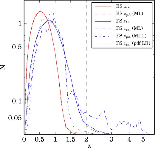
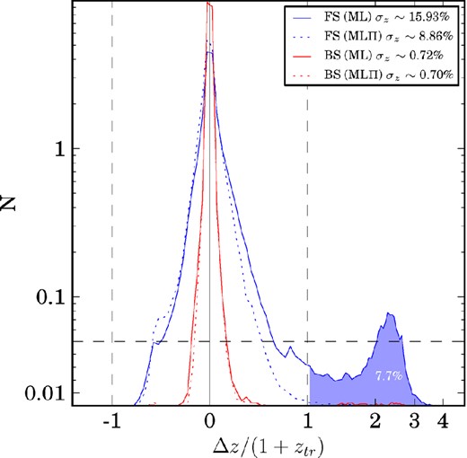
In Fig. 8, we show a comparison between the z_tr (solid) and z_ph (discontinuous) distributions for the BS and the FS. For the sake of clarity, the x- and y-axes have been set to be linear below z = 2 and N = 0.1, respectively, and logarithmic elsewhere. Dashed lines correspond to z_ph obtained by maximizing only the likelihood L(m_j|z, t) in (13). This gives a z_ph distribution in the BS very close to the actual, while in the FS a residual long tail towards much higher redshift (z ∼ 5) appears. In Fig. 9, we show the equivalent Δz/(1 + z_tr) distributions, where Δz ≡ z_ph − z_tr. Once again, the x- and y-axes have been set to be linear below |Δz|/(1 + z_tr) = 1 and N = 0.05, respectively, and logarithmic elsewhere. Note that the tail is also present on the right-hand side of the blue curve. If we define as catastrophic outliers those galaxies with |Δz|/(1 + z_tr) > 1, we find that they account for ∼7.7 per cent in the FS (the blue region under the curve) and ∼0.2 per cent in the BS. Catastrophic outliers are typically caused by degeneracies in colour space, which cause confusions in the template fit and result in a much larger |Δz|. The blue-dotted line in Fig. 9 shows that when the prior is included almost all of the catastrophic outliers in the FS are removed, leaving only a small fraction of ∼ 0.1 percent. We see in Fig. 8 that the z_ph distribution after applying the prior (blue dot–dashed) decays at high redshifts faster than the z_tr distribution. This is because we are only using the maximum of p(z|m_j) for the z_ph value. If we use the whole probability density function (pdf) information (blue-dotted line), the resulting z_ph distribution is much closer to the true. Defining the photo-z precision σ_z as half of the symmetric interval that encloses the 68 per cent of the Δz/(1 + z_tr) distribution area around the maximum, we find that σ_z almost does not change in the BS (0.72–0.70 per cent), while it improves by a factor of ∼1.8 in the FS by going from σ_z ∼ 16 to ∼ 8.86 percent when adding the prior. In the BS sample, the likelihood function is already narrow enough, thanks to the constraining power of the NBs, and, hence, the prior has very limited impact on the final result.

Figure 8.

Comparison between the true redshift (solid) and the photo-z (discontinuous) distributions for the BS (red) and FS (blue). For the sake of clarity, we have set the x- and y-axis scales to be linear below the black dashed lines and logarithmic above them. All distributions have been normalized to equal area. Dashed lines correspond to the z_ph obtained by maximizing only the likelihood L(m_j|z, t) (ML) of (13), the dash–dotted line includes the prior (MLΠ) and the dotted line corresponds to the case when all the p(z|m_j) are stacked (pdf LΠ).

Figure 9.

Δz/(1 + z_tr) distributions, where Δz ≡ z_ph − z_tr, for the BS (red) and FS (blue) with the z_ph obtained by maximizing only the likelihood L(m_j|z, t) (ML) (solid) or when also including the prior (MLΠ) (dotted). Photo-z precision σ_z values, defined as half of the symmetric interval that encloses the 68 per cent of the distribution area around the maximum, are shown for each case in the legend. The x-axis scale is linear between the two dashed vertical lines and logarithmic on the sides. Similarly, the y-axis is linear below the horizontal dashed line and logarithmic above. The prior makes no difference on the BS, but in the FS it removes the long tail (blue region) of catastrophic outliers (|Δz|/(1 + z_tr) > 1) that accounts for a ∼ 7.7 percent of the sample. This reduces σ_z by a factor of ∼1.8.

4.3 Performance versus template interpolation

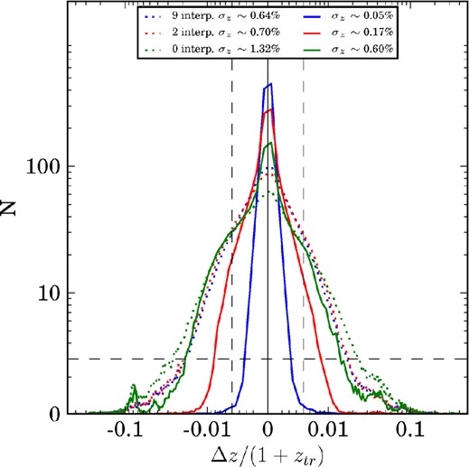
At this point, we want to explore how the number of interpolated templates used in bpz changes the z_ph performance. In Fig. 10, we show the Δz/(1 + z_tr) distribution only for the BS when we use: 9 (blue), 2 (red) and 0 (green), interpolated templates. Solid lines correspond to the z_ph obtained when the input magnitudes are noiseless (without applying equation 11), while dotted lines include the noise. The σ_z of each distribution is shown in the legend. We see that, while for noiseless magnitudes the number of interpolated templates has a significant impact on the width of the distributions and so, on their σ_z, which gets worse by a factor of ∼3 at each step, for noisy magnitudes these differences are smaller. In fact, going from 9 to 2 interpolated templates the differences are negligibly small and going from 2 to 0 interpolations the difference is less than a factor of 2.

Figure 10.

The Δz/(1 + z_tr) distributions for the BS using different number of interpolated templates in bpz, when input magnitudes are noiseless (solid) and when they are noisy (dotted). Photo-z precision σ_z values for each case are shown on the legend. The x-axis scale is linear between the two dashed vertical lines and logarithmic on the sides. Similarly, the y-axis is linear below the horizontal dashed line and logarithmic above.

4.4 Performance versus odds

Photo-z codes, besides returning a best estimate for the redshift, typically also return an indicator of the photo-z quality. It can be simply an estimation of the error on z_ph, or something more complex, but the aim is the same. In bpz, this indicator is called odds, and, it is defined as

\begin{equation} odds = \int ^{z_{{\rm ph}}+\delta z}_{z_{{\rm ph}}-\delta z}p(z|m_j)\,\rm{d}z \,, \end{equation}

(15)

where δz determines the redshift interval where the integral is computed. Odds can range from 0 to 1, and the closer to 1, the more reliable is the photo-z determination, since p(z|m_j) becomes sharper and most of its area is enclosed within z_ph ± δz. We choose δz = 0.0035 in the BS and 0.05 in the FS, which is close to the expected σ_z in these samples for the PAU Survey (see the σ_z plots in Fig. 11). A bad choice of δz could lead to the accumulation of all odds close to either 0 or 1. Since odds are a proxy for the photo-z quality, we should expect a correlation between the odds and |Δz| in the sense that higher odds should correspond to lower |Δz|.

Figure 11.

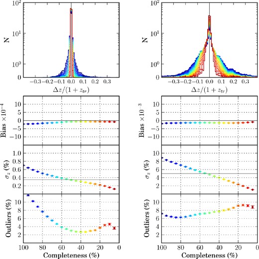
Top: Δz/(1 + z_tr) distributions for the BS (left) and the FS (right) at different photo-z quality cuts whose completeness, shown in a colour degradation, range from 100 per cent (bluest) to 5 per cent (reddest) in 5 per cent steps. On the bottom and by rows: the bias (median), the photo-z precision (σ_z) and the 3σ-outlier fraction of the distributions at the top as a function of the completeness. The colours of the points match the colours in the distributions. Note that the vertical scale in the bias and the σ_z panels changes by an order of magnitude between the two samples. The black-dashed horizontal lines on the σ_z panels show the photo-z precision requirements defined in Gaztañaga et al. (2012): σ_z < 0.35 per cent (BS) and <5 per cent (FS).

At the top of Fig. 11, we show the Δz/(1 + z_tr) distributions in a colour degradation for subsets of the BS (left) and the FS (right) with increasingly higher cuts on the odds parameter. In fact, the exact odds values are quite arbitrary, since they depend on the size of δz. Therefore, we have translated these odds cuts into the fraction of the galaxy sample remaining after a certain cut has been applied, in such a way that the bluest curve corresponds to 100 per cent completeness while the reddest corresponds to 5 per cent completeness, with 5 per cent steps. We can clearly see how the harder are the odds cuts, the narrower and peaky become the distributions in both samples. On the bottom plots of the same figure, we show how some statistical metrics of these distributions (the bias (median), the photo-z precision (σ_z) and the 3σ-outlier fraction) depend on each odds cut of completeness given in the x-axis. The 3σ-outlier fraction is defined as the fraction of galaxies with |Δz|/(1 + z_tr) > 3σ_z. For the sake of clarity, each point has been coloured as its correspondent distribution. Errors are computed by bootstrap (Efron 1979) for the bias and σ_z, and, by computing the σ₆₈ of a binomial distribution with mean n_outlier/N for the outlier fraction. As we expected, σ_z decreases as the odds cuts get more stringent. In the BS (left), it goes from ∼0.7 per cent at 100 per cent of completeness to ∼0.1 per cent at 5 per cent, and in the FS (right), from ∼9 to ∼1 per cent. The photo-z precision requirements, as defined in Gaztañaga et al. (2012), are σ_z < 0.35 per cent in the BS and σ_z < 5 per cent in the FS. They are fulfilled when ∼50 per cent of each catalogue is removed. We find a very small bias of a few per cent of σ_z in both samples towards negative Δz values. It practically vanishes when high odds cuts are applied. The 3σ-outlier fraction in the BS starts at ∼13 per cent, drops to ∼3 per cent at ∼40 per cent completeness and then, starts increasing again up to ∼4.5 per cent at ∼10 per cent completeness. Therefore, we deduce that the gain on σ_z with the odds cut occurs basically through the cleaning of outliers. However, in the FS, even if σ_z decreases with the odds cuts, the outlier fraction increases from ∼7 to ∼9 per cent at ∼15 per cent completeness.

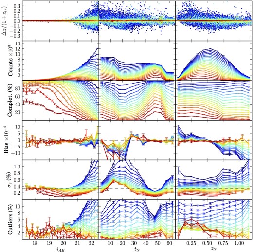
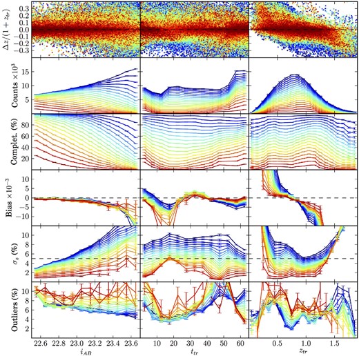
On the last three rows of plots in Figs 12 (BS) and 13 (FS), we show how these statistical metrics depend on the observed magnitude i_AB (left), the true spectral type t_tr (centre) and the true redshift z_tr (right), after each photo-z quality cut shown in Fig. 11 in the same colour. In the first three rows and by order, we also show the scatter plot Δz/(1 + z_tr), the number of galaxies and the completeness after the same photo-z quality cuts with respect to the same variables (i_AB, t_tr,z_tr) on the x axis.

Figure 12.

Statistics showing the PAU-BS photo-z performance as a function of the observed i_AB magnitude (left), true galaxy type t_tr (centre) and true redshift z_tr (right). In the first row, we show the scatter Δz/(1 + z_tr). Then, in a descending order of rows, we show the number of galaxies, the completeness, the bias (median), the photo-z precision (σ_z) and the 3σ-outlier fraction for all the odds cuts shown in Fig. 11 (same colour). Also as in Fig. 11, the black-solid horizontal lines on the σ_z panels show the photo-z precision requirement defined in Gaztañaga et al. (2012).

Figure 13.

Statistics showing the PAU-FS photo-z performance in the same layout as in Fig. 12.

In the BS (Fig. 12), we can see that the low photo-z quality galaxies (blue points in the scatter plot) are mostly faint galaxies with i_AB > 21, the magnitude where the noise coming from the sky brightness plus the CCD read-out starts to be comparable to the Poisson noise in signal. This is reflected in Fig. 5 as a turning point on the slope of the σ_m versus m_AB scatter. In fact, these galaxies represent most of the outliers and the principal source of bias seen in Fig. 11. As the odds cuts are applied, these bad photo-z faint galaxies are removed. The odds cut removes the bias, reduces σ_z from ∼2.2 to ∼0.35 per cent and the outlier fraction from >10 to ∼1 per cent at magnitudes close to the limit i_AB = 22.5. Looking at the scatter plots of the next two columns in Fig. 12, we realize that these low-odds galaxies at faint magnitude are spread out over the whole t_tr and z_tr ranges. Moreover, after the hardest odds cut, only galaxies of types t ∼ 0 (elliptical) and t ∼ 50 (irregular) survive and the mean of z_tr is shifted from ∼0.6 to ∼0.4. The worst bias, σ_z and outlier fraction are obtained for spiral galaxies (t ∼ 10–30). The odds cuts mitigate these results, but even after applying them, spiral galaxies still have the worst bias and σ_z. The worst bias is located at low and high z_tr, with opposite sign and it is largely reduced with the odds cuts. The value of σ_z gets flatter over all z_tr as the odds cuts are harder.

Regarding the z_ph precision requirement σ_z < 0.35 per cent (black solid horizontal line), we find that, when no odds cut is applied, it is achieved only for galaxies with i_AB < 21 and galaxy type around t ∼ 50 (irregulars). However, it is not fulfilled at any z_tr. Once we apply a 50 per cent completeness odds cut, which gives an overall σ_z equal to the requirement, as we saw in Fig. 11, the requirement is fulfilled in all the i_AB and z_tr ranges. Only for spiral galaxies, the requirement is not fulfilled even after the hardest odds cut. Originally, in Benítez et al. (2009), it was assumed that elliptical galaxies (or rather luminous red galaxies) yield the best photo-z precision in the PAU Survey, with the NBs tracking the ∼4000 Å break spectral feature (Fig. 4). This is partially true, since we actually see that elliptical galaxies give better σ_z than spirals, but our analysis shows that in fact irregulars with t ∼ 50 give the best photo-z performance. Before any odds cut, their photo-z precision is almost twice better than the requirement. Probably, this is due to the fact that, in contrast to elliptical galaxies were a single spectral feature is tracked, irregulars have the two emission lines [O ii] ∼3737 Å and [O iii] ∼5000 Å (Fig. 4) with intrinsic widths narrower than the width of the NB filters.

In the FS (Fig. 13), we see that the scatter of Δz/(1 + z_tr) is much larger, as expected from the wider histograms in Fig. 11. However, a wider but still tight core close to Δz = 0 with high photo-z quality (red points) remains. We recognize behaviours similar to those in the BS in most aspects of the z_ph performance, although they are substantially larger. For example, the highest magnitude as well as lowest and highest z_tr galaxies are the most biased. The odds cuts also mitigate this bias, but a residual bias of opposite sign persists at the extremes of z_tr. Spiral galaxies (t ∼ 10–30) are also the ones with the highest bias, and the odds cuts even aggravates this. We also see that elliptical (t ∼ 0) and irregular (t > 50) galaxies are initially biased, but, in contrast to spirals, the odds cuts help to reduce the bias. Unlike in the BS, σ_z increases along all the magnitude range since at those magnitudes the noise from the sky brightness dominates over the signal (Fig. 5). However, we see that the slope of the σ_z increase is smaller the harder the odds cuts. This is because the gain in photo-z precision is at the expense of keeping only brighter galaxies each time. The mean i_AB magnitude goes from ∼23.2 to ∼22.8 with the odds cuts, and the shift in the z_tr mean is from ∼0.86 to ∼0.81. Unlike in the BS, we see that the best σ_z is obtained at the extremal spectral types: t ∼ 0 (elliptical) and t ∼ 66 (irregular). However, once the hardest odds cuts are applied, irregular galaxies with t ∼50 are again the once with the best σ_z. In fact, the hardest odds cuts also remove all spiral galaxies. Note that the large bias seen at the extremes of z_tr make σ_z take values much larger at these redshifts. The photo-z precision requirement, σ_z < 5 per cent, is fulfilled when the odds cut of 50 per cent completeness is applied up to magnitude ∼23.1, for all galaxy types except spirals, and at the z_tr interval from ∼0.4 to ∼1.3. As we already saw in Fig. 11, the 3σ-outlier fraction grows with the odds cuts. In general, its values are higher where σ_z is lower, since the outliers criterion becomes more stringent.

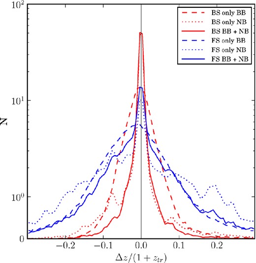
4.5 NBs versus BBs

We want to quantify the improvement that the NB bring to the photo-z performance. For this purpose, we run bpz on the BS and the FS using the NB and the BB separately. Then, in Fig. 14 and Table 5, we compare results between these runs and also with the original ones when the BB and the NB are used together (BB+NB). Fig. 14 shows normalized Δz/(1 + z_tr) distributions for the BS (red) and the FS (blue) using only the BB (dashed), only the NB (dotted) and both together BB+NB (solid). We see that the resulting distributions when using only BB (dashed) show overall shapes close to Gaussian with perhaps larger tails on both sides. However, when the NBs are also included (solid) the peaks of the distributions become clearly sharper. This is more noticeable in the BS than in the FS, because the non-observed condition (σ_m < 0.5) defined in Section 3 implies that most of the NB are not used in the photo-z determination for the FS. Table 5 shows bias (median), σ_z (σ₆₈) and 3σ-outlier fraction of each distribution. σ_z in the BS is reduced ∼4.8 times going from ∼3.34 to ∼0.7 per cent when the NB are included, while the improvement is much less significant in the FS. We also see that bias is reduced by an order of magnitude when the NB are included in both samples. On the contrary, the outlier fraction increases, but as mentioned, this is due to the fact that improvements on σ_z penalize the outlier fraction. On the other hand, we see that using NB alone slightly degrades all metrics in the BS and the FS, except the outlier fraction in the FS which is improved for the same reason. In fact, σ_z in the FS gets almost twice worse than when only using BB or BB+NB. It seems that in the FS NB by themselves only help the bias, while if they are used together with the BB, the improvement also extends to σ_z. These results are in qualitative agreement with previous findings using photometric systems mixing BB and NB, such as those in Wolf, Meisenheimer & Rser (2001).

Figure 14.

Normalized Δz/(1 + z_tr) distributions for the BS (red) and the FS (blue) using only BB (dashed), only NB (dotted) or both together BB+NB (solid). Bias, σ_z and 3σ-outlier fraction of each distribution are shown in Table 5.

Table 5.

Bias (median), σ_z (σ₆₈) and 3σ-outlier fraction when using only BB, only NB or both together BB+NB for the bright and faint samples.

	BS
	BB	NB	BB + NB
Bias× 10−4	−31.64	−3.31	−2.18
σz (per cent)	3.34	0.83	0.70
Outliers (per cent)	4.41	18.19	13.28
	FS
	BB	NB	BB + NB
Bias× 10−4	−152.66	−41.19	−19.01
σz (per cent)	9.38	16.17	8.86
Outliers (per cent)	6.79	4.90	7.18

4.6 Impact of the photo-z on the clustering

We want to study the impact of the PAU photo-z performance on the measurements of angular clustering. In Gaztañaga et al. (2012), it is shown that galaxy cross-correlation measurements |$\bar{\omega }_{ij}$| between two photo-z bins i and j are related to their cross-correlation between real redshift bins ω_ij as

\begin{equation} \bar{\omega }^{{\rm A}\times {\rm B}}_{ij} = \sum _{kl} r^{\rm A}_{ik} \omega ^{{\rm A} \times {\rm B}}_{kl} r^{\rm B}_{jl} = r_{\rm A} \omega ^{{\rm A} \times {\rm B}} r^{\rm T}_{\rm B}, \end{equation}

(16)

where r_ij is called the migration matrix and gives the probability that a galaxy observed at the photo-z bin i will be actually at the true redshift bin j, while A and B denote different galaxy samples. We compute the migration matrices from the PAU photo-z simulations and show them in Fig. 15 for the BS (top) and the FS (bottom) in photo-z bins of width 0.014(1 + z), which is four times the photo-z precision σ_z in the BS once the photo-z quality cut that leaves a 50 per cent completeness is applied. Note that the matrices are normalized row-wise by definition. The FS migration matrix has quite a thick diagonal, i.e. around z_tr ≃ 1 the width is Δz ≃ 0.1 for ≃10 per cent probabilities and Δz ≃ 0.4 for ≃1 per cent. There are also outliers going from very large true redshifts z_tr ≃ 1.8 to lower photo-z redshifts and some from low true redshifts up to z_ph ≃ 1. The BS has a thinner diagonal with Δz < 0.04 at ≃1 per cent probability and with fewer outliers. These values are of course in agreement with previous results in Figs 9 and 11.

Figure 15.

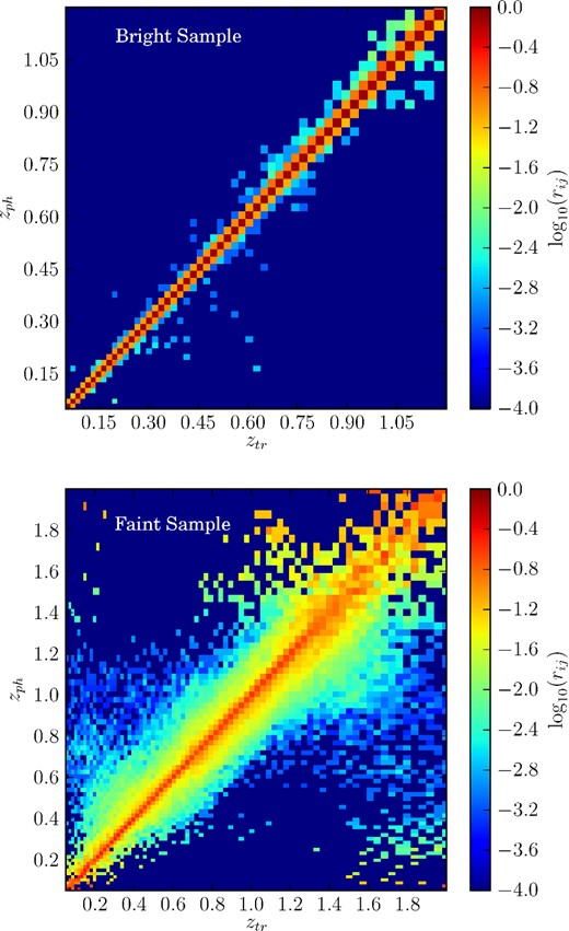
The resulting migration matrices r_ij from the PAU photo-z simulations after applying the photo-z quality cut that leaves 50 per cent completeness. The top plot corresponds to the BS and the bottom plot to the FS. For a higher contrast and clarity, we plot the logarithm of the matrix values. These matrices give the probability that a galaxy observed at the photo-z bin i, will be actually at the true redshift bin j. The bin widths are 0.014(1 + z), four times the photo-z precision expected in the BS.

To illustrate how these matrices affect angular clustering measurements, we use a simple model to predict ω_ij at an arbitrary reference angular scale, θ, of 1 arcmin. We include intrinsic galaxy clustering and weak lensing magnification:

\begin{eqnarray} w_{ij} &=& w_{G_iG_j}+ w_{G_i\mu _j} + w_{\mu _i G_j}+ w_{\mu _i\mu _j} \nonumber \\ w_{G_iG_j} &=& b_ib_j \int {\rm d}z_1{\rm d}z_2 \, \, \phi _{G_i}(z_1) \, \phi _{G_j}(z_2) \, \, \xi (r_{12}) \nonumber \\ w_{G_i\mu _j} & =& b_i \alpha _j \int {\rm d}z_1 {\rm d}z_2 \, \,\phi _{G_i}(z_1) \, p_{\mu _j}(z_2) \, \, \xi (r_{12}) \nonumber \\ w_{\mu _i\mu _j} & =& \alpha _i \alpha _j \int {\rm d}z_1 {\rm d}z_2 \, \, p_{\mu _i}(z_1) \, p_{\mu _j}(z_2) \, \, \xi (r_{12}), \end{eqnarray}

(17)

where ξ(r₁₂) is the non-linear matter two-point correlation between the positions of two galaxies separated in 3D space by r₁₂ = r₂ − r₁, where the angular separation between r₁ and r₂ is fixed to be the reference angle (i.e. θ = 1 arcmin), while the radial separation is integrated out via z₁ and z₂. We have that |$\phi _{G_i}(z)$| is a top-hat distribution for galaxies in the redshift bin i and |$p_{\mu _j}(z)$| is the efficiency of weak lensing effect for lenses at z and sources at z_j (following the notation in Gaztañaga et al. 2012). The coefficient b_i is the effective galaxy bias at z_i and α_j ≡ 2.5s_j − 1 is the amplitude of the weak lensing magnification effect (with s_j the slope of the galaxy number counts at the flux limit of the sample at z_j). The first equation above has four terms corresponding to galaxy–galaxy (intrinsic clustering), galaxy–magnification, magnification–galaxy and magnification–magnification correlation. In our test, we use α_i = 1 and b_i = 1 to generate the starting point for ω_ij. We then apply the following transformation:

\begin{eqnarray} \omega ^{{\rm B}\times {\rm B}}_{ij} \rightarrow b_{{\rm B}}(z_i)b_{{\rm B}}(z_j)\omega _{ij} \end{eqnarray}

(18)

\begin{eqnarray} \omega ^{{\rm F}\times {\rm F}}_{ij} \rightarrow b_{{\rm F}}(z_i)b_{{\rm F}}(z_j)\omega _{ij} \end{eqnarray}

(19)

\begin{eqnarray} \omega ^{{\rm B}\times {\rm F}}_{ij} \rightarrow b_{{\rm B}}(z_i)b_{{\rm F}}(z_j)\omega _{ij} \end{eqnarray}

(20)

depending on which galaxy samples we are cross-correlating (FS or BS), where

\begin{eqnarray} b_{{\rm B}}(z_i) &=& 2 + 2 (z_i - 0.5) \end{eqnarray}

(21)

\begin{eqnarray} b_{{\rm F}}(z_i) &=& 1.2 + 0.4 (z_i - 0.5) \end{eqnarray}

(22)

are the biases in the BS and FS, respectively, in the photo-z bin i (at mean redshift z_i). This corresponds to using linear bias for the intrinsic correlation (as in Gaztañaga et al. 2012) and some particular evolving slope (s_i ∼ 1) for the magnification cross-correlations. In Fig. 16, we show |$\omega ^{{\rm B}\times {\rm B}}_{ij}$| (left), |$\omega ^{{\rm F}\times {\rm F}}_{ij}$| (middle) and |$\omega ^{{\rm B}\times {\rm F}}_{ij}$| (right) before (top) and after (bottom) being transformed by the migration matrices r_ij in Fig. 15 through equation (16). Note that for the B × B and F × F cases, the correlations matrices are symmetrical. Also note that the redshift ranges in both samples are different, so that the B × F correlation matrix is not squared.

Figure 16.

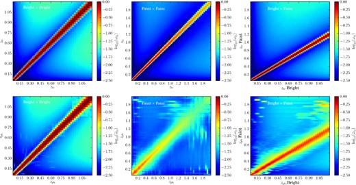
Top panels show the angular auto (diagonal) and cross- (off-diagonal) correlations ω_ij at 1 arcmin between the true redshift bins i and j of the BS (left), the FS (middle) and the crossing of both of them (right). Bottom plots show the same correlations but measured with photo-z bins, which can be computed by using equation (16) with the migration matrices in Fig. 15. The bin widths are 0.014(1 + z), four times the photo-z precision expected in the BS.

In the top panels, we can see the intrinsic galaxy–galaxy clustering in the diagonal of the matrix, which has an amplitude of order unity and decreases rapidly to zero for separated redshift bins. The galaxy–magnification correlation appears as a diffused off-diagonal cloud with an amplitude <0.05 (clear colours). The magnification–magnification contribution is negligible. In the bottom panel, we see the effect of the photo-z migration. The diagonal (auto-correlations) becomes thicker and diluted. The off-diagonal galaxy–magnification cloud becomes more diffused, especially for the FS. The cross-correlation F × B produces results that are intermediate between B × B and F × F.

We can invert the migration matrices to go from the bottom panels (which are the observations |$\bar{\omega }^{{\rm A}\times {\rm B}}$|⁠) to the top panels (i.e. true correlations ω^{A × B}) by inverting equation (16):

\begin{equation} \omega ^{{\rm A} \times {\rm B}} =r_{\rm A}^{-1} \bar{\omega }^{{\rm A}\times {\rm B}} \left(r^{\rm T}_{\rm B}\right)^{-1}. \end{equation}

(23)

This should work perfectly well if we can calibrate the r_ij matrices properly. For a large fiducial survey with about 5000 deg², we need about ≃1 per cent accuracy in r_ij (Gaztañaga et al. 2012). In practice, the accuracy of the above reconstruction can be used to put requirements on the photo-z calibration.

5 OPTIMIZATION OF THE PAU FILTER SET

In this section, we want to explore how the photo-z performance changes under variations of the PAU NB filter set.

5.1 NB filter set variations

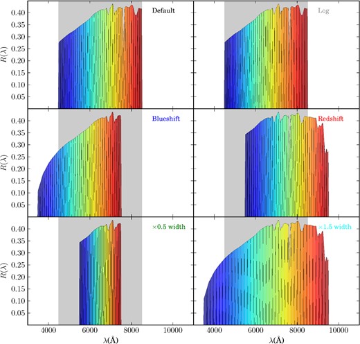
We study five variations of the original NB filter set whose response is shown in Fig. 17. All the variations conserve the number of filters. In the order that appear in Fig. 17, the proposed filter sets are:

• Default: this is the default filter set already shown in Fig. 2.

• Log: in this filter set, band widths increase in wavelength logarithmically, so that they fulfil λ₀/Δλ = const., where Δλ is the width of the rectangular part of the band (without taking into account the lateral wings) and λ₀ is the central wavelength of the band. We impose the overall wavelength range covered by the set of bands to be the same as for the Default filter set. Given that the total number of bands is kept at 40, we obtain that the bluest filter has a width of 97 Å, while the reddest is 159 Å wide. The reason for this filter set is that, when spectra are redshifted, their spectral features are moved to redder wavelengths, but also their widths are stretched as Δλ′ = (1 + z)Δλ. If the photo-z determination depends strongly on the tracking of any spectral feature, such as the 4000 Å break in elliptical galaxies, a filter set like Log will continue to enclose the same part of the spectral feature in a single feature independently of how redshifted is the spectrum.

• Blueshift: this is the same as the Default filter set, however bands have been shifted 1000 Å towards bluer wavelengths. We expect to get better photo-z performance at low redshift and for late-type galaxies. The down side of this filter set is that the overall response turns out to be very inefficient in the ultraviolet zone (middle-left of Fig. 17), like it was for the u band.

• Redshift: this is the same variation as before but shifting bands 1000 Å towards redder wavelengths. We expect to get better photo-z performance at high redshift and for early-type galaxies. This filter set does not suffer from the problem of the ultraviolet, so its band responses are much more uniform over the covered range (middle-right of Fig. 17). On the other hand, the sky brightness on this region is higher.

• ×0.5 width: this is a filter set whose band widths are half of the Default ones. Lateral wings are also reduced to half of their size, from 25 to 12.5 Å, in order to avoid an excessive overlap between adjacent bands. We expect to improve the photo-z precision, at least for galaxies with good S/N ratio on their photometry. The down side of this filter set is that, since the number of bands is kept, the overall wavelength range covered is also reduced by a half. We choose it to be centred with respect to the Default, so that it covers from 5500 to 7500 Å, roughly spanning only from the bluest filter of the Redshift set to the reddest of the Blueshift set. This can lead to a degradation of the photo-z at very low and high redshift, although the BBs may attenuate this effect.

• ×1.5 width: this is a filter set whose band widths are 1.5 times wider than the Default ones. Because of this, we expect a significant degradation of the photo-z precision for galaxies with good S/N ratio on their photometry. However, the increase in S/N may help. Moreover, the covered wavelength range also increases by 50 per cent. We choose the new range to be centred with respect to the Default set, so that it covers from 3500 to 9500 Å, roughly from the bluest edge of the Blueshift set to the reddest edge of the Redshift set, so we expect to see a more uniform photo-z performance over the whole redshift range.

Figure 17.

On the top left, the original PAU NB filter set (same as in Fig. 2). The rest are the five variations to be compared in terms of photo-z performance. Greyed areas show the covered wavelength range by the Default filter set. In descending order from left to right we have: the Log filter set with the same overall range as the Default but with band widths that increase logarithmically; the Blueshift filter set, which is the same as the Default but with the bands shifted 1000 Å towards bluer wavelengths; the Redshift filter set which is the same as Default but shifted towards redder wavelengths; the ×0.5 width filter set whose band widths are half those of the Default ones; and the ×1.5 width filter set whose bands are 1.5 times wider. The overall wavelength ranges of these last two set-ups are chosen to be centred respect to the range of the Default set.

We generate magnitudes for each filter set band as described in Section 3 using the same exposure times per NB filter tray and BB as in the Default filter set. We do not try to optimize the exposure times for each filter set. The aim of this study is to see how, in spite of this, the photo-z performance changes. Once the new photometric mock catalogues are created, they are also split into a BS (i_AB < 22.5) and FS (22.5 < i_AB < 23.7). We run bpz on each catalogue using the same settings as for the Default filter set. There is no need to calibrate a different prior for each filter set, since the prior was initially calibrated on the BB i, which is shared by all these filter sets. Photo-z quality cuts resulting in an overall completeness of ∼50 per cent are applied in all cases.

5.2 Global photo-z performance

Global photo-z performance results for each filter set are shown in Table 6, using the same metrics as in Section 4: bias (median), σ_z (σ₆₈) and the 3σ-outlier fraction. We find that the ×0.5 width set gives the best bias (it completely vanishes), and σ_z (∼6 per cent better than Default) in the BS, while in the FS it is the Redshift set which gives the best bias (∼54 per cent better) and the ×1.5 width set which gives the best σ_z (∼18 per cent better). On the other hand, the ×1.5 width set gives the worst bias (a factor of 4.6 worse) and σ_z (∼32 per cent worse) in the BS, while in the FS it is the Blueshift set which gives the worst bias (a factor of 2.4 worse) and the ×0.5 width which gives the worst σ_z (∼46 per cent worse). Regarding the outlier fraction, its direct comparison is trickier since it depends on the value of σ_z. Even so, we see that in the BS the Log set gives the best value, while in the FS the ×0.5 width set gives the worst.

Table 6.

Global photo-z performance results for each filter set shown in Fig. 17. Photo-z performance is characterized through the three metrics: bias (median), σ_z (σ₆₈) and the 3σ-outlier fraction. Photo-z quality cuts resulting in a 50 per cent overall completeness are applied in all cases. We show results for the BS and FS.

	Bias	σz (per cent)	Outliers (per cent)
Default BS	−0.71 × 10−4	0.34	3.02
Default FS	−1.33 × 10−3	4.73	7.36
Blueshift BS	−2.11 × 10−4	0.38	3.23
Blueshift FS	−3.11 × 10−3	5.19	7.05
Redshift BS	−0.74 × 10−4	0.35	3.31
Redshift FS	−0.65 × 10−3	4.99	7.21
Log BS	−0.69 × 10−4	0.35	2.80
Log FS	−1.46 × 10−3	4.73	7.43
×1.5 width BS	−3.18 × 10−4	0.45	3.00
×1.5 width FS	−2.76 × 10−3	3.87	7.76
×0.5 width BS	−0.00 × 10−4	0.32	5.22
×0.5 width FS	−0.99 × 10−3	6.91	5.52

The general conclusions are that the Log set gives almost the same photo-z performance as the Default set, with a slight increase of 3 per cent in σ_z in the BS. Therefore, we see that the logarithmic broadening of the band widths does not provide any global improvement. On the other hand, and as we expected, if the S/N ratio in the photometry is good enough, the narrower the bands, the better the photo-z performance results. On the other hand, wider bands are the ones that give better photo-z precision in the FS, because there are more bands that pass the cut σ_m < 0.5 introduced in Section 3.

5.3 Results as a function of i_AB, t_tr and z_tr

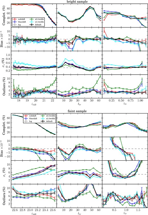
In Fig. 18, we show plots similar to those in Figs 12 and 13 with the photo-z performance metrics as a function of i_AB, t_tr and z_tr for the BS (top) and the FS (bottom) when using the different filter sets of Fig. 17. Black curves correspond to the photo-z results of the Default filter set when the 50 per cent completeness photo-z quality cut is applied, and we will treat them as the reference results. The rest of the curves in different colours correspond to the variations of the Default filter set. As a general trend, we see that these curves do not deviate much from the reference. Even so, we will discuss each case separately.

Figure 18.

Photo-z performance metrics using the different filter sets shown in Fig. 17. Rows: completeness after applying a photo-z quality cut leading to a 50 per cent global completeness; bias (median); σ_z (σ₆₈) and 3σ-outlier fraction, as a function of i_AB, t_tr and z_tr (columns), in the BS (top) and the FS (bottom).

In the BS, we see that redshifting the bands (red curves) slightly degrades the completeness at low magnitudes up to i_AB < 21.5. As was expected, all the metrics also degrade at low z_tr. In contrast, blueshifting the bands (blue curves) shows the opposite behaviour, a degradation of all the metrics at high z_tr. This is due to the lack of coverage at blue and red wavelengths, respectively, of each filter set, as we have already mentioned before. Something similar happens for the ×0.5 width set, where band widths, and consequently the covered wavelength range, is reduced by a half (green curve). The resulting photo-z performance is worse at both low and high z_tr. However, the photo-z precision σ_z is slightly better at intermediate redshifts (0.15 < z_tr < 0.5), for spiral galaxies (10 < t_tr < 30) and at bright magnitudes (i_AB < 20.5). Increasing the band width by a factor of 1.5 (cyan curve) does not result in an improvement in any case. Bias and σ_z degrade all over the range of the three variables, i_AB, t_tr and z_tr. This is in full agreement with the results shown in Table 6, where this filter set was seen as giving the worst photo-z performance. Also in agreement with Table 6, we see that the Log filter set practically does not introduce any change from the Default filter set.

In the FS, we do not observe big differences between the completeness curves, but for example the Blueshift filter set shows slightly lower completeness for elliptical galaxies than for irregulars, unlike the Redshift and ×0.5 width filter sets, which show the opposite behaviour. In the z_tr range, we also recognize similar behaviours as in the BS, as for example the fact that the Blueshift filter set shows better completeness at low z_tr and worse at high, as well as the opposite behaviour of the Redshift and ×0.5 width filter sets. The Blueshift filter set seems to cause a significant degradation in the bias for faint, spiral and high-redshift galaxies, and also delivers a considerably worse σ_z than the Default over all the ranges. In return, the Redshift filter set shows better bias at high magnitudes and redshifts. On the other hand, we observe that the ×0.5 width filter set shows much more pronounced trends on the bias, in particular at i_AB > 23.1, spiral galaxies and over all the z_tr range, where values are substantially worse than for the Default filter set. As in Table 6, we observe that the worst σ_z is found for the ×0.5 width filter set, while the best is for the ×1.5 width filter set over all the ranges. This is exactly the opposite to the behaviour seen for the BS. In general, narrower bands are useful in the BS, but not in the FS.

6 DISCUSSION AND CONCLUSIONS

In the previous sections, we have seen that, at the level of simulated data, a photo-z precision of σ_z ∼ 0.0035(1 + z) can be achieved for ∼50 per cent of galaxies at i_AB < 22.5 by using a photometric filter system of 40 NBs of 125 Å width together with the ugrizY BBs. The precision degrades to σ_z ∼ 0.05(1 + z) when we move to the magnitude range 22.5 < i_AB < 23.7. These coincide with the two photo-z precision requirements defined in Gaztañaga et al. (2012) needed to simultaneously measure RSD and MAG on two samples, one on the foreground and one on the background, over the same area of the sky. The galaxies removed are the ones with the worst photo-z quality according to our photo-z algorithm used. In Martí et al. (2014), it is shown that this kind of cuts, when they remove a substantial fraction of galaxies, can grossly bias the measured galaxy clustering. However, in the same paper the authors propose a way to correct for it.

In this analysis, we use a set of templates to generate the SEDs for the test galaxies, and then a subset of this same template set to measure the photo-z. This is clearly an idealized process that cannot be used with real data. However, when dealing with real data, one can still modify and optimize the templates used in the photo-z determination so that they reproduce as closely as possible the observed SEDs. Therefore, we consider the results here as reasonably realistic.

On the other hand, we found that spiral galaxies are the ones that give the worst photo-z performance. Moreover, quality cuts mostly remove them. Contrary to what was assumed in Benítez et al. (2009), elliptical galaxies do not provide the best photo-z performance, but irregular galaxies with prominent emission lines at ∼3737 Å [O ii] and ∼5000 Å [O iii] are actually the ones that give the best performance. A possibility is that these two emission lines are better traced by the NBs than a single feature as the 4000 Å break of elliptical galaxies, making the photo-z determination more robust.

Furthermore, these lines are narrower than the relatively broad 4000 Å break, and this would explain the higher precision observed for irregular galaxies. However, a caveat may be in order here: the variability in the equivalent widths of these lines that is found in nature might not be completely captured by the templates we have used, so that in real data the photo-z precision for these irregular galaxies might degrade slightly.

We also studied the effect of including the 40 NBs in a typical BB filter set ugrizY. We find that the Δz/(1 + z_tr) distributions become more peaky around the maximum moving away from Gaussianity. Bias improves by an order of magnitude. Precision also improves by a factor of ∼5 below i_AB ∼ 22.5. However, the low S/N in NBs makes the improvement very small within 22.5 < i_AB < 23.7, concluding that NBs at faint magnitudes are useful to improve the bias but not the precision.

We have also estimated the photo-z migration matrices r_ij which correspond to the probability that a galaxy observed at the photo-z bin i is actually at the true redshift bin j. These are shown in Fig. 15 for both the BS and FS. We then show (in Fig. 16) how this photo-z migration matrix r distorts the observed auto- and cross-correlation of galaxies in narrow redshift bins. We show results for both the intrinsic clustering, which dominates the diagonal in the measured angular cross-correlation matrix, |$\bar{\mathbf {\omega }}$|⁠, and the magnification effect, which appears as a diffused off-diagonal cloud in |$\bar{\omega }_{ij}$|⁠. The true cross-correlation matrix ω_ij can be obtained from the inverse migration r⁻¹ with a simple matrix operation: |$\mathbf {\omega }= r^{-1}\cdot \bar{\mathbf {\omega }}\cdot (r^T)^{-1}$|⁠. This is a standard deconvolative problem, and it is only limited by how well we know the migration matrix.

In the last section, we find that introducing slight variations on the 40 NB filter set, such as: shifting bands to the higher/lower wavelengths, narrowing/broadening or increasing logarithmically band widths, do not introduce significant changes on the final photo-z performance. Even so, general trends are that narrowing/broadening bands improve/worsens the photo-z performance below/above i_AB ∼ 22.5, while red/blueshifting bands improve the photo-z performance at high/low redshifts or the quality-cuts efficiency for early-/late-type galaxies. Logarithmically growing band widths do not turn into any measurable improvement. Therefore, we conclude that the initial proposed filter set of 40 NBs seems to be close to optimal for the purposes of the PAU Survey at the WHT.

We thank Christopher Bonnett, Ricard Casas, Samuel Farrens, Stéphanie Jouvel, Eusebio Sánchez and Ignacio Sevilla for their help and useful discussions. Funding for this project was partially provided by the Spanish Ministerio de Economía y Competitividad (MINECO) under projects AYA2009-13936, AYA2012-39559, AYA2012-39620, FPA2012-39684, Consolider-Ingenio 2010 CSD2007-00060 and Centro de Excelencia Severo Ochoa SEV-2012-0234.

1

The u band is assumed to be the same as the used in the USNO 40-in telescope at Flagstaff Station (Arizona) and its transmission can be obtained from http://www.sdss.org/dr7/algorithms/standardstars/Filters/response.html, while the rest are assumed to be the same as in the DECam mounted in the Blanco Telescope (CTIO, Chile).

2

According to Hogg et al. (1996), the apparent magnitude m_AB in the AB system in a band with response R(λ) for a source with spectral density flux f(ν) (energy per unit time per unit area per unit frequency) is defined as |$m_{{\rm AB}} \equiv -2.5\log _{10}\left[\int f(\nu ) R(\nu ){\rm{d}\nu \over \nu } / \int {\rm (3631\,Jy)} R(\nu ){\rm{d}\nu \over \nu }\right]$|⁠, where 1 Jy = 10^{− 23} erg s^{− 1} cm^{− 2} Hz^{− 1} or |$1.51 \times \ 10^7\,\rm{photons\, m^{-2} \, s}^{-1} \cdot {\lambda \over {\rm d}\lambda }$| in wavelength space.

3

The extended CWW library can be found in the folder /lephare_dev/sed/GAL/CE_NEW/ of the lephare package at http://www.cfht.hawaii.edu/∼arnouts/LEPHARE/DOWNLOAD/lephare_dev_v2.2.tar.gz.

4

bpz can be found at http://acs.pha.jhu.edu/∼txitxo/bayesian.html.