


Abstract
The abundance distribution of the elements in the ejecta of the peculiar, luminous Type Ia supernova (SN Ia) 1991T is obtained modelling spectra from before maximum light until a year after the explosion, with the method of ‘Abundance Tomography’. SN 1991T is different from other slowly declining SNe Ia (e.g. SN 1999ee) in having a weaker Si ii 6355 line and strong features of iron group elements before maximum. The distance to the SN is investigated along with the abundances and the density profile. The ionization transition that happens around maximum sets a strict upper limit on the luminosity. Both W7 and the WDD3 delayed detonation models are tested. WDD3 is found to provide marginally better fits. In this model the core of the ejecta is dominated by stable Fe with a mass of about 0.15 M⊙, as in most SNe Ia. The layer above is mainly 56Ni up to v ∼ 10 000 km s−1 (≈0.78 M⊙). A significant amount of 56Ni (∼3 per cent) is located in the outer layers. A narrow layer between 10 000 km s−1 and ∼12 000 km s−1 is dominated by intermediate-mass elements (IME), ∼0.18 M⊙. This is small for a SN Ia. The high luminosity and the consequently high ionization, and the high 56Ni abundance at high velocities, explain the peculiar early-time spectra of SN 1991T. The outer part is mainly of oxygen, ∼0.3 M⊙. Carbon lines are never detected, yielding an upper limit of 0.01 M⊙ for C. The abundances obtained with the W7 density model are qualitatively similar to those of the WDD3 model. Different elements are stratified with moderate mixing, resembling a delayed detonation.
INTRODUCTION
Type Ia supernovae (SNe Ia) are among the most luminous stellar explosions. They have been successfully used as distance indicators providing the first direct evidence for the accelerated expansion of the Universe (Perlmutter et al. 1998; Riess et al. 1998). A most remarkable feature of SNe Ia is the relation between absolute magnitude and the shape of the light curve, which makes it possible to calibrate them using a single parameter. The quantity traditionally used is Δm15(B), defined as the difference in B-band magnitude between maximum and 15 d later (Phillips 1993).
SNe Ia can also be classified according to their spectral features. The aspect of the spectrum varies with continuity together with Δm15(B) for most of SNe Ia, representing a variation in temperature and therefore luminosity (Nugent et al. 1995; Hachinger, Mazzali & Benetti 2006; Hachinger et al. 2008). However, Δm15(B) is not sufficient to account for all the variability of SN Ia spectra. In particular, at the bright end of the Δm15(B) distribution some supernovae are spectroscopically different from the bulk of normal SNe Ia. The first SN of this type was SN 1991T (Filippenko et al. 1992; Phillips et al. 1992), which gave its name to a subclass of peculiar, overluminous SNe Ia. Understanding the reasons for the peculiarities among the most luminous SNe Ia is important for the reliability of SN Ia cosmology, because these luminous SNe are favoured by Malmquist bias at high redshift.
The spectra of 1991T-like supernovae are characterized at early times by the weakness or absence of Ca ii and Si ii lines, and instead show very strong Fe iii lines up to about maximum. After maximum, the spectra become increasingly similar to those of normal SNe Ia. By about one week after maximum their spectra are almost indistinguishable from those of normal SNe Ia with comparable Δm15(B).
Luminous, peculiar SNe Ia are also characterized by a slowly declining light curve. SN 1991T has a Δm15(B) = 0.94 ± 0.05 (Phillips et al. 1999). No 1991T-like SN have been found with a Δm15(B) larger than ∼1 mag. However, bright SNe Ia are not well explained by the single-parameter picture because there are spectroscopically normal bright SNe Ia with similarly slow light-curve decline (e.g. SN 1999ee; Hamuy et al. 2002; Mazzali et al. 2005a).
The actual luminosity of SN 1991T has been a matter of debate, mostly because of the uncertainty in the distance to its host galaxy, NGC 4527. The measurements using different methods show significant dispersion. The most recent measurements obtained using Cepheid variables, the Tully–Fisher relation and surface brightness fluctuation method, are summarized in Table 1.
Distance to NGC 4527.
| Distance (μ) | H0 | Method | Source |
|---|---|---|---|
| 30.76 ± 0.20 | 62 | Cepheid | Sandage et al. (2006) |
| 30.56 ± 0.08 | 73 | Cepheid | Gibson & Stetson (2001) |
| 32.03 ± 0.40 | 70 | Tully–Fisher | Theureau et al. (2007) |
| 30.64 ± 0.35 | – | Tully–Fisher | Tully et al. (2009) |
| 30.26 ± 0.09 | 76 | SBF | Richtler et al. (2001) |
Owing to the peculiar nature of SN 1991T, its intrinsic colour and, consequently, the amount of reddening have been a matter of debate. Galactic reddening is known to be quite low, E(B − V) = 0.02 (Schlegel, Finkbeiner & Davis 1998; Schlafly & Finkbeiner 2011, via NED), but the total reddening to SN 1991T is not negligible. Phillips et al. (1999) estimated E(B − V) = 0.14 ± 0.05. More recently, Altavilla et al. (2004) found a higher value, E(B − V) = 0.22 ± 0.05. An even higher reddening [E(B − V) = 0.3] was obtained from the equivalent width (EW) of the interstellar Na i D line (Ruiz-Lapuente et al. 1992). However, using EW(Na i D) = 1.37 Å from Ruiz-Lapuente et al. (1992) together with the coefficients from Turatto, Benetti & Cappellaro (2003) for the relation between reddening and EW(Na i D) gives a somewhat lower value (E(B − V) = 0.2). According to Phillips et al. (2013) the EW(Na i D) can be a quite unreliable indicator of reddening except in the case of a completely absent line.
Despite the uncertainties in reddening and distance, most estimates indicate that SN 1991T is more luminous than the average SN Ia. Filippenko et al. (1992) stated that SN 1991T is at least 0.6 mag more luminous than normal SNe Ia. Ruiz-Lapuente et al. (1992) estimated SN 1991T to be at least 1 mag more luminous than typical SNe Ia. Such a high luminosity would require a large production of 56Ni in SN 1991T. For this reason the supernova has sometimes been suggested to be a super-Chandrasekhar explosion (Fisher et al. 1999). On the other hand, Altavilla et al. (2004) stated that SN 1991T fits well in the Phillips relation and that its peculiarities are only spectroscopic. Finally, Gibson & Stetson (2001) state that the luminosity of SN1991T is indistinguishable from normal Type Ia SNe.
Mazzali, Danziger & Turatto (1995) modelled a series of early time spectra of SN 1991T in order to determine its properties. They found that the lack of lines of singly ionized species at early times could be explained if a large amount of 56Ni was assumed to be located in the outer layers of the ejecta. According to them the combined effect of low IME abundance and high luminosity and consequently high ionization, which favours doubly ionized species, explains the absence of Fe ii, Si ii and Ca ii lines and the presence of strong Fe iii lines. Phillips et al. (1992) and Mazzali et al. (1995) suggested that Si is present in a shell above 10 000 km s−1. Jeffery et al. (1992) suggested that in the outer layer of the ejecta (above 14 500 km s−1) 56Ni is present and it is more abundant than iron. Qualitatively these results are explained by delayed detonation models (Khokhlov 1991a,b; Yamaoka et al. 1992). To explain the large production of 56Ni in the framework of these models, the burning needs a brief deflagration phase with a quick transition to detonation (Hoeflich et al. 1996; Pinto & Eastman 2001; Kasen, Röpke & Woosley 2009).
Here we revisit the work of Mazzali et al. (1995) with the technique of Abundance Tomography (Stehle et al. 2005; Mazzali et al. 2008) using a rich sample of spectra (Table 2). This includes the late-time nebular spectra, which offer insight into the innermost layers of the SN.
The spectra of SN 1991T.
| Phase | JD | Obs. | Spectral range |
|---|---|---|---|
| (d) | (244 8000+) | (Å) | |
| −13.2 | 362.5 | ESO1.5-m+B&C | 3400–8600 |
| −12.0 | 363.7 | ESO2.2-m+EF2 | 3300–8100 |
| −11.0 | 364.7 | ESO2.2-m+EF2 | 3300–8100 |
| −10.2 | 365.5 | ESO1.5-m+B&C | 3100–9600 |
| −9.0 | 366.7 | ESO3.6-m+EF1 | 3500�10 000 |
| −8.1 | 367.6 | ESO3.6-m+EF1 | 3200–10 000 |
| −7.0 | 368.7 | ESO3.6-m+EF1 | 3500–10 000 |
| −4.2 | 371.5 | CTIO | 2400–10 400 |
| −1.9 | 373.8 | IUE | 2000–3400 (UV) |
| −0.4 | 376.1 | IUE | 2000–3400 (UV) |
| +5.8 | 381.5 | CTIO | 3100–9700 |
| +8.8 | 384.5 | CTIO | 3100–9700 |
| +13.8 | 389.5 | CTIO | 2300–7600 |
| +282 | 657.7 | ESO3.6-m+EF1 | 3600–9500 |
The observing material that we use here derives mainly from the ESO Key Program on SNe of the early '90s (Cappellaro et al. 1991). The spectra near maximum were presented for the first time in Ruiz-Lapuente et al. (1992) whereas the late time nebular spectrum was shown in Cappellaro et al. (2001). The spectral sequence was complemented with observations obtained at the Lick Observatory (Filippenko et al. 1992) and at CTIO (Phillips et al. 1992). The photometric measurements were retrieved from Schmidt et al. (1994), Lira et al. (1998) and, the ESO program, from Altavilla et al. (2004). We refer to the original papers for details on data acquisition and reduction.
The paper is organized as follows: Section 2 describes briefly the codes employed in our work and the modelling strategy used to fit the supernova spectra. Section 3 illustrates the modelling procedure for the photospheric spectra. For the distance that yields the best results, we show the effect of using different density profiles: the ‘standard’ W7 density profile (Nomoto, Thielemann & Yokoi 1984) and the delayed detonation model WDD3 (Iwamoto et al. 1999). Section 4 describes the modelling of the nebular spectrum. In Section 5 we show the resulting abundance distributions. The distribution of elemental abundances is the main result of our work. In Section 6 we compare a synthetic bolometric light curve obtained from our best-fitting model with the one inferred from the photometry. Section 7 is devoted to a check of the consistence of the model with the expected kinetic energy yield and with the Phillips relation. In Section 8 we compare the results of the modelling with some explosion models for SNe Ia. Finally, Section 9 concludes the paper.
METHOD
In this Section we describe the radiation transport codes used to model the spectra and the bolometric light curve of SN 1991T.
Photospheric phase
In the photospheric phase we use the Monte Carlo spectrum synthesis code developed by Mazzali & Lucy (1993) and later improved including photon branching (Lucy 1999; Mazzali 2000). In the first few weeks after explosion, the optical depth of visible light reaches unity at a large radius, including most of the ejected mass. The code approximates the emission of light as blackbody emission coming from a photosphere. For each spectrum in a time series, the photosphere recedes in velocity or equivalently in mass coordinates. The photospheric approximation is reasonable if the optical depth is similar at all wavelengths, and if the γ-ray deposition at radii larger than the photosphere is not too important. These approximations are satisfied in the early phase and gradually they begin to fail starting about two weeks after maximum.
The parameters of the model are, for each spectrum, the radius of the photosphere, the luminosity of the supernova and the abundances of the elements above the photosphere. We assume the density distribution of the W7 explosion model or, alternatively, that of a delayed detonation model, and hence density is not a free parameter.
The distance modulus and the reddening are used to scale the computed spectrum to the observed flux. In previous papers in this series the distance and reddening were kept fixed. Here, allowing for the uncertainties in these quantities and the difficulties in fitting some spectral features, we include these quantities among the free parameters. The effects of distance and of reddening are similar in the resulting spectrum. We varied both parameters probing the range of uncertainties of the measurements. In practice this leads to a new, spectroscopic estimate of the luminosity of SN 1991T.
Nebular phase
We model one of the available spectra of SN 1991T using a non-local thermodynamic equilibrium code similar to the description of Axelrod (1980). The code first computes the propagation and deposition of the γ-rays and positrons produced in the decay of 56Ni to 56Co and hence 56Fe, based on a density and abundance profile, with a Monte Carlo scheme, as outlined for example in Mazzali et al. (2007a). The heating following this energy deposition is then balanced by cooling via line emission. Both forbidden and low-lying permitted transitions are included in our treatment. Line emission is assumed to be homogeneous within each velocity shell in which the ejecta are divided and an emission line profile is therefore constructed.
Given an assumed distance and reddening the original 56Ni mass synthesized in the explosion can be recovered. Using a specific density distribution also allows us to define the distribution of elements in the ejecta based on reproducing the line profiles. Strong lines of [Fe ii] and [Fe iii] dominate the nebular spectra of SNe Ia and are used for this purpose. Only the inner parts of the ejecta, which are sufficiently dense at late times and contain enough 56Ni, can be studied this way. This complements nicely the early-time spectra, which only probe the outer layers of the ejecta.
Light-curve code
A synthetic bolometric light curve is obtained from the density and abundance distribution. A Monte Carlo code was described in Cappellaro et al. (1997) that first computes energy deposition, as above, and then follows the diffusion of optical photons, treating the optical opacity with a simplified scheme based on the number of effective lines as a function of abundances (Mazzali & Podsiadlowski 2006). This simplification is justified because it has been shown that line opacity dominates in a SN Ia (Pauldrach et al. 1996). A positron opacity of 7 cm2 g−1 was adopted (Cappellaro et al. 1997).
PHOTOSPHERIC MODELS
Conventionally, the first step in modelling the spectra is to adopt a value for the distance and reddening of the SN. However, as discussed above, both of these values are highly uncertain for SN 1991T. Therefore, we include distance and reddening among the fit parameters.
Another important input is the adopted time of explosion. This is used to rescale the density profile to the epoch of each spectrum and has a major influence on the computed synthetic spectra, especially at the earliest times (e.g. Mazzali et al. 2014). Explosion times are referred to the time of the B-maximum for which we use the date found by Lira et al. (1998), JD 244 8375.7 ± 0.5.
Synthetic spectra were computed varying the distance modulus in steps of 0.1 mag and, more or less equivalently for small reddening, of 0.03 in reddening (i.e. 10 per cent steps in luminosity), while keeping within the range of the measurements given above. We also varied the rise time by steps of 1 d. We used values of μ between 30.30 and 30.76 mag, of E(B − V) between 0.10 and 0.22 mag, and rise times between 18 and 23 d. We found that the best values for optimal fitting of the spectral series are μ = 30.57 mag, E(B − V) = 0.12 mag, rise time tr = 20.2 d. The uncertainties on these parameters are about 10 per cent in the luminosity and one day in the rise time. From the model it is hard to deduce the intrinsic colour, hence there is some degeneracy between the best-fitting values of distance and of extinction. The reason for this is the limited ability of our models to predict accurately the colour of the spectrum. Especially post-maximum spectra have too much flux in the red part of the spectrum. For example, decreasing the distance modulus by ∼0.2 mag and increasing correspondingly the reddening by ∼0.06 mag we can keep the luminosity of the model constant and obtain good fits in the photospheric models. However, we disfavour this solution because the distance would be too low compared to the values in the literature (Table 1). On the other hand, a larger distance combined with a smaller reddening can be ruled out because the colour of the corresponding modelled spectra is too blue.
Subsequently, we experimented with the density profile. We replaced the ‘standard’ W7 density profile (Nomoto et al. 1984) with a delayed detonation model, which may be more appropriate for a very luminous SN as it can be more energetic and produce more 56Ni than a fast deflagration model like W7. Keeping the abundances fixed, we only evaluated the effect of the increased density at high velocity, which is a typical feature of DD models. We selected model WDD3 from Iwamoto et al. (1999) because it is characterized by a large amount of 56Ni (0.77 M⊙), which should make it more suitable for a luminous SN such as SN 1991T.
The early spectra of 1991T
In Fig. 1 the spectra from −13.2 to −10.2 d since B-maximum are compared with the best-fitting models. These early spectra of SN 1991T show deep lines of Fe-group elements and only weak lines of IMEs. Because of the high temperature during this early phase, all the important features are from doubly ionized species. The species unambiguously identifiable in the spectra at this epoch are Fe iii, Co iii, and Si iii. Both the delayed detonation model WDD3 and W7 yield good fits of the observed spectra. The photospheric velocities range between 13 000 and 12 000 km s−1.
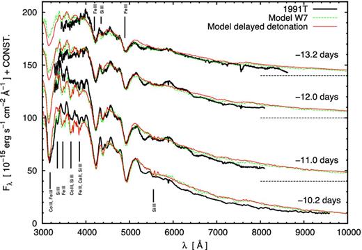
The early spectra of 1991T compared with the best-fitting models with a W7 and a delayed detonation density profile. The dashed lines on the right represent the zero values of the spectra.
Fe-Group elements. The most prominent features in these spectra are the deep Fe iii features at 4200 Å and 4900 Å. These lines get deeper with time as the photosphere recedes inside the ejecta. The models reproduce the strength and position of these features quite well. Ni, Co, and Fe need to be present to very high velocity (∼17 000 km s−1) for the model to reproduce the shape of the spectrum together with the U-band magnitudes. Fe-group elements are rich in near-UV lines, which redistribute the flux to redder wavelengths (Mazzali 2000). Moreover, 56Ni needs to be present in the outer layers of the ejecta in order to reproduce the deep absorption at 3200 Å observed in the spectrum at −10.2 d. This sharp feature is identified as a blend of Co iii and Fe iii lines, and Co can only be produced by 56Ni decay. The feature unfortunately is not observed in earlier spectra, which have a shorter wavelength coverage, and so it is not possible to constrain more accurately the 56Ni abundance at the highest velocities. Modelling a 91T-like SN Hatano et al. (2002) suggested that at high velocity there is no need for 56Ni because of the absence of Co iii lines. However, their models and observations do not study the region within 3100 and 3400Å where we indeed find strong evidence of Co iii lines.
Interestingly, some stable Fe is also needed in the outer layers in order to reproduce the deep Fe iii lines in the earliest spectrum, which dates about one week after the explosion. At such an early epoch 56Co did not have time to decay to 56Fe. The amount of Fe needed is consistent with solar metallicity. It most likely originates in the progenitor.
Calcium. Most SNe Ia show very strong Ca ii lines (H&K and IR triplet) throughout the early phase. SN 1991T is different. At the earliest epochs, the IR triplet is practically absent. Ca ii H&K lines contribute, together with Fe iii and Si iii, to a weak feature near 3800 Å. Ca ii lines strengthen only later. No Ca ii high-velocity features (HVFs) are observed in the early phases, unlike in most SNe Ia (Mazzali et al. 2005a), but this is primarily the effect of temperature. The behaviour of the HVF of Ca H&K and IR at later epochs (Section 3.3), when the feature appears, can be used to estimate the abundance of Ca between 13 000 and 17 000 km s−1. We set an upper limit on the abundance of Ca at the highest velocities that we can investigate where one can expect Ca from the progenitor to remain unburned. We derive X(Ca) < 0.0003 at v > 17 000 km s−1. This is comparable with the solar fraction of this element. Hence, the Ca in the outer shells most likely originates from the progenitor. The mass at high velocity (∼0.8 × 10⁻⁴ M⊙) is a tiny fraction of the total mass of Ca, which is more abundant at lower velocities. Hence, the uncertainties on the total mass of Ca arise from the abundance at lower velocities.
Silicon, sulphur, and magnesium. Among these IME, Si is the only element that is clearly identifiable in the early spectra. The ionization ratios of Si are very high compared with normal SNe Ia at similar epoch. The Si iii line near 4400 Å is easily identifiable in all the spectra. It is due to Si iii 4553 Å, 4568 Å, 4575 Å. Si iii 5740 is weak but still recognizable in this early epoch near 5600 Å. The line disappears from the model using a lower temperature. On the other hand, in models with an even higher temperature the Si iii 5740 line in the earliest spectrum becomes too strong and does not match the observations. The Si ii line at 6100 Å, which is the hallmark of SNe Ia, does not appear at these epochs and this behaviour is correctly reproduced.
S does not have any clear line at these epochs. Still, the abundance of the element can be constrained at velocities above 12 000 km s−1 using later spectra. Sulphur does not show up in the early spectra because it is highly ionized and there are no strong lines from these species in the observed wavelengths.
The only strong Mg line in SNe Ia is Mg ii 4481Å near 4200 Å, but in SN 1991T the ionization largely favours the double ionized species, which have no strong lines, and the feature is dominated by Fe. The amount of Mg is better constrained by the nebular model.
Carbon and oxygen. There are no clear C lines in the early spectra of SN 1991T. The upper limit for C abundance in the outer layers is X(C) = 0.005 and it comes from the appearance of C ii lines. The model cannot test the C abundance above 24 000 km s−1. These correspond to an upper limit of ∼0.01 M⊙ of C with the WDD3 density. An extensive discussion on the upper limits on the C abundance is presented in Section 5.1. Because of the high ionization, the O i line at 7500 Å appears only in much later spectra. O i has no strong lines in the optical. However, by exclusion we conclude that O is the dominant element in the outer layers.
Spectra before B-maximum
In Fig. 2 we compare the spectra from −9.0 d to −4.2 d since B-maximum with the best-fitting model. As in the previous series of spectra, SN 1991T shows deep lines from Fe-group elements and only weak lines from IMEs. Only in the last of these spectra Si ii 6355 begins to appear. The photospheric velocities of the model range between 11 500 and 10 200 km s−1.
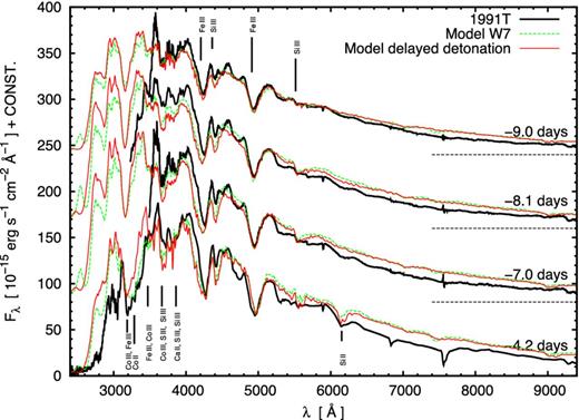
The spectra before maximum of 1991T compared with the best-fitting models with a W7 and a delayed detonation density profile. The spectrum at −4.2 d is connected with an UV spectrum observed from IUE at −2 d. The dashed lines on the right represent the zero values of the spectra.
The observed spectrum at −4.2 d is a merging of an optical spectrum and a UV spectrum obtained by the International Ultraviolet Explorer (IUE) observed 2 d before maximum. IUE obtained three good UV spectra of SN 1991T between −2 d and maximum and they show little variation. We connect the spectrum obtained at −2 d to the nearest available optical spectrum. The UV spectrum has been rescaled in order to match in the overlapping wavelength range with the optical spectrum.
Fe-Group elements. At the epochs covered in Fig. 2 the Fe iii features at 4200 Å and 4900 Å keep increasing in strength. The model reproduces this behaviour well. Much more 56Ni is required below 12 000 km s−1 than in the outer layers to block the UV flux. Moreover, Co ii is required to reproduce the absorption feature at 3200 Å. Also, some stable Fe is required to reproduce the strong Fe iii lines.
Calcium. The contribution of Ca to the absorption feature at 3800 Å remains weak. In normal SNe Ia the Ca ii H&K feature is dominant, but in SN 1991T it appears only at later epochs. Also at these lower velocities, there is no need for a large amount of Ca.
Silicon, sulphur, and magnesium. The ionization degree of these elements remains very high at these epochs compared with normal SNe Ia. Si ii 6355 Å appears clearly only at −4.2 d; instead the Si iii lines at 5500 Å and especially at 4450 Å are present at all epochs in this phase.
S iii contributes weakly to the absorption feature at 3800 Å, but the spectra after maximum constrain better the abundances of this element. At −4.2 d the S ii features at 5300 Å and 5450 Å appear for the first time. Although they are very weak, they are extremely useful in order to follow the shift of the ionization state of IMEs from doubly to singly ionized species. The model is able to reproduce the redder of the two lines.
Fe iii still dominates the feature at 4200 Å, hence it is difficult to determine the correct amount of Mg from Mg ii 4481.
Carbon and oxygen. At these velocities neither C nor O are necessary to complete the abundance distribution. At −4.2 d a weak O i 7774 Å line is produced by the model near 7500 Å, but it is not yet present in the observed spectrum. It appears only after maximum.
Shortly before maximum, the spectrum of SN 1991T begins to change, and lines of singly ionized species first appear. This transition gives strong constraints on the model. The epoch of the transition is influenced by the luminosity, i.e. the assumed value of the distance. For a higher luminosity the temperature increases, making the model worse. This is not completely reversed by tuning other parameters. Changing the time of explosion makes the earliest spectra worse, while a change in the photospheric velocity ruins the fit of the velocity of many lines.
The model has too much flux below 3000 Å. The mismatch of the model in the UV may be explained with a possible rapid change in the shape of the UV spectrum during the time between the two epochs. Many spectral features change rapidly in this phase. This makes a significant change in the UV part of the spectrum plausible. On the other hand, we do not have a way to properly flux calibrate the UV spectrum. A calibration problem could also reconcile our model with the observation. The metallicity of the outer layers can be used to adjust the UV early spectra (Lentz et al. 2000) but reverse fluorescence may dominate this effect (Mazzali 2000; Sauer et al. 2008) leaving largely unaffected the visible part of the spectra (Mazzali et al. 2014). We miss early enough UV spectra to accurately constrain the metallicity of the outer layers.
The spectra after maximum
Fig. 3 compares spectra from 5.8 to 13.8 d after B-maximum with the best-fitting models. After maximum the spectrum of SN 1991T appears similar to normal SNe Ia, with lines of Fe-group elements and of IMEs. The photospheric velocities of the model range between 9100 and 7200 km s−1. In this phase, the model overestimates the near-infrared flux because of the failure of the assumption of blackbody emission at the photosphere. In a luminous SN Ia like SN 1991T 56Ni is located at high velocities (Mazzali et al. 2007b) and significant deposition of energy occurs above the model photosphere even a few days after maximum. Although most line features can be reproduced by our photospheric-epoch model, the spectra are not nicely reproduced overall, especially the later one. Although the models frequently overestimate the red tail of the spectrum, leading to a larger bolometric flux than observed, we do not expect this to cause an overestimate of the ionization state of the matter or to have a systematic effect on the occupation numbers of the atomic levels as long as the flux in the part of the spectrum that is most strongly coupled with the matter (lower than ∼5000 Å) is correctly reproduced, as is the case in our models. Thus, below v ∼ 9000 km s−1, rather than optimize the abundances of the photospheric model, we used those derived from the nebular model, which is sensitive to these low velocities for the same reasons which make our photospheric model fail.
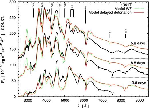
The spectra after maximum of 1991T with the best-fitting models. The spectrum at 5.8 d is plotted together with an UV spectrum observed by IUE at −0.4 d. The dashed lines on the right represent the zero values of the spectra.
The spectrum at 5.8 d after B-maximum is merged with the nearest available UV spectrum from the IUE. This was obtained at B-maximum, and rescaled in flux in order to match the part overlapping with the optical spectrum. The shape of the IUE spectrum does not change significantly over the two days from the previous spectrum, apart from a decrease in the flux.
Fe-group elements. In the nebular model at these velocities 56Ni and some stable Fe largely dominate the abundances. The Fe ii, Fe iii and Co ii lines are well reproduced. If a larger distance is used (meaning a more luminous supernova) at this epoch it is impossible to achieve the right ionization ratios. The ionization ratio that we mainly use as a proxy for temperature is the ratio of Fe iii and Fe ii lines, particularly the shape of the broad feature between 4700 and 5000 Å, which is a blend of an Fe ii-dominated absorption in the blue and Fe iii lines in the red. Moreover, in models with higher temperatures the strengthening of the Fe ii features near 4000 and 4200 Å after maximum occurs later. At these epochs, changing the time of explosion does not influence the spectrum significantly. Alternatively, increasing the velocity of the photosphere is not sufficient to decrease the temperature of the spectrum, but it would increase the velocity of the Fe lines, decreasing the quality of the fit.
Calcium. The Ca ii H&K lines near 3800 Å now become important, and they are reasonably reproduced by the model. Also the Ca ii IR lines are present in the spectra and are well reproduced by the model at the correct velocity, including some of the finer structure, neglecting the offset in flux. However, it is difficult to constrain strictly the abundance of Ca close to the velocity of the photosphere because its ionization favours the double ionized species and it strongly depends on little changes of other model parameters. The constraints on the Ca at high velocity are stronger because a larger fraction is singly ionized. At 5.8 d the high velocity component of Ca ii H&K shows as a dip on the blue side of the feature.
Sodium, silicon, sulphur. The deep feature at 5700 Å is most likely to be due to Na i D, but the code largely overestimates the ionization of sodium and cannot reproduce the line (Mazzali et al. 1997). At this epoch, S ii features appear clearly for the first time at 5300 Å and 5500 Å. The Si ii line at 6100 Å is also very important in the spectra. Si ii and S ii lines have a higher velocity than the photosphere because doubly ionized species are dominant at the photosphere. The line strength is difficult to reproduce using a larger distance because of the higher ionization ratios, but they are produced at the correct position and with the correct width (Fig. 3) with the best-fitting model. The red edge of the Si ii6355 Å line gets shallower with time. This effect is not due to Si but most likely to Fe ii lines. In particular, in the models at 13.8 d Fe ii6456 Å shows an absorption at ∼6240 Å. However, in our model the line is not as strong as in the observations.
Oxygen Although O is not present as these velocities, the broad feature at 7500 Å may be identified with O i 7774 Å. The model produces this line in the outer layers. The line in the models is not broad enough.
Summary of the photospheric analysis
We obtained good fits of a series of spectra covering a range of four weeks around B-maximum using abundance stratification. To fit the spectra we had to use a lower SN luminosity than most values in literature. Reddening and distance used in the best-fitting model are: E(B − V) = 0.12, μ = 30.57. The best rise time to B-maximum is 20.2 d. These values make SN 1991T somewhat less luminous than calculated in, e.g. Mazzali et al. (1995). The freedom in the rise time is limited to ±1 d thanks to the early spectra.
Compared with models with a higher luminosity there are major improvements in the ratio between the Si ii and Si iii features in the spectra after maximum (Fig. 3) and in the last spectrum of Fig. 2 (−4.2 d). A higher luminosity makes the features coming from doubly ionized species dominant. Also, it is possible to fit the Si ii feature in the spectra after maximum without producing too much Si iii absorption in the early spectra. Moreover, the O i feature in the spectra after maximum is reasonably reproduced, albeit with the wrong shape.
The uncertainties in the luminosity of the model and in the estimation of the extinction contribute to the uncertainty in the distance. On the other hand, the intrinsic luminosity of the model has much stronger constraints. Modelling SN 1991T allows us to have an estimate of the intrinsic luminosity of the object independently from the Phillips relation. The absolute B-magnitude at maximum obtained from the observed light curve (Richtler et al. 2001) and from the modelling is MB = −19.37.
An estimate of the uncertainty of this value could be ±0.15 mag. Due to the nature of the spectra the upper limit on the luminosity of the object is convincing.
An important improvement over Mazzali et al. (1995) is the good agreement with the UV flux at all epochs, including the earliest U photometry.
From the spectra in Figs 1–3 it appears that changing the density profile does not lead to significant changes in the synthetic spectra. Hence, trying different density profiles does not seem a good way to discriminate among different explosion models on 1991T-like SNe. However, their high luminosity seems to favour energetic delayed detonations.
NEBULAR MODEL
A late-time spectrum of SN 1991T obtained on 1992 February 5 with the ESO 3.6-m telescope (+ EFOSC1) (Cappellaro et al. 1991) was selected for modelling. This date corresponds to 282 d after B-maximum, which is ∼302 d after explosion. We modelled the spectrum using the NLTE code described in Section 2.2. This spectrum was already modelled by Mazzali et al. (2007b), but the assumptions of distance and reddening were slightly different in that work, although none of the most important results changes significantly. We restrict our nebular analysis to this phase to be free from light echo that becomes important at phases >2yr (Schmidt et al. 1994).
We adopt the stratified version of the code and test both explosion models used for the early-time analysis. Our approach, in the spirit of abundance tomography, is to use the density distribution as given by the original models but to modify the abundance of the various elements in order to optimize the match to the observations. The criteria we use in this process are primarily to fit the width and flux of the strongest emission lines ([Fe ii] and [Fe iii]).
We are able to obtain reasonably good fits for both density stratification models, with only small difference between them (Fig. 4). In the case of W7 we find a 56Ni mass of 0.78 M⊙. 56Ni is located between 2000 and 13 000 km s−1, and is dominant between 4000 and 12 000 km s−1. The large extension of the 56Ni zone explains the width of the nebular emission lines, which are among the broadest for any SNe Ia (Mazzali et al. 1998). The inner layers are dominated by stable 54Fe, whose mass we estimate to be 0.27 M⊙. This is necessary in order to match the flux and shape of the lines, as well as to reach a reasonable ionization degree. The total production of NSE material is ∼1.16 M⊙.
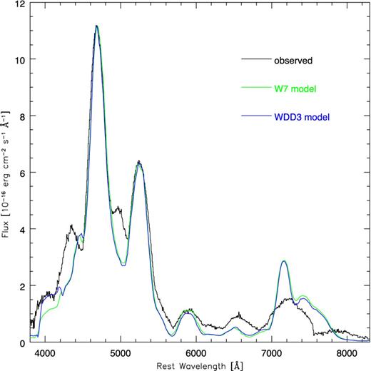
The nebular spectrum of SN 1991T obtained on 1992 Feb 5 (black) compared to two models, obtained using the W7 (green) and WDD3 (blue) densities.
The delayed detonation model yields the same 56Ni mass, 0.78 M⊙. The distribution with velocity is also similar. The DD model contains less mass in the lowest velocity shells, and this can be compensated by using less stable Fe in these zones, so the mass of 54Fe is now only 0.15 M⊙ and the total NSE mass is 0.94 M⊙. In both cases the mass of 58Ni is small (∼0.01 M⊙), as set by the non-detection of the line at 7378 Å.
The two fits are similar in quality, which makes it impossible to differentiate between these two models based on nebular spectroscopy. However, if we adopt the W7 density distribution, the abundances are not compatible with those of W7, while in the case of WDD3 they are closer to those of the original model (Iwamoto et al. 1999). This makes us favour the DD model.
ABUNDANCES OF ELEMENTS
Fig. 5 shows the abundances over radius in the best-fitting model with the delayed detonation density profile. Our model is compared with the original abundances. At velocities below 6000 km s−1 the abundances are from the nebular model. Between 6000 km s−1 and 9000 km s−1 the abundances from the nebular model are used in the photospheric models without changes; above 9000 km s−1 the abundances are from spectral models with the photospheric code.
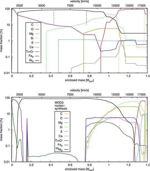
Abundances of the elements of the best-fitting model with the delayed detonation density profile of the SN 1991T (top panel, plotted in mass space). The abundances as a function of velocity are not significantly different between this model (obtained with the WDD3 density profile) and the one with the density profile of the W7 model (see text, and Fig. 7). The vertical dashed lines correspond to 6000 and 9000 km s−1. The abundances in this region are computed by the nebular model and used by the photospheric models without significant changes. The C abundance represented by the dotted line is the upper limit allowed in the model. The bottom panel represents the abundances of the WDD3 nucleosynthesis calculation. The major difference is the absence in our model of a Si dominated shell.
Our experience from computing many different models for the photospheric phase is that the stratification of abundances is quite fixed, but the whole picture can shift in velocity by about 1000 km s−1 depending on the rise time. This makes the measured masses of 56Ni (0.78 M⊙) and of O (0.29 M⊙) not very precise using the photospheric model alone. For example, reducing the rise time by half a day reduces the mass of O by 0.1 M⊙, increasing the mass of the Fe and 56Ni rich core while maintaining the photospheric spectra almost unchanged. On the other hand, the nebular model constrains precisely the mass of 56Ni (Section 4). The results of the nebular model are affected by the distance to the supernova. The uncertainties in this parameter will propagate to the estimate of the 56Ni mass. Hence, a safe estimate of the error over the Ni mass could be 0.05 M⊙.
The photospheric models need a significant amount of iron-group elements (∼4 per cent) at high velocity, above 12 000 km s−1. In particular about 3 per cent of 56Ni needs to be at high velocity to reproduce the broad and deep absorption feature comprising between 3200 Å and 3400 Å. The time evolution of the feature is well reproduced by the model. The main contributors to the feature are a large number of Co iii lines in the spectrum at −10.2 d, both Co iii and Co ii lines at −4.2 d and by Co ii lines afterwards. The Co ii lines contributing to the absorption feature have lower-lying levels, with energies mostly in the 2-3eV range. Removing 56Ni from the outer shells makes it impossible to reproduce the absorption feature, as is shown in Fig. 6 where the model with the delayed detonation density profile is shown with and without the high-velocity 56Ni. This is a refinement over the modelling from Mazzali et al. (1995), who claimed that SN 1991T was dominated by iron-group element also in the outer layers. That result came from requiring an excessively high luminosity because of the assumption of a larger distance than adopted here. We should stress again that the lower distance is preferred because it yields generally improved fits to the spectra at all photospheric epochs. Lowering the ionization actually increases the intensity of Fe iii lines in the spectra given the same abundances. This lower luminosity proved crucial to model many other characteristics of the spectra.
The presence of 56Ni in the outer layers has some of the characteristics of a HVF (Mazzali et al. 2005b). This 56Ni is placed at a velocity much higher than the majority of the elements. The high-velocity shell is devoid of C and made mostly by O. A similar behaviour is typically shown also by the Ca HVFs.
The abundances of other elements are also measured by the model with some accuracy. In Fig. 6 a model with 10 per cent of C in the outer shell is also shown. This is much more than what can be allowed to reproduce the spectra. At both epochs the ionization ratio favours the C ii species at high velocity. In the C-enriched model C ii features at 6370 Å and at 7000 Å are produced by lines with lower levels at 14 and 16eV, respectively. The occupation numbers of these levels drop in the spectra after maximum because of the lower temperature. Instead, the occupation levels are optimal to detect the line in pre-maximum spectra. On the other hand, the increasing temperature of the radiation field at early epochs (earlier than a week before maximum) favours species of C with a higher ionization also in the outer layers. It is possible to obtain a strict upper limit on the amount of C in the supernova using the spectra before maximum. C must be less than 0.5 per cent in the O-rich shell, because the C ii lines that appear already with this quantity of C are not present in any of the observed spectra.
The amount of Mg is quite uncertain, but it must be less than 20 per cent in the O-rich shell, because with this amount the line at 4300 Å becomes too deep owing to the contribution of Mg ii 4481 Å.
The amount of Si in the best-fitting model is about 0.14 M⊙. The uncertainty in this result can be estimated as 0.05 M⊙. This is large because the only really useful line is Si iii4450 Å. The Si ii6355 Å line in the post-maximum spectra is sensitive to the Si ii/Si iii ionization ratio, hence the actual luminosity of the model affects this line more than the abundance of Si itself. This is the same behaviour as the Si ii5972 Å line in normal SNe Ia (Hachinger et al. 2008). However, silicon, the most abundant IME, has a similar distribution in velocity also in models with larger luminosity. The shell where IMEs are most abundant is very narrow, between 10 000 km s−1 and 11 500 km s−1, and both 56Ni and O are present with significant abundances even in this shell. The narrow IME zone is the main difference between SN 1991T and other SNe Ia. The total amount of IMEs in the model is about 0.18 M⊙.
The abundance of Ca is determined from Ca ii H&K. At velocities lower than 13 000 km s−1, where the bulk of Ca is present, also this line is more sensitive to the ionization state than to the actual abundance of the element. The position of the line shows that this element must peak at a higher velocity than Si and S. The velocity range enriched in Ca is between 12 300 km s−1 and 12 500 km s−1. This is unexpected, because Ca is produced in explosive nucleosynthesis after Si and S, and the combustion progresses further to NSE going deeper into the star. Moreover, the ejecta show clear signs of 56Ni at even higher velocities. It looks like part of the ejecta underwent a more complete combustion in the outside and a progressively limited combustion in the inside. This is in contrast with the bulk of the ejecta, showing the usual stratification. This velocity ‘inversion’ between 56Ni, the Ca-rich layer, and the layer where the other IMEs are dominant, can be an important hint to understand the underlying explosion mechanism. This could be explained by ‘plumes’ of material with more complete burning expelled at velocities higher than the bulk of the ejecta. Another possible explanation could be the detonation of a thin He layer present in the outer part of the white dwarf. In the framework of the delayed detonation models, this layer may get triggered by the detonation front. The total amount of Ca found by the model is about 0.9 × 10⁻³ M⊙. On the other hand, it is known that high-velocity Ca ii lines exist in most SNe Ia, and these may be the result of the interaction of SN ejecta with H-rich circumstellar material (Gerardy et al. 2004; Mazzali et al. 2005a; Tanaka et al. 2008).
Fig. 7 shows the abundances for the best-fitting W7 density profile. The overall picture is similar to the results of the WDD3 density model. However, there are significant differences in the centre. With the W7 model we obtain a larger amount of stable Fe in the centre (Section 4). The luminosity constrains the mass of 56Ni to be similar in the two nebular models. The larger mass of Fe-group elements in W7 is compensated by a lower mass of Si and other IMEs at intermediate velocities. Unfortunately, the amount of IMEs is difficult to test using nebular analysis. Velocities lower than ∼10 000 km s−1 are also difficult to assess via photospheric analysis because, although the velocity of the photosphere drops below this value at maximum, the ionization state of Si and S close to the photosphere is too high to affect the spectra. For these reasons with the W7 density profile we obtain a similar composition as with the WDD3 density, apart from a larger amount of stable Fe (∼0.27 M⊙) and correspondingly, a lower amount of IMEs (∼0.04 M⊙).
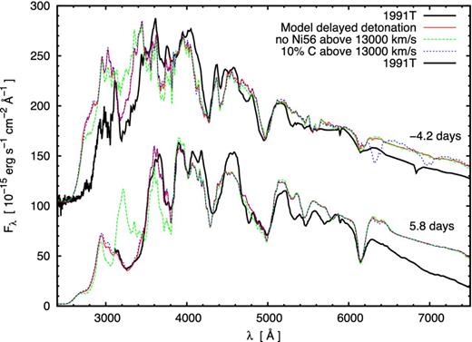
The spectra of 1991T at two significant epochs are compared with the delayed detonation density model. The effect of removing the high-velocity 56Ni or of adding a large quantity of C on the delayed detonation density model is shown to worsen the quality of the fit.
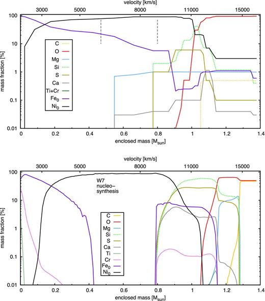
Abundances of the elements of the best-fitting model with the W7 density profile of the SN 1991T (top panel, plotted in mass space). The C abundance represented by the dotted line is the upper limit allowed in the model. The bottom panel represents the abundances of the W7 nucleosynthesis calculation. The major differences are the larger amount of 56Ni and stable Fe, the scarcity of IMEs and a large shell with O but no C. The major differences with the model based on the WDD3 density (Fig. 5) are more stable Fe, less IMEs and a stricter upper limit on C.
Carbon
Evaluating the amount of unburned material is very important to constrain different explosion models. We can estimate the amount of unburned material by measuring the abundance of C allowed in the model. This element must belong completely to the original composition of the CO white dwarf because, unlike O, it can only be destroyed by nuclear burning in an environment devoid of lighter elements.
There are no clear C lines in the spectra. In order to place an upper limit to the amount of this element in our model, we assume two different types of distribution for the element: a uniform abundance in the O-dominated shell, or all C being confined in an outer, unburned shell, which we assume to be composed of C and O in equal amounts.
The synthetic spectrum that is most affected by the uniform distribution of C in the O-rich shell is that at −4.2 d, because of the lower ionization which allows a C ii line at 6300 Å to appear. In Fig. 8 we compare two models, with and without C. Both models are based on the delayed detonation density profile. We set an upper limit of 0.5 per cent to the C abundance, because for lower values it is no longer possible to distinguish the C line; moreover the spectrum resolution is not accurate enough to sustain a tighter lower limit.
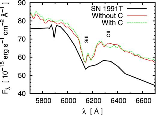
In the figure we compare the model with the amount of C in its upper limit with the model without this element. Only the section of the spectrum at −4.2 d affected by a small amount of C is shown.
The spectrum that is most influenced by introducing C at high velocity is the earliest one. Since SN 1991T was observed from quite early on and the first spectrum shows no clear evidence of C, the lower limit for the velocity of a shell of unburned material is quite high, that is 24 000 km s−1. The recently discovered, spectroscopically normal SN 2013dy shows strong C ii lines detached from the photosphere in the early epochs (Zheng et al. 2013). The velocity of these HVFs of C evolves to a minimum of ∼23 000 km s−1. Our model shows that if C is present in the peculiar SN 1991T it has to be at an even higher velocity.
Doubly ionized C is not useful in determining the upper limit of the C abundance. C iii lines appear in the spectra only with abundances high enough to produce strong C ii lines.
Combining the two upper limits, the model allows a maximum amount of C of 0.01 M⊙, at the expense of O, using the delayed detonation density profile.
With the W7 density, the upper limit to the amount of C is much lower (0.001 M⊙). The main reason is the much lower amount of material at high velocity, above ∼ 22 000 km s−1 in the W7 model. The C in this high-velocity material does not show up in the spectra with either the W7 or the delayed detonation density profile also with a 100 per cent abundance. With the W7 density the amount of C that can remain ‘hidden’ at such high velocities is negligible.
However, it is difficult to believe that there is no mixing of material at all at these very high velocities and that the interface between O and unburned material is so sharp. If there was some mixing or a smooth transition between these two zones, the maximum C mass allowed would be even lower. This is because a significant amount of C between 15 000 and 24 000 km s−1 would be easily detectable. At the same time, to have a smooth transition the amount of C above 24 000 km s−1 has to decrease significantly.
BOLOMETRIC LIGHT CURVE
To check the consistency of the model we compare the bolometric light curve with the observed magnitudes. We have calculated a bolometric light curve from the UBVRI photometry. For each epoch of observation (see Table A1 in Appendix A1, data from Altavilla et al. 2004; Lira et al. 1998), we constructed a spectral flux distribution using the flux zero-points of Fukugita, Shimasaku & Ichikawa (1995). For epochs when observations are missing in one or more filters, we interpolated the magnitudes using splines of the light curves. Since the light curves are well sampled and regular, this introduces a negligible uncertainty. The spectral flux distributions were dereddened with the extinction curve of Cardelli, Clayton & Mathis (1989), using E(B − V) = 0.12, splined and integrated in the wavelength range 3000–10 000 Å (a linear extrapolation of the flux was used bluewards of the limit of the U-band filter and redwards of the limit of the I-band filter). Using the distance modulus μ = 30.57 we derived bolometric luminosities, which are shown in Fig. 9. The near-infrared contribution to the observed bolometric light curve is difficult to estimate, because observations are only available at four epochs (Krisciunas et al. 2004). Using the observations, the near-infrared luminosities at these four epochs are estimated to be 14 per cent, 3.3 per cent, 3.5 per cent, and 6.4 per cent of the total luminosities in the optical and near-infrared. These contributions are small, and comparable to the uncertainty in the derived bolometric luminosity.
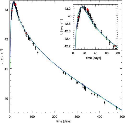
Synthetic bolometric light curves based on the results obtained using the density structures and the abundance distributions derived for W7 (green) and WDD3 (blue) compared to the UBVRI pseudo-bolometric light curve of SN 1991T (black points). The correction for the infrared flux is shown as red points for the few epochs in which it was possible to derive it based on the published data.
We produced synthetic bolometric light curves using the code described in Section 2 and the abundances derived from spectral modelling. In the spirit of abundance tomography, this is a test that the derived abundance (and density) distribution is appropriate for the SN at hand. We used both the W7 and WDD3 densities and the abundance stratification derived from the respective tomography experiments. The results are shown in Fig. 9 and compared to the light curve of SN 1991T. From the synthetic spectra we can set an upper limit of 10 per cent for the NIR contribution to the total spectral flux at all epochs where spectra were computed. Based on these considerations, we can safely neglect the NIR contribution to the bolometric luminosity. The agreement is satisfactory in both cases. Bolometric maximum is reached about 18 d after explosion with both models. The differences between the two model light curves are smaller than the uncertainties in the construction of the bolometric light curve and those deriving from the use of a constant opacity in the model. At later times, the two light curves are basically indistinguishable, because the two models have the same 56Ni mass.
CONSISTENCY OF THE MODEL
The amount of 56Ni in our best-fitting model with the delayed detonation density profile for SN 1991T is ∼0.78 M⊙. Stable Fe is about 0.15 M⊙, there are some IMEs (only ∼0.18 M⊙), the rest is supposed to be O (0.29 M⊙) while essentially no C is present.
In the model with the W7 density profile the amount of stable Fe is larger, ∼0.27. The quantity of 56Ni is similar, ∼0.78 M⊙. The 56Ni mass correlates strongly with the luminosity in the nebular phase. The mass of the IMEs is smaller (only ∼0.04 M⊙) and the amount of O is similar (∼0.30 M⊙).
The maximum absolute bolometric luminosity computed from the photometry with the distance modulus and reddening used here is 1.7 × 1043erg s−1. Using this luminosity together with a version of the Arnett's rule (Arnett 1982) from Stritzinger et al. (2006) we derive for SN 1991T ∼0.85 M⊙ of 56Ni, with an error of about ±15 per cent. This is consistent with the value we derived (0.78 M⊙).
Nucleosynthesis.
| W7 density | WDD3 density | |
|---|---|---|
| O | 0.30 M⊙ | 0.29 M⊙ |
| IME | 0.04 M⊙ | 0.18 M⊙ |
| 56Ni | 0.78 M⊙ | 0.78 M⊙ |
| stable Fe | 0.27 M⊙ | 0.15 M⊙ |
| |$E_K^{{\rm from nucl.}}$| | 1.27 × 1051erg | 1.24 × 1051erg |
| EK | 1.30 × 1051 erg | 1.43 × 1051 erg |
| W7 density | WDD3 density | |
|---|---|---|
| O | 0.30 M⊙ | 0.29 M⊙ |
| IME | 0.04 M⊙ | 0.18 M⊙ |
| 56Ni | 0.78 M⊙ | 0.78 M⊙ |
| stable Fe | 0.27 M⊙ | 0.15 M⊙ |
| |$E_K^{{\rm from nucl.}}$| | 1.27 × 1051erg | 1.24 × 1051erg |
| EK | 1.30 × 1051 erg | 1.43 × 1051 erg |
We find that it is possible to achieve good fits only with a lower luminosity than what some of the distance estimates imply. Measures of distance to the host galaxy of SN 1991T are quite different (Table 1), and the distance modulus used here is compatible with most of these measurements. Moreover, it is difficult to distinguish our model from one with a distance modulus increased by 0.1 mag and reddening decreased by 0.03 mag, because these two parameters have a similar effect on the spectra. The uncertainty on the extinction is larger than that on the distance.
In this work we used the density profiles as given. Among all elements used to fit the spectra, O has the smallest direct effects on the spectra. Relaxing the constraint on the density profile can improve the energetic consistence of the fit. It is possible to remove some of the oxygen while still preserving good spectral fits in the early epochs. This means removing up to ∼0.1 M⊙ of O from the external layer. However, although O in the outer layers does not produce strong lines (with the exception of the O i line at 7500 Å), its presence increases the electron density. This is important for the ionization balance of the other elements. Removing O increases the ionization, and a smaller amount of Fe is needed above ∼16 000 km s−1than with the W7 or the WDD3 densities. Differently from what happens with these density profiles, the Fe from 56Co decay is enough to reproduce the Fe iii lines in the pre-maximum epochs.
The presence of less material at high velocity is also suggested by the kinetic energy balance. The density profiles used here have too much kinetic energy compared to the nucleosynthesis. The kinetic energy can be significantly reduced by modifying the outer layers. It is important to keep in mind that the balance of the kinetic energy assumes a Chandrasekhar mass white dwarf. This discussion does not necessarily mean that we suggest a mass lower than 1.4 M⊙. Most likely, the mass subtracted from the outer layers can be redistributed in the much more massive inner parts without too much changes in the spectra. A low-density layer at high velocities, composed of 56Ni and Ca, could be an important clue of the explosion mechanism.
On the other hand, a low density at high velocity with a significantly lower kinetic energy could be an indication of a Super-Chandrasekhar mass ejecta. This would also naturally explain the abundance of stable iron in the centre inferred from nebular spectroscopy. The slow evolution of the light curve is also favoured by a larger total mass. In any case the deviation from the Chandrasekhar mass should not exceed 10 per cent.
Changing the density profile of the ejecta to explore these possibilities should be done using some supporting models that assure hydrodynamic consistency. Otherwise there may be too many free parameters to be investigated and there is the risk to end up with an unphysical density profile. This scenario deserves careful investigation, but this exceeds the aim of this work.
COMPARISON WITH EXPLOSION MODELS
The distribution of elements rules out strong mixing as predicted by three-dimensional deflagration models (e.g. Gamezo, Khokhlov & Oran 2005; Röpke & Hillebrandt 2005; Röpke et al. 2007). Delayed detonation models are much more consistent with the distribution of the elements inferred by modelling the spectra (see e.g. Gamezo et al. 2005). However, the distribution of IMEs that results from the model of 1991T is different from that produced by delayed detonation models. In SN 1991T there is only a small Si-dominated shell located between the interior dominated by 56Ni and the external O-dominated shell (Fig. 5).
A delayed detonation model with more complete burning leads to more 56Ni at the expense of O and C, also decreasing the mass of Si. For example, model DD_005 from Röpke & Niemeyer (2007) shows a reasonable agreement in the total mass of the principal elements. But looking more carefully there are still some minor problems comparing it with the abundances of our model of SN 1991T (Fig. 5). In their model the C mass is consistent with the upper limits from our models, but the O mass is too low and the IMEs mass is still too high. The behaviour of this model, where an almost complete burning of C implies also a large depletion of O and a large production of IMEs, is a common behaviour of strong delayed detonation models. This does not make it easy to explain the large amount of O that we found in SN 1991T together with the low mass of IMEs and C in the framework of delayed detonation models. In the model TURB7 of Bravo et al. (2009) the elemental abundances are very similar to those of DD_005. Although the final abundances are not too different from our results, the distribution of elements in TURB7 is very different. In the TURB7 model there is an excess of Fe-group elements in the outer layers. The IMEs reach a maximum in the outer layers, while in our models the maximum is reached at intermediate velocities, both in the delayed detonation model and in W7. The O abundance has a maximum in an intermediate shell at an enclosed mass of 1 M⊙, while in our model of SN 1991T there is no more O at that depth. The distribution of elements of SN 1991T matches well the distribution of the TURB7 model just at the end of the detonation before most of the mixing when the ejecta are not yet in homologous expansion. The inversion of the IMEs- and the O-rich layers in TURB7 takes place because the former has a higher velocity than the latter. According to Bravo et al. (2009) the mixing that changes the abundances after the end of the detonation happens in any model with a detonation that propagates inwards from a point close to the surface. Indeed, the delayed detonation model ‘case c’ from Gamezo et al. (2005), which has a central detonation ignition, has much more stratified ejecta. The model has also the right velocity of the Si-rich shell. However, the explosion model ‘case c’ has too much Si and too much unburned C. Moreover, 56Ni does not reach the outer layers as it does in SN 1991T. A slightly off-centre ignition may accomplish some more mixing, so some Fe group elements could end up in the outer parts of the ejecta, while keeping a well-defined Si-rich shell. The 3D delayed detonation models from Seitenzahl et al. (2013) have a stratification of the outer part of the ejecta in fair agreement with what is inferred from our model of SN 1991T. In particular, the models with few ignition spots show a larger production of 56Ni at the expenses of IMEs. The inner parts, however, show significant mixing of stable Fe with 56Ni. This is claimed to be a 3D effect of the deflagration phase that does not appear in 2D models. However, this does not agree with the results of the nebular spectra analysis of our model of SN 1991T (and other SNe Ia) where stable Fe is concentrated in the centre. In conclusion, strong delayed detonation models are good candidates for roughly explaining the distribution of the elements inferred from our model of SN 1991T, but the finer details are hard to explain with the current explosion models.
CONCLUSIONS
SN 1991T was a peculiar, overluminous supernova, well observed from early phases. It can be considered a good representative of a class of extreme SNe Ia. Although SN 1991T is extreme among nearby SNe Ia, we expect supernovae of this subclass to be common at cosmological distances, because they are selected by the Malmquist bias.
We obtained the abundance distribution of SN 1991T modelling the optical spectra in the photospheric and the nebular phase. The distribution of elements in SN 1991T consists of an inner layer rich of stable Fe, a large intermediate layer composed mainly of 56Ni and an outer zone rich of O. IMEs are dominant only in a narrow shell at the interface between the 56Ni-rich and O-rich zones.
Shortage of IMEs is a major peculiarity of SN 1991T that arises from our analysis. Comparing the resulting abundance profile with explosion models from the literature suggests that deflagration models do not produce enough burning and mix up the elements too much. We checked the consistency of the bolometric light curve and of the kinetic energy of the assumed density profile of the ejecta.
Delayed detonation models are better suited for the SN 1991T. To produce enough 56Ni a delayed detonation model needs an early transition to a detonation. However, such models may burn O to IMEs too efficiently and at the same time leave too much unburned C in external layers.
We see no need for a mass exceeding the Chandrasekhar limit from a combined photospheric and nebular approach. The modelling allows us to set a convincing upper limit on the luminosity of the object. Our best model has a luminosity of MB = −19.37.
A differential study of SN 1991T and other similarly luminous but spectroscopically normal SNe Ia (e.g. SN 1999ee) may shed more light on the differences between them and the fine details of these extreme explosions.
This work has made use of the SUSPECT SN spectral archive. This work has made use of the WISeREP data repository. For the UV spectra we make use of the MAST archive.
We thank the Mongolian Ger Camps for the hospitality while this work was finished in the Gobi desert.
PM, EC, and SB are partially supported by the PRIN-INAF 2011 with the project ‘Transient Universe: from ESO Large to PESSTO’.
KN acknowledges the support from the Grant-in-Aid for Scientific Research (23224004, 23540262, 26400222) from the Japan Society for the Promotion of Science, and the World Premier International Research Center Initiative (WPI Initiative), MEXT, Japan.
Hamamatsu Professor.
REFERENCES
APPENDIX A: MAGNITUDES
Reports the magnitudes used for the calculation of the bolometric light curve. The codes for the source column are as follow: 0,1 = Altavilla et al. (2004), 2 = Lira et al. (1998), 3 = Schmidt et al. (1994) and the IAUCs Gilmore (1991), Barlow et al. (1991), Wheeler, Smith & Gilmore (1991), Bateson et al. (1991), Holberg et al. (1991), Menzies et al. (1991).
| JD + 240 0000 | U | B | V | R | I | Source |
|---|---|---|---|---|---|---|
| 48362.85 | 12.26 ± .02 | 12.98 ± .02 | 12.84 ± .02 | 12.67 ± .02 | 12.87 ± .02 | 1 |
| 48363.65 | ⋅⋅⋅ | 12.73 ± .01 | 12.61 ± .01 | ⋅⋅⋅ | ⋅⋅⋅ | 1 |
| 48363.77 | ⋅⋅⋅ | 12.712 ± .016 | 12.618 ± .016 | 12.526 ± .015 | ⋅⋅⋅ | 2 |
| 48363.80 | 12.04 ± .02 | 12.80 ± .02 | 12.74 ± .02 | ⋅⋅⋅ | ⋅⋅⋅ | 1 |
| 48364.46 | 11.80 ± n/a | 12.51 ± n/a | 12.40 ± n/a | ⋅⋅⋅ | ⋅⋅⋅ | IAUC5246 |
| 48364.64 | ⋅⋅⋅ | 12.46 ± .01 | 12.34 ± .01 | 12.32 ± .01 | ⋅⋅⋅ | 1 |
| 48364.76 | ⋅⋅⋅ | 12.449 ± .016 | 12.362 ± .016 | 12.299 ± .015 | ⋅⋅⋅ | 2 |
| 48365.65 | ⋅⋅⋅ | ⋅⋅⋅ | ⋅⋅⋅ | 12.159 ± .015 | ⋅⋅⋅ | 2 |
| 48365.66 | 11.610 ± .026 | 12.362 ± .016 | 12.256 ± .016 | 12.134 ± .015 | 12.215 ± .017 | 2 |
| 48366.67 | ⋅⋅⋅ | 12.06 ± .01 | 12.00 ± .01 | 11.97 ± .01 | ⋅⋅⋅ | 1 |
| 48366.67 | ⋅⋅⋅ | 12.152 ± .016 | 12.061 ± .016 | 11.971 ± .015 | ⋅⋅⋅ | 2 |
| 48367.65 | ⋅⋅⋅ | ⋅⋅⋅ | 11.89 ± .01 | ⋅⋅⋅ | ⋅⋅⋅ | 1 |
| 48367.77 | 11.09 ± n/a | 11.75 ± n/a | 11.69 ± n/a | ⋅⋅⋅ | ⋅⋅⋅ | IAUC5270 |
| 48367.77 | 11.09 ± n/a | 11.76 ± n/a | 11.70 ± n/a | ⋅⋅⋅ | ⋅⋅⋅ | IAUC5270 |
| 48368.02 | 11.14 ± n/a | 11.94 ± n/a | 11.84 ± n/a | 11.76 ± n/a | ⋅⋅⋅ | IAUC5246 |
| 48368.70 | ⋅⋅⋅ | 11.78 ± .01 | 11.80 ± .01 | 11.70 ± .01 | ⋅⋅⋅ | 1 |
| 48372.70 | ⋅⋅⋅ | 11.748 ± .016 | ⋅⋅⋅ | 11.533 ± .015 | 11.693 ± .017 | 2 |
| 48374.64 | 11.282 ± .026 | 11.719 ± .016 | 11.573 ± .016 | 11.511 ± .015 | 11.690 ± .017 | 2 |
| 48374.64 | 11.304 ± .026 | 11.707 ± .016 | 11.560 ± .016 | 11.519 ± .015 | 11.694 ± .017 | 2 |
| 48375.01 | 11.01 ± n/a | 11.66 ± n/a | 11.52 ± n/a | 11.41 ± n/a | ⋅⋅⋅ | IAUC5253 |
| 48375.65 | 11.270 ± .026 | 11.720 ± .016 | 11.537 ± .016 | 11.509 ± .015 | 11.676 ± .017 | 2 |
| 48375.65 | 11.370 ± .026 | 11.715 ± .016 | 11.568 ± .016 | 11.529 ± .015 | 11.689 ± .017 | 2 |
| 48376.69 | 11.233 ± .026 | 11.741 ± .016 | 11.527 ± .016 | 11.475 ± .015 | ⋅⋅⋅ | 2 |
| 48376.69 | 11.279 ± .026 | 11.696 ± .016 | 11.542 ± .016 | 11.474 ± .015 | ⋅⋅⋅ | 2 |
| 48376.69 | ⋅⋅⋅ | ⋅⋅⋅ | ⋅⋅⋅ | ⋅⋅⋅ | 11.690 ± .017 | 2 |
| 48376.97 | 11.21 ± n/a | 11.75 ± n/a | 11.49 ± n/a | 11.36 ± n/a | 11.69 ± n/a | IAUC5256 |
| 48377.62 | 11.329 ± .026 | 11.694 ± .016 | 11.511 ± .016 | 11.435 ± .015 | 11.664 ± .017 | 2 |
| 48377.62 | ⋅⋅⋅ | 11.711 ± .016 | 11.482 ± .016 | 11.435 ± .015 | 11.665 ± .017 | 2 |
| 48380.69 | ⋅⋅⋅ | ⋅⋅⋅ | 11.529 ± .016 | 11.479 ± .015 | 11.805 ± .018 | 2 |
| 48380.70 | ⋅⋅⋅ | 11.832 ± .016 | 11.525 ± .016 | 11.466 ± .015 | 11.788 ± .017 | 2 |
| 48381.60 | ⋅⋅⋅ | 11.836 ± .016 | 11.535 ± .016 | 11.518 ± .015 | 11.847 ± .017 | 2 |
| 48381.60 | ⋅⋅⋅ | 11.857 ± .016 | ⋅⋅⋅ | 11.501 ± .015 | 11.846 ± .017 | 2 |
| 48382.67 | ⋅⋅⋅ | 11.912 ± .016 | 11.577 ± .016 | 11.565 ± .015 | 11.915 ± .017 | 2 |
| 48382.68 | ⋅⋅⋅ | 11.919 ± .016 | 11.575 ± .016 | 11.552 ± .015 | 11.917 ± .017 | 2 |
| 48382.77 | 11.78 ± n/a | 11.98 ± n/a | 11.61 ± n/a | ⋅⋅⋅ | ⋅⋅⋅ | IAUC5273 |
| 48383.58 | 11.652 ± .026 | 11.959 ± .016 | 11.605 ± .016 | 11.589 ± .015 | 11.966 ± .017 | 2 |
| 48383.58 | ⋅⋅⋅ | 11.971 ± .016 | 11.583 ± .016 | 11.585 ± .015 | 11.967 ± .017 | 2 |
| 48385.62 | ⋅⋅⋅ | ⋅⋅⋅ | ⋅⋅⋅ | 11.729 ± .015 | 12.049 ± .017 | 2 |
| 48385.63 | ⋅⋅⋅ | 12.137 ± .016 | 11.643 ± .016 | 11.730 ± .015 | 12.051 ± .017 | 2 |
| 48386.55 | ⋅⋅⋅ | 12.208 ± .016 | ⋅⋅⋅ | ⋅⋅⋅ | ⋅⋅⋅ | 2 |
| 48386.55 | ⋅⋅⋅ | 12.248 ± .016 | 11.764 ± .016 | 11.811 ± .015 | 12.087 ± .017 | 2 |
| 48388.57 | 12.381 ± .026 | 12.408 ± .016 | 11.873 ± .016 | 11.917 ± .015 | ⋅⋅⋅ | 2 |
| 48390.50 | 12.750 ± .026 | 12.603 ± .016 | 11.974 ± .016 | 11.982 ± .015 | 12.076 ± .017 | 2 |
| 48390.50 | 12.778 ± .026 | 12.600 ± .016 | 11.971 ± .016 | 11.976 ± .015 | 12.062 ± .017 | 2 |
| 48393.62 | 13.222 ± .026 | 12.965 ± .016 | 12.150 ± .016 | 12.029 ± .015 | 12.022 ± .017 | 2 |
| 48395.55 | ⋅⋅⋅ | 13.131 ± .016 | 12.223 ± .016 | ⋅⋅⋅ | ⋅⋅⋅ | 2 |
| 48395.56 | ⋅⋅⋅ | 13.149 ± .016 | 12.247 ± .016 | ⋅⋅⋅ | ⋅⋅⋅ | 2 |
| 48396.56 | ⋅⋅⋅ | 13.39 ± .01 | 12.32 ± .01 | 12.32 ± .01 | ⋅⋅⋅ | 1 |
| 48396.56 | ⋅⋅⋅ | 13.48 ± .01 | 12.29 ± .01 | ⋅⋅⋅ | ⋅⋅⋅ | 1 |
| 48396.56 | ⋅⋅⋅ | ⋅⋅⋅ | 12.45 ± .01 | ⋅⋅⋅ | ⋅⋅⋅ | 1 |
| 48405.59 | ⋅⋅⋅ | 14.071 ± .016 | 12.731 ± .016 | 12.378 ± .015 | 12.098 ± .017 | 2 |
| 48405.59 | ⋅⋅⋅ | 14.071 ± .017 | 12.735 ± .016 | 12.379 ± .015 | 12.111 ± .017 | 2 |
| 48414.62 | 14.610 ± .026 | 14.302 ± .016 | 13.123 ± .016 | 12.820 ± .015 | 12.421 ± .017 | 2 |
| 48414.62 | ⋅⋅⋅ | 14.307 ± .016 | ⋅⋅⋅ | ⋅⋅⋅ | ⋅⋅⋅ | 2 |
| 48420.47 | 14.862 ± .026 | 14.556 ± .016 | 13.423 ± .016 | 13.102 ± .015 | 12.819 ± .017 | 2 |
| 48427.67 | ⋅⋅⋅ | 14.77 ± .01 | 13.60 ± .01 | 13.51 ± .01 | ⋅⋅⋅ | 1 |
| 48427.67 | ⋅⋅⋅ | ⋅⋅⋅ | 13.59 ± .01 | ⋅⋅⋅ | ⋅⋅⋅ | 1 |
| 48427.67 | ⋅⋅⋅ | ⋅⋅⋅ | 13.66 ± .01 | 13.45 ± .01 | ⋅⋅⋅ | 1 |
| 48431.49 | 15.032 ± .030 | 14.770 ± .017 | 13.744 ± .016 | 13.527 ± .015 | 13.386 ± .017 | 2 |
| 48431.49 | 15.070 ± .030 | 14.746 ± .017 | 13.754 ± .016 | ⋅⋅⋅ | ⋅⋅⋅ | 2 |
| 48438.50 | ⋅⋅⋅ | 14.863 ± .016 | 13.936 ± .016 | ⋅⋅⋅ | 13.712 ± .017 | 2 |
| 48439.47 | ⋅⋅⋅ | 14.919 ± .016 | 14.018 ± .016 | 13.824 ± .015 | 13.749 ± .017 | 2 |
| 48439.47 | ⋅⋅⋅ | 14.931 ± .016 | 13.986 ± .016 | 13.830 ± .015 | 13.738 ± .017 | 2 |
| 48439.83 | ⋅⋅⋅ | 14.91 ± n/a | 14.03 ± n/a | ⋅⋅⋅ | ⋅⋅⋅ | IAUC5309 |
| 48440.46 | ⋅⋅⋅ | 14.897 ± .016 | 14.059 ± .016 | 13.859 ± .001 | 13.821 ± .017 | 2 |
| 48440.46 | ⋅⋅⋅ | 14.917 ± .016 | 14.058 ± .016 | 13.872 ± .015 | 13.790 ± .017 | 2 |
| 48440.87 | ⋅⋅⋅ | 14.92 ± n/a | 14.00 ± n/a | ⋅⋅⋅ | ⋅⋅⋅ | IAUC5309 |
| 48442.48 | 15.265 ± .026 | 14.888 ± .016 | 14.045 ± .016 | 13.888 ± .015 | 13.778 ± .017 | 2 |
| 48445.46 | ⋅⋅⋅ | ⋅⋅⋅ | 14.139 ± .016 | ⋅⋅⋅ | ⋅⋅⋅ | 2 |
| 48445.47 | ⋅⋅⋅ | 14.934 ± .017 | 14.143 ± .016 | ⋅⋅⋅ | ⋅⋅⋅ | 2 |
| 48459.49 | ⋅⋅⋅ | 15.115 ± .016 | 14.476 ± .016 | 14.407 ± .015 | 14.538 ± .017 | 2 |
| 48469.51 | ⋅⋅⋅ | 15.42 ± .02 | ⋅⋅⋅ | 14.78 ± .02 | ⋅⋅⋅ | 1 |
| 48480.49 | ⋅⋅⋅ | ⋅⋅⋅ | 15.29 ± .02 | ⋅⋅⋅ | ⋅⋅⋅ | 1 |
| 48593.46 | ⋅⋅⋅ | 16.95 ± .06 | 17.01 ± .05 | 17.59 ± .06 | ⋅⋅⋅ | 0 |
| 48593.46 | ⋅⋅⋅ | 16.98 ± .06 | 17.01 ± .05 | 17.62 ± .06 | ⋅⋅⋅ | 0 |
| 48594.46 | ⋅⋅⋅ | 17.06 ± .06 | 17.10 ± .06 | 17.65 ± .06 | ⋅⋅⋅ | 0 |
| 48597.8 | ⋅⋅⋅ | 17.20 ± .03 | 17.13 ± .03 | 17.65 ± .05 | 17.34 ± .08 | 3 |
| 48603.46 | ⋅⋅⋅ | 17.04 ± .06 | 17.07 ± .06 | 17.68 ± .06 | ⋅⋅⋅ | 0 |
| 48628.83 | ⋅⋅⋅ | 17.496 ± .019 | 17.484 ± .018 | ⋅⋅⋅ | 17.939 ± .040 | 2 |
| 48629.83 | ⋅⋅⋅ | 17.513 ± .018 | 17.475 ± .018 | ⋅⋅⋅ | 17.951 ± .046 | 2 |
| 48653.90 | ⋅⋅⋅ | 17.66 ± .05 | 17.95 ± .05 | 18.54 ± .05 | ⋅⋅⋅ | 1 |
| 48657.60 | ⋅⋅⋅ | ⋅⋅⋅ | 17.88 ± .07 | ⋅⋅⋅ | ⋅⋅⋅ | 0 |
| 48657.82 | ⋅⋅⋅ | 17.74 ± .04 | 17.96 ± .03 | 18.56 ± .04 | ⋅⋅⋅ | 1 |
| 48658.66 | ⋅⋅⋅ | 17.75 ± .04 | 17.94 ± .08 | 18.52 ± .06 | ⋅⋅⋅ | 0 |
| 48677.78 | ⋅⋅⋅ | ⋅⋅⋅ | 18.116 ± .022 | ⋅⋅⋅ | 18.367 ± .045 | 2 |
| 48681.78 | ⋅⋅⋅ | 18.02 ± .06 | 18.34 ± .05 | 18.97 ± .05 | ⋅⋅⋅ | 1 |
| 48686.46 | ⋅⋅⋅ | 18.25 ± .10 | 18.27 ± .06 | 19.00 ± .08 | ⋅⋅⋅ | 0 |
| 48687.85 | ⋅⋅⋅ | ⋅⋅⋅ | 18.343 ± .017 | 19.086 ± .022 | 18.489 ± .026 | 2 |
| 48688.46 | ⋅⋅⋅ | 18.25 ± .10 | 18.35 ± .06 | 19.05 ± .08 | ⋅⋅⋅ | 0 |
| 48688.8 | ⋅⋅⋅ | ⋅⋅⋅ | 18.35 ± .03 | 19.05 ± .05 | 18.43 ± .05 | 3 |
| 48691.78 | ⋅⋅⋅ | 18.445 ± .018 | 18.357 ± .019 | 19.080 ± .025 | 18.489 ± .031 | 2 |
| 48692.67 | ⋅⋅⋅ | 18.42 ± .07 | 18.42 ± .07 | 19.07 ± .06 | ⋅⋅⋅ | 1 |
| 48720.77 | ⋅⋅⋅ | 18.834 ± .023 | 18.765 ± .022 | ⋅⋅⋅ | 18.952 ± .034 | 2 |
| 48731.62 | ⋅⋅⋅ | ⋅⋅⋅ | 19.010 ± .052 | ⋅⋅⋅ | ⋅⋅⋅ | 2 |
| 48731.63 | ⋅⋅⋅ | 18.916 ± .078 | 18.947 ± .047 | ⋅⋅⋅ | ⋅⋅⋅ | 2 |
| 48742.8 | ⋅⋅⋅ | 19.00 ± .03 | 19.05 ± .03 | 19.64 ± .08 | 18.81 ± .09 | 3 |
| 48746.69 | ⋅⋅⋅ | 18.99 ± .05 | 19.12 ± .05 | 19.58 ± .05 | 19.00 ± .08 | 1 |
| 48776.53 | 20.346 ± .250 | 19.654 ± .078 | 19.662 ± .057 | 20.271 ± .102 | 19.374 ± .119 | 2 |
| 48776.54 | ⋅⋅⋅ | 19.773 ± .097 | 19.684 ± .063 | 20.162 ± .097 | 19.359 ± .113 | 2 |
| 48776.8 | ⋅⋅⋅ | 19.43 ± .03 | 19.49 ± .03 | 20.03 ± .08 | 19.08 ± .12 | 3 |
| 48829.67 | ⋅⋅⋅ | 19.97 ± .10 | 20.27 ± .05 | 20.57 ± .05 | ⋅⋅⋅ | 1 |
SUPPORTING INFORMATION
Additional Supporting Information may be found in the online version of this article:
Appendix Table A1:
Please note: Oxford University Press are not responsible for the content or functionality of any supporting materials supplied by the authors. Any queries (other than missing material) should be directed to the corresponding author for the article.
