A hot Jupiter around the very active weak-line T Tauri star TAP 26

Abstract

We report the results of an extended spectropolarimetric and photometric monitoring of the weak-line T Tauri star TAP 26, carried out within the Magnetic Topologies of Young Stars and the Survival of close-in massive Exoplanets (MaTYSSE) programme with the Echelle SpectroPolarimetric Device for the Observation of Stars (ESPaDOnS) spectropolarimeter at the 3.6-m Canada–France–Hawaii Telescope. Applying Zeeman–Doppler Imaging (ZDI) to our observations, concentrating in 2015 November and 2016 January and spanning 72 d in total, 16 d in 2015 November and 13 d in 2016 January, we reconstruct surface brightness and magnetic field maps for both epochs and demonstrate that both distributions exhibit temporal evolution not explained by differential rotation alone. We report the detection of a hot Jupiter (hJ) around TAP 26 using three different methods, two using ZDI and one Gaussian-process regression (GPR), with a false-alarm probability smaller than 6 × 10⁻⁴. However, as a result of the aliasing related to the observing window, the orbital period cannot be uniquely determined; the orbital period with highest likelihood is 10.79 ± 0.14 d followed by 8.99 ± 0.09 d. Assuming the most likely period, and that the planet orbits in the stellar equatorial plane, we obtain that the planet has a minimum mass Msin i of 1.66 ± 0.31 M_Jup and orbits at 0.0968 ± 0.0032 au from its host star. This new detection suggests that disc type II migration is efficient at generating newborn hJs, and that hJs may be more frequent around young T Tauri stars than around mature stars (or that the MaTYSSE sample is biased towards hJ-hosting stars).

magnetic fields, techniques: polarimetric, planets and satellites: formation, stars: imaging, stars: individual: TAP 26, stars: rotation

1 INTRODUCTION

Studying young forming stars stands as our best chance to progress in our understanding of the formation and early evolution of planetary systems. For instance, detecting hot Jupiters (hJs) around young stars (1–10 Myr) and determining their orbital properties can enable us to clarify how they form and migrate, and to better characterize the physical processes (e.g. planet–disc interaction, planet–planet scattering, Baruteau et al. 2014, in situ formation, Batygin, Bodenheimer & Laughlin 2016) responsible for generating such planets.

However, young stars are enormously active, rendering planet signatures in their spectra and/or light curves extremely difficult to detect in practice. Until very recently, most planets found so far around stars younger than 20 Myr were distant planets detected with imaging techniques (e.g. β Pic b, Lagrange et al. 2010, and LkCa 15, Sallum et al. 2015). Early claims of hJs orbiting around T Tauri stars (e.g. TW Hya, Setiawan et al. 2008) finally proved to be activity signatures mistakenly interpreted as radial velocity (RV) signals from close-in giant planets (Huélamo et al. 2008).

Following the recent discovery of newborn close-in giant planets (David et al. 2016; Donati et al. 2016; Mann et al. 2016) or planet candidates (van Eyken et al. 2012; Johns-Krull et al. 2016) around forming stars, time is ripe for a systematic exploration of hJs around T Tauri stars, and in particular the so-called weak-line T Tauri stars (wTTSs), whose accretion disc has just dissipated. This is one of the main goals of the Magnetic Topologies of Young Stars and the Survival of close-in massive Exoplanets (MaTYSSE) large-programme allocated on the 3.6-m Canada–France–Hawaii Telescope (CFHT), thanks to which the youngest hJ discovered so far was detected (Donati et al. 2016, 2017) and within which this study places.

In this paper, we present results for another wTTS, the young pre-main sequence (PMS) solar-mass star, TAP 26, (Feigelson et al. 1987; Grankin et al. 2008; Grankin 2013), located in the Taurus star-forming region. TAP 26 was observed in late 2015 and early 2016 with both the Echelle SpectroPolarimetric Device for the Observation of Stars (ESPaDOnS) spectropolarimeter and the 1.25-m telescope at the Crimean Astrophysical Observatory (CrAO). After documenting our observations (Section 2), we derive the stellar parameters of TAP 26 (Section 3), before reconstructing the surface magnetic and brightness maps by applying Zeeman–Doppler Imaging (ZDI) to our data (Section 4). We finally detail in Section 5 our detection of a planet RV signal in its spectrum, using three different methods. The first two methods are based on ZDI following previous studies (Donati et al. 2015, 2017; Petit et al. 2015), and the third one exploits Gaussian-process regression (GPR, Haywood et al. 2014; Rajpaul et al. 2015, see Section 5).

2 OBSERVATIONS

TAP 26 was observed in 2015 November and 2016 January using the high-resolution spectropolarimeter ESPaDOnS at the 3.6-m CFHT at Mauna Kea (Hawaii). ESPaDOnS collects stellar spectra spanning the entire optical domain (from 370 to 1000 nm) at a resolving power of 65 000 (i.e. resolved velocity element of 4.6 km s⁻¹) over the full wavelength range (Donati 2003). A total of 29 unpolarized (Stokes I) and circularly polarized (Stokes V) spectra were collected over a time span of 72 d, 16 spectra over 16 nights in 2015 November and 13 spectra over 13 nights in 2016 January. The rate was of one spectrum per night, except at the beginning of the 2015 November session where a three-day gap following the first observation was compensated by pairs of observations on November 25, November 29 and December 01. However, given the 0.71 d rotation period of TAP 26, phase coverage is not optimal and the 2015 November data set presents gaps of 0.15–0.25 rotation cycle (see Table 1).

Each polarization exposure sequence consists of four individual subexposures taken in different polarimeter configurations to allow the removal of all spurious polarization signatures at first order. All raw frames are processed with the nominal reduction package libre esprit as described in the previous papers of the series (e.g. Donati et al. 2010, 2011, 2014), yielding a typical rms RV precision of 20–30 m s⁻¹ (Moutou et al. 2007; Donati et al. 2008). The peak signal-to-noise ratios (S/N, per 2.6 km s⁻¹ velocity bin) achieved on the collected spectra range between 100 and 150 (median 140), depending mostly on weather/seeing conditions. The full journal of observations is presented in Table 1.

Table 1.

Journal of ESPaDOnS observations of TAP 26 collected in 2015 November (first 16 lines) and 2016 January (last 13 lines). Each observation consists of a sequence of four subexposures, each lasting 695 s. Columns 1–4, respectively, list (i) the ut date of the observation, (ii) the corresponding ut time (at mid-exposure), (iii) the BJD in excess of 2457300, and (iv) the peak signal to noise ratio (per 2.6 km s⁻¹ velocity bin) of each observation. Column 5 lists the root-mean-square (rms) noise level (relative to the unpolarized continuum level I_c and per 1.8 km s⁻¹ velocity bin) in the circular polarization profiles produced by LSD and column 6 lists the signal-to-noise ratio in the unpolarized profiles produced by LSD, measured from the noise level in intervals of continuum of the LSD profiles. Column 7 indicates the rotational cycle associated with each exposure (using the ephemeris given by equation 1). Column 8 lists the raw RVs computed from the unpolarized spectra, column 9 the filtered RVs (see Section 5.1) and column 10 the 1σ error bar on both RV_raw and RV_filt. Columns 11–13 list values for activity proxies mentioned in Appendix B: the line-of-sight-projected magnetic field averaged over the visible stellar hemisphere (also called longitudinal field) and the equivalent width of the Hα emission (counted from above the continuum level, expressed in km s⁻¹, and with a typical 1σ error bar of 3.0 km s⁻¹).

Date	ut	BJD	S/N	σLSD	S/NI	Cycle	RVraw	RVfilt	σRV	Bℓ	|$\sigma _{B_{\rm \ell }}$|	EWHα
	(h:m:s)	(2457300+)		(10−4)			(km s−1)	(km s−1)	(km s−1)	(G)	(G)	(km s−1)
Nov 18	09:36:28	44.90594	140	3.3	1867	0.148	1.049	0.141	0.075	99	45	39.3
Nov 22	12:11:18	49.01352	140	3.3	1835	5.905	−1.115	0.026	0.076	−72	47	37.6
Nov 23	11:20:34	49.97830	140	3.1	1862	7.258	0.677	−0.120	0.075	−20	46	36.2
Nov 24	11:20:25	50.97819	140	3.0	1890	8.659	0.915	−0.020	0.074	−143	45	43.1
Nov 25	07:41:04	51.82588	140	3.3	1804	9.847	−0.017	−0.149	0.078	−182	47	44.0
Nov 25	13:49:53	52.08201	140	3.2	1861	10.206	1.204	−0.077	0.075	−28	46	29.3
Nov 26	10:09:09	52.92871	150	3.0	1922	11.393	−0.791	−0.176	0.073	71	44	26.9
Nov 27	11:36:33	53.98941	120	3.9	1866	12.879	−0.590	−0.087	0.075	−44	46	52.7
Nov 28	11:25:28	54.98171	110	4.0	1849	14.270	0.491	−0.019	0.076	−59	46	37.4
Nov 29	08:19:32	55.85260	140	3.1	1894	15.491	0.224	−0.016	0.074	26	45	38.7
Nov 29	11:15:55	55.97508	140	3.3	1870	15.662	1.007	0.052	0.075	−129	46	42.1
Nov 30	07:30:58	56.81887	150	3.2	1863	16.845	0.508	0.184	0.075	−199	46	44.7
Dec 01	08:19:49	57.85279	140	3.2	1879	18.294	0.273	0.187	0.075	−107	45	47.2
Dec 01	11:18:25	57.97681	130	3.4	1909	18.468	0.158	0.084	0.074	40	45	44.1
Dec 02	07:48:41	58.83116	150	3.1	1887	19.665	1.068	0.097	0.074	−164	45	45.9
Dec 03	09:55:37	59.91929	150	3.0	1899	21.190	1.147	0.082	0.074	51	45	30.4
Jan 17	09:19:04	104.89186	130	3.5	1759	84.221	0.200	−0.070	0.080	−45	49	34.0
Jan 18	05:01:52	105.71318	140	3.2	1816	85.372	−0.500	−0.144	0.077	−15	47	24.5
Jan 19	05:02:31	106.71356	140	3.4	1772	87.774	0.594	−0.140	0.079	−36	48	57.9
Jan 20	07:55:33	107.83363	100	4.8	1708	88.344	−0.478	−0.078	0.082	−48	50	26.6
Jan 21	05:04:22	108.71467	140	3.4	1792	89.579	0.613	−0.067	0.078	71	48	37.6
Jan 22	05:04:03	109.71438	120	4.1	1738	90.980	−0.937	0.068	0.081	−201	49	44.0
Jan 23	06:06:31	110.75767	140	3.3	1802	92.442	0.376	0.190	0.078	1	47	38.9
Jan 24	05:05:28	111.71519	140	3.2	1780	93.784	0.944	0.102	0.079	−127	48	46.4
Jan 25	06:30:41	112.77428	140	3.3	1805	95.269	−0.014	0.169	0.078	27	47	37.0
Jan 26	06:03:54	113.75560	140	3.5	1767	96.644	0.778	0.100	0.079	−51	48	44.9
Jan 27	06:58:50	114.79365	140	3.4	1774	98.099	−1.185	−0.011	0.079	−2	48	39.7
Jan 28	06:59:12	115.79383	140	3.4	1737	99.501	0.548	−0.019	0.081	70	49	41.8
Jan 29	06:05:30	116.75644	130	3.5	1758	100.850	0.958	0.062	0.080	−71	49	41.7

Table 2.

Journal of contemporaneous CrAO multicolour photometric observations of TAP 26 collected in late 2015 and early 2016, respectively, listing the ut date and Heliocentric Julian Date (HJD) of the observation, the measured V magnitude (1σ error bar of 0.016 mag) and V − R_J Johnson photometric colours, and the corresponding rotational phase (using again the ephemeris given by equation 1). The table is divided into three periods spanning 1.5–2.5 months each, the second one covering the 2015 Nov set of spectropolarimetric observations and the third one overlapping the 2016 Jan set of spectropolarimetric observations.

Date	HJD	V	V − RJ	Cycle
	(2457200+)	(mag)		(−120+)
Aug 25	60.569	12.291	–	1.946
Aug 30	65.592	12.269	0.986	8.987
Aug 31	66.583	12.261	1.010	10.375
Sep 09	75.557	12.297	1.016	22.953
Sep 11	77.562	12.331	1.022	25.763
Sep 16	82.564	12.329	1.004	32.774
Sep 18	84.594	12.259	1.004	35.619
Sep 19	85.530	12.300	1.007	36.930
Sep 22	88.529	12.260	1.003	41.134
Sep 23	89.505	12.245	1.014	42.501
Sep 24	90.517	12.282	0.988	43.920
Sep 25	91.550	12.246	0.988	45.369
Sep 26	92.524	12.320	1.001	46.733
Sep 28	94.550	12.238	0.968	49.573
Oct 03	99.588	12.283	1.030	56.633
Oct 04	100.513	12.276	0.983	57.930
Oct 09	105.545	12.280	1.016	64.982
Oct 15	111.600	12.232	0.967	73.469
Oct 16	112.605	12.292	0.976	74.877
Oct 17	113.595	12.269	1.000	76.265
Oct 19	115.597	12.261	0.984	79.070
Oct 20	116.584	12.233	0.963	80.454
Oct 25	121.564	12.263	1.014	87.434
Oct 27	123.507	12.247	0.994	90.157
Oct 30	126.442	12.280	1.024	94.270
Nov 03	130.564	12.220	1.012	100.048
Nov 13	140.585	12.229	0.989	114.092
Dec 16	173.373	12.245	1.003	160.046
Dec 17	174.306	12.238	0.979	161.354
Jan 03	191.364	12.215	0.976	185.262
Jan 17	205.347	12.306	0.983	204.860
Jan 24	212.316	12.245	1.009	214.626
Jan 30	218.296	12.297	1.019	223.008
Feb 10	229.258	12.217	0.975	238.371
Feb 22	241.262	12.245	0.982	255.195
Mar 05	253.253	12.293	0.987	272.002
Mar 08	256.285	12.238	0.992	276.251
Mar 15	263.268	12.299	1.002	286.038

Rotational cycles (noted E in the following equation) are computed from Barycentric Julian Dates (BJDs) according to the ephemeris:

\begin{equation} \mbox{BJD} \hbox{\rm (d)} = 2457344.8 + P_{\rm rot}E \end{equation}

(1)

in which the photometrically determined rotation period P_rot (equal to 0.7135 d, Grankin 2013) is taken from the literature and the initial Julian date (2457344.8 d) is chosen arbitrarily.

Least-squares deconvolution (LSD; Donati et al. 1997) was applied to all spectra. The line list we employed for LSD is computed from an atlas9 local thermodynamic equilibrium model atmosphere (Kurucz 1993) featuring T_eff = 4500 K and log g= 4.5, the most appropriate model for TAP 26 (see Section 3). Only moderate to strong atomic spectral lines are included in this list (see e.g. Donati et al. 2010, for more details). Altogether, about 7800 spectral features (with about 40 per cent from Fe i) are used in this process. The Stokes I and Stokes V LSD profiles can be seen in Section 4. Significant distortions are visible in all Stokes I LSD profiles, indicating the presence of brightness inhomogeneities covering a large fraction of the surface of TAP 26 at the time of our observations. The noise level in Stokes I LSD profiles is measured from continuum intervals (see Table 1), and includes not only the noise from photon statistics, but also the (often dominant) noise introduced by LSD.

Among the 29 profiles we used, 11 were contaminated by solar light reflected off the Moon (5 in 2015 November, the Moon being at 9|$_{.}^{\circ}$|5 from TAP 26 and at 99 per cent illumination on 2015 November 26, and 6 in 2016 January, the Moon being at 12° from TAP 26 and at 85 per cent illumination on 2016 January 19); we applied a two-step process involving tomographic imaging, described in Donati et al. (2017), to filter out this contamination from our Stokes I LSD profiles.

Regarding the Stokes V profiles, Zeeman signatures are detected in all observations, featuring amplitudes of typically 0.1 per cent. Expressed in units of the unpolarized continuum level I_c, the average noise levels of the Stokes V LSD signatures (dominated here by photon statistics) range from 2.3 × 10⁻⁴ to 3.9 × 10⁻⁴ per 1.8 km s⁻¹ velocity bin – with a median value of 2.8 × 10⁻⁴.

The emission core of the Ca ii infrared triplet lines exhibit an average equivalent width of ≃10 km s⁻¹, corresponding to the amount expected from chromospheric emission for such a wTTS. The He iD₃ line is relatively faint (average equivalent width of ≃5 km s⁻¹), demonstrating that accretion is no longer taking place at its surface, in agreement with previous studies (Donati et al. 2014, 2015). The Hα line is also relatively weak by wTTS standards (Kenyon & Hartmann 1995), with an average equivalent width of 40 km s⁻¹, and is modulated with a period of 0.7132 ± 0.0002 d (see Appendix B).

Contemporaneous VR_J photometric observations were also collected from the CrAO 1.25-m telescope between 2015 August and 2016 March. They indicate a brightness modulation with a period of 0.7138 ± 0.0001 d of full amplitude 0.116 mag in V (see Table 2). By analogy with other wTTSs, these photometric variations can be safely attributed to the presence of brightness features at the surface of TAP 26 modulated by rotation. The small difference with the value found in Grankin (2013) suggests the presence of differential rotation in TAP 26 (see Section 4).

3 EVOLUTIONARY STATUS OF TAP 26

TAP 26 is a well-studied single wTTSs, close enough to T Tau, both spatially and in terms of velocity, to assume a distance of 147 ± 3 pc (Loinard et al. 2007; Torres et al. 2009), with an error bar similar to that found on other regions of Taurus like L1495.

Applying the automatic spectral classification tool especially developed in the context of Magnetic Protostars and Planets (MaPP) and MaTYSSE, following that of Valenti & Fischer (2005) and discussed in Donati et al. (2012), we find that the photospheric temperature and logarithmic gravity of TAP 26 are, respectively, equal to T_eff= 4620 ± 50 K and log g = 4.5 ± 0.2 (with g in cgs units). This is warmer than the temperature quoted in the literature (4340 K, Grankin 2013), which is derived from photometry and thus expected to be significantly less accurate than ours, derived from high-resolution spectroscopic data, enabling to find the actual temperature without the disturbance of circumstellar and interstellar reddening.

Long-term photometric monitoring of TAP 26 indicates that its maximum V magnitude is equal to 12.16 (Grankin et al. 2008). Following Donati et al. (2014, 2015), we assume a spot coverage¹ of ≃25 per cent at maximum brightness, typical for active stars (and caused by, e.g. the presence of high-latitude cool spots and/or of small spots evenly spread over the whole stellar surface), we derive an unspotted V magnitude of 11.86 ± 0.20. From the difference between the B − V index expected at the temperature of TAP 26 (equal to 0.99 ± 0.02, Pecaut & Mamajek 2013) and the averaged value measured for TAP 26 (equal to 1.13 ± 0.05, see Kenyon & Hartmann 1995; Grankin et al. 2008), and given the very weak impact of star-spot on B − V (Grankin et al. 2008), we derive that the amount of visual extinction A_V that our target suffers is equal to 0.43 ± 0.15 (within 1.5σ of the value of Herczeg & Hillenbrand 2014, despite the very different methods used to estimate this parameter). Using the visual bolometric correction expected for the adequate photospheric temperature (equal to −0.55 ± 0.05, see Pecaut & Mamajek 2013) and the distance estimate assumed previously (147 ± 3 pc), corresponding to a distance modulus of 5.84 ± 0.04, we finally obtain a bolometric magnitude of 5.04 ± 0.26, or equivalently a logarithmic luminosity relative to the Sun of −0.12 ± 0.10. Coupling with the photospheric temperature obtained previously, we find a radius of 1.36 ± 0.17 R_⊙ for our target star.

The rotation period of TAP 26 is well determined from long-term multicolour photometric monitoring, with an average value over the full data set equal to 0.7135 d (Grankin 2013). Coupling this rotation period along with our measurements of the line-of-sight-projected equatorial rotation velocity vsin i of TAP 26 (equal to 68.2 ± 0.5 km s⁻¹, see Section 4), we can infer that R_⋆sin i = 0.96 ± 0.05 R_⊙, where R_⋆ and i denote the radius of the star and the inclination of its rotation axis to the line of sight. Comparing with the radius derived from the luminosity and photometric temperature, we derive that i = 45 ± 8°.

Using ZDI, we actually infer from our data that i = 55 ± 10°(see Section 4). The 1σ difference with the previous estimate can be simply interpreted as an overestimate in spottedness at maximum brightness. Assuming now a spottedness of 12 per cent at maximum brightness (instead of 25 per cent) reconciles both approaches and yields a logarithmic luminosity of −0.25 ± 0.10 and thus a radius of 1.17 ± 0.17 R_⊙, in good agreement with other studies (1.18 R_⊙ in Herczeg & Hillenbrand 2014).

Using the evolutionary models of Siess et al. (2000, assuming solar metallicity and including convective overshooting), we obtain that TAP 26 is a ≃17 Myr star (in good agreement with the estimate of Grankin 2013) and that its mass is M_⋆ = 1.04 ± 0.10 M_⊙ (see Fig. 1). The average equivalent width of the 670.7 nm Li line is equal to 0.045 nm, in good agreement with that measured for solar-mass PMS stars in the 10–15 Myr Sco-Cen association at the corresponding temperature (Pecaut & Mamajek 2016), which further confirms our age estimate and thus the evolutionary status of TAP 26.

Figure 1.

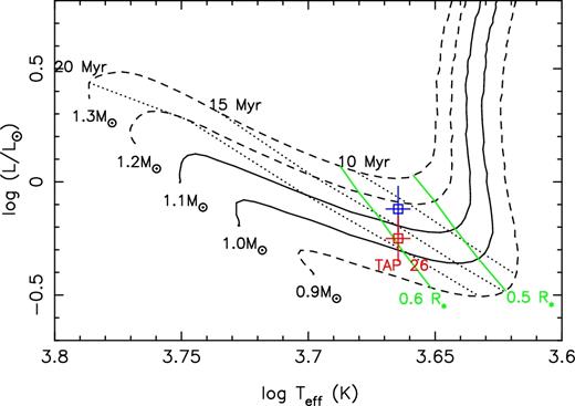
Observed location of TAP 26 in the HR diagram. The red and blue open squares (with 1σ error bars) depict the location of TAP 26 using two different ways of estimating the inclination angle of the rotation axis – with the red one showing our best estimate used throughout the paper. The PMS evolutionary tracks for 0.9, 1.0, 1.1, 1.2 and 1.3 M_⊙, and corresponding isochrones for 10, 15 and 20 Myr (Siess, Dufour & Forestini 2000) assume solar metallicity and include convective overshooting. The green lines depict where models predict PMS stars’ radiative core reaches a radius of 0.5 R_⋆ and 0.6 R_⋆.

Referring to Donati et al. (2015, 2017), TAP 26 closely resembles an evolved version of the 2 Myr star V830 Tau that would have contracted and spun up by 4× towards the zero-age main sequence, with the rotation period and radius of V830 Tau being, respectively, 2.741 d and 2.0 ± 0.2 R_⊙. The increase in rotation rate matches quite well the predicted decrease in the moment of inertia between both epochs according to evolutionary models of Siess et al. (2000). Given the prominent role of the disc in braking the rotation of the star and thus decreasing its angular momentum (Davies, Gregory & Greaves 2014; Gallet & Bouvier 2015), this also suggests that TAP 26 dissipated its accretion disc very early, typically as early as, or earlier than V830 Tau. We also note that our target is located past the theoretical threshold at which stars start to be more than half radiative in radius, suggesting that the magnetic field of TAP 26 already started to evolve into a complex topology (Gregory et al. 2012).

The stellar parameters inferred and used in this study are summarized in Table 3.

Table 3.

Parameters for TAP 26, inferred from the photometric and spectroscopic measurements and the ZDI analysis (see Section 4). Respectively: distance to Earth d, mass M_⋆, radius R_⋆, effective temperature T_eff, decimal logarithm of surface gravity log g, logarithmic luminosity log (L_⋆/L_⊙), age, rotation period P_rot, inclination of the rotation axis to the line of sight i, line-of-sight-projected equatorial rotation velocity vsin i, equatorial rotation rate Ω_eq, difference dΩ between equatorial and polar rotation rates and mean RV in the barycentric rest frame v_rad (which was derived from our spectropolarimetric runs, see Section 4). T09 and G13 in the references, respectively, stand for Torres et al. (2009) and Grankin (2013).

Parameter	Value	Reference
d (pc)	147±3	T09
M⋆ (M⊙)	1.04±0.10
R⋆ (R⊙)	1.17±0.17
Teff (K)	4,620±50
log g	4.5
log (L⋆/L⊙)	−0.25 ±0.10
Age (Myr)	≃17
Prot (d)	0.7135	G13
i (°)	55±10
vsin i (km s−1)	68.2±0.5
Ωeq (rad d−1)	8.8199±0.0003
dΩ (rad d−1)	0.0492±0.0010
vrad (km s−1)	16.25 ± 0.20

4 TOMOGRAPHIC IMAGING

In order to model the activity jitter of TAP 26 (see Section 5), we applied ZDI (Semel 1989; Brown et al. 1991; Donati & Brown 1997) to our data. ZDI takes inspiration from medical tomography, which consists of constraining a 3D distribution using series of 2D projections as seen from various angles (Vogt, Penrod & Hatzes 1987). In our context, ZDI inverts simultaneous time series of 1D Stokes I and V LSD profiles into 2D brightness and magnetic field maps of the stellar surface (see Donati et al. 2014). The magnetic field is decomposed into its poloidal and toroidal components, both expressed as spherical harmonics expansions (Donati et al. 2006).

Synthetic LSD profiles are derived from brightness and magnetic maps by summing up the spectral contribution of all cells, taking into account the Doppler broadening caused by the rotation of the star, the Zeeman effect induced by magnetic fields and the continuum centre-to-limb darkening. Local Stokes I and V profiles are computed using Unno–Rachkovsky's analytical solution to the polarized radiative transfer equations in a Milne–Eddington model atmosphere (Landi degl'Innocenti & Landolfi 2004). The local profile used in this study has a central wavelength, a Doppler width and a Landé factor of typical values 670 nm, 1.8 km s⁻¹ and 1.2, respectively, and an equivalent width of 4.6 km s⁻¹ corresponding to the LSD profiles of TAP 26. Technically, ZDI applies a conjugate gradient technique to iteratively reconstruct the brightness and magnetic surface maps with minimal information content (i.e. maximum Shannon entropy) that matches our observed LSD profiles at a given reduced chi-square (⁠|$\chi ^2_{\rm r}$|⁠, defined as χ² divided by the number of data points²) level. Concerning the brightness, we note that, unlike in Donati & Collier Cameron (1997) where we fit a spot filling factor with pre-set spot parameters, here we fit the local brightness b_k of cell k, relative to the quiet photosphere (0 <b_k < 1 for dark spots and b_k > 1 for bright plages), as described in Donati et al. (2014).

ZDI can also take into account and model latitudinal differential rotation, shearing the brightness distribution and magnetic topology at the surface of the star, and assuming a solar-like surface rotation rate, Ω(θ), varying with latitude, θ, as

\begin{equation} \Omega (\theta )=\Omega _{\rm eq}-\rm d\Omega (\sin \theta )^2, \end{equation}

(2)

where Ω_eq is the equatorial rotation rate and dΩ is the difference between the equatorial and the polar rotation rates.

For a given set of parameters, ZDI looks for the map with minimal information content that matches the LSD profiles at |$\chi ^2_{\rm r}$|= 1. As a by-product, we obtain the optimal stellar parameters for which the reconstructed images contain minimal information: i = 55 ± 10°, vsin i = 68.2 ± 0.5 km s⁻¹ and v_rad= 16.25 ± 0.20 km s⁻¹ (the RV the star would have if unspotted and planet-free). Regarding differential rotation, we obtain Ω_eq= 8.8199 ± 0.0003 rad d⁻¹ and dΩ= 0.0492 ± 0.0010 rad d⁻¹, as outlined in more detail in Section 4.2.

4.1 Brightness and magnetic imaging

Given the long time span between our two data sets (about 60 d, see Table 1), we start by reconstructing separate brightness and magnetic maps for each epoch (2015 November and 2016 January), before investigating the temporal variability between both in more detail.

The Stokes I and V LSD profiles, which are displayed in Fig. 2, were used simultaneously to reconstruct both surface brightness and magnetic field maps. The synthetic LSD profiles presented in the figure match the observed ones at |$\chi ^2_{\rm r}$| = 1, or, equivalently, at a χ² equal to 1484 for the 2015 November data set and 1157 for the 2016 January data set, and for both sets of Stokes I and V LSD profiles. The iterative reconstruction starts from unspotted magnetic maps corresponding to |$\chi ^2_{\rm r}$| = 13 (2015 November) and 9 (2016 January), showing that the iterative algorithm of ZDI successfully manages to reproduce the data at noise level. In the particular case of Stokes I profiles, whose noise includes a significant level of systematics (see Section 2), we find that smaller error bars make ZDI unable to fit the data down to |$\chi ^2_{\rm r}$|= 1; on the opposite, greater error bars result in a fit to the Stokes I profiles for which the raw radial velocities are not properly reproduced (see Section 5). This gives us confidence that the S/N values derived for the Stokes I LSD profiles (see Table 1) are accurate and reliable within 10 per cent.

Figure 2.

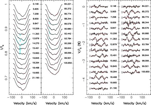
Maximum entropy fit (thin red lines) to the observed (thick black lines) Stokes I (left) and V (right) LSD profiles. The 2015 November data set is represented in the first and third panels and the 2016 January data set in the second and fourth panels. The Stokes I LSD profiles before the removal of lunar pollution are coloured in cyan, and 3σ error bars are displayed for the Stokes V profiles. The rotational cycles are written beside their corresponding profiles, in concordance with Table 1.

The reconstructed brightness maps for 2015 November and 2016 January are shown in Fig. 3, at an epoch corresponding to rotation cycle 10.0 (in the ephemeris of equation 1) for 2015 November, and 92.0 for 2016 January (see Table 1); the colour scale codes the logarithmic relative brightness compared to that of the photosphere. The surface spot coverage we derive is similar at both epochs, reaching 10 per cent in the 2015 November map (5 per cent/5 per cent of cool spots/hot plages, respectively) and 12 per cent in the 2016 January map (7 per cent/5 per cent of cool spots/hot plages, respectively). Both reconstructed maps share some similarities, such as a large cool polar cap resembling that reconstructed on other rapidly rotating wTTSs (e.g. Skelly et al. 2010; Donati et al. 2014), plus a number of smaller features located at lower latitudes (in particular the two equatorial spots located at phases 0.22 and 0.92 in 2015 November, 0.27 and 0.97 in 2016 January) interleaved with bright plages. We stress that ZDI is only sensitive to the medium and large brightness features and misses small spots evenly distributed over the whole stellar surface, implying that the spottedness we recover for TAP26 is likely an underestimate. We observe a number of differences between both images potentially attributable to differential rotation and/or intrinsic variability (see Section 4.2); however, the limited phase coverage at both epochs makes the direct comparison of individual surface features between maps ambiguous and hazardous. We caution that the smallest scale structures may reflect to some extent the limited phase coverage and be subject to phase ghosting (e.g. Stout-Batalha & Vogt 1999).

Figure 3.

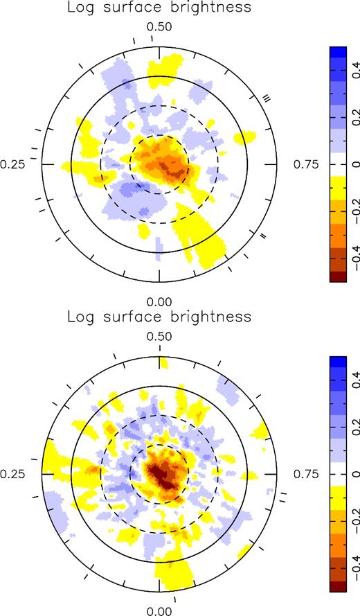
Flattened polar view of the surface-brightness maps for the 2015 November data set (top panel) and 2016 January data set (bottom panel). The equator and the 60°, 30° and −30° latitude parallels are depicted as solid and dashed black lines, respectively. The colour scale indicates the logarithm of the relative brightness, with brown/blue areas representing cool spots/bright plages. Finally, the outer ticks mark the phases of observation.

Using the brightness maps reconstructed with ZDI, we can predict photometric light curves at both epochs, which are found to compare well with our contemporaneous CrAO observations (see Fig. 4). Note the small but significant temporal evolution of the light curve that we predict between both epochs; this variability is however not obvious from the observed photometric data given their limited sampling and comparatively large error bars (rms 16 mmag).

Figure 4.

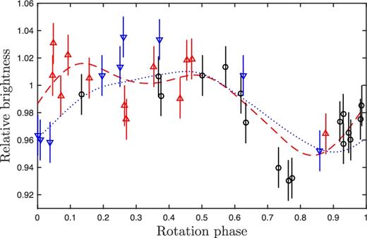
Photometry curves of the relative brightness as function of the rotation phase. The light curves synthesized from the reconstructed brightness maps for 2015 November and 2016 January are represented by a dashed red line and a dotted blue line, respectively. The CrAO measurements are represented as dots with 1σ error bars, with the observations from 2015 August–October in black circles, the observations from 2015 October–December in red upward-pointing triangles and the observations from 2015 December to 2016 March in blue downward-pointing triangles.

The reconstructed magnetic topology is shown in Fig. 5. The large-scale field reconstructed for TAP 26 features an rms magnetic flux of 330 and 430 G in 2015 November and 2016 January, respectively. The field is found to be mainly poloidal (70 per cent of the reconstructed magnetic energy), though with a significant toroidal component (30 per cent of the reconstructed magnetic energy). It is also largely axisymmetric (50 per cent and 80 per cent of the poloidal and the toroidal field energy, respectively).

Figure 5.

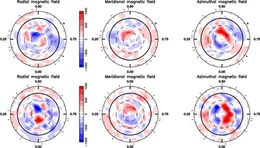
From left to right: radial, meridional and azimuthal component of the surface magnetic field (labelled in G), reconstructed with ZDI from the 2015 November data set (top panels) and the 2016 January data set (bottom panels).

The dipolar component of the large-scale field has a strength of 120 ± 10 G at both epochs, corresponding to about 10 per cent of the reconstructed poloidal field energy, and is tilted at 40 ± 5° to the line of sight, i.e. mid-way to the equator, towards phase 0.73 ± 0.03 and 0.85 ± 0.03 in 2015 November and 2016 January, respectively. The increase in the phase towards which the dipole is tilted suggests that intermediate to high latitudes (at which the dipole poles are anchored) are rotating more slowly than average by 0.19 per cent, i.e. with a period of ≃0.7148 d; this is confirmed by the fact that the line-of-sight-projected (longitudinal) magnetic field B_ℓ (proportional to the first moment of the Stokes V profiles, e.g. Donati et al. 1997, and most sensitive to the low-order components of the large-scale field) exhibits a recurrence time-scale of 1.0014 ± 0.003 P_rot (see Appendix B), i.e. slightly longer than P_rot by a similar amount. Higher order terms in the spherical harmonics expansion describing the field (in particular the quadrupolar and octupolar modes) get stronger between 2015 November and 2016 December, with total magnetic energies increasing from 85 per cent to 93 per cent of the poloidal field.

Finally, we show a large-scale extrapolation of the magnetic field (under the assumption of a potential field) in Fig. 6. Similarly to the brightness maps, the magnetic maps seem to point to a variation of the surface topology between late 2015 and early 2016, which is not explained by differential rotation alone, though the limited phase coverage calls for caution when comparing features between those maps.

Figure 6.

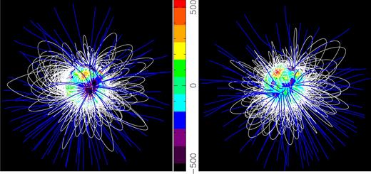
Potential field extrapolations of the reconstructed magnetic topology as seen by an Earth-based observer, in 2015 November (left) and in 2016 January (right) both at phase 0.8. Open and closed field lines are shown in blue and white, respectively, whereas colours at the stellar surface depict the local value of the radial field (in G, as shown in the left-hand panels of Fig. 5). The source surface at which the field becomes radial is set to 4 R_⋆, slightly larger than the corotation radius of about 3 R_⋆ (at which the Keplerian period equals the stellar rotation period) and beyond which field lines are expected to quickly open under centrifugal forces.

The magnetic maps suggest that the magnetic topology at the rotation pole underwent a ≃0.1 phase shift between both dates.

4.2 Intrinsic variability and differential rotation

When applying ZDI to the whole data set, i.e. modelling all Stokes I and V profiles with only one brightness map and one magnetic topology (see Appendix A), we obtain a minimum |$\chi ^2_{\rm r}$| value of 1.4, even when taking into account differential rotation (starting from an initial value |$\chi ^2_{\rm r}$|= 20). This indicates that intrinsic variability occurred during the 45 d gap (or 63 rotation cycles) separating both data sets.

Despite this variability, we attempted to retrieve differential rotation from the whole data set. The search for differential rotation parameters is done by minimizing the value of |$\chi ^2_{\rm r}$| at a fixed amount of information, in this present case using the Stokes I profiles and brightness map reconstruction only. From the curvature of the |$\chi ^2_{\rm r}$| paraboloid around the minimum, one can infer error bars on differential rotation parameters (Donati, Collier Cameron & Petit 2003). The spot coverage is fixed at 13 per cent (chosen to be slightly higher than the values found in each reconstruction) and the values we found are Ω_eq= 8.8199 ± 0.0003 rad d⁻¹ and dΩ = 0.0492 ± 0.0010 rad d⁻¹, with a minimum |$\chi ^2_{\rm r}$| of 1.4116. A map of Δχ² is shown in Fig. 7, which presents a very clear paraboloid around the minimum we found, even if, due to our phase coverage, these precise values ask for further confirmation with the help of future data. This value of dΩ is close to the solar differential rotation (0.055 rad d⁻¹). The case with no differential rotation yields |$\chi ^2_{\rm r}$| = 2.6907. Normalizing Δχ² by the minimum χ² achieved over the map (to scale up error bars as a way to account for the contribution from the reported intrinsic variability) still yields a value in excess of 3300 and a negligible false alarm probability (FAP), unambiguously demonstrating that the star is not rotating as a solid body.

Figure 7.

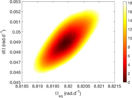
Map of Δχ² as a function of Ω_eq and dΩ, derived from the modelling of our Stokes I LSD profiles of TAP 26 at constant information content. A well-defined paraboloid is observed with the outer colour contour corresponding to the 99.99 per cent confidence level area (i.e. a χ² increase of 18.4 for the 2581 Stokes I data points). The minimum value of |$\chi ^2_{\rm r}$| is 1.4116. The minimum |$\chi ^2_{\rm r}$| achieved is above unity due to intrinsic variability affecting the LSD profiles but not being taken into account within ZDI. The derived differential rotation parameters are Ω_eq = 8.8199 ± 0.0003 rad d⁻¹ and dΩ = 0.0492 ± 0.0010 rad d⁻¹.

The differential rotation parameters we obtain imply a lap time of 128 ± 3 d, with rotation periods of 0.712 39 ± 0.000 03 d and 0.716 38 ± 0.000 08 d for the equator and pole, respectively, in good agreement with the range of rotation periods derived from photometry (ranging from 0.7135 to 0.7138, Grankin 2013). The 0.7132 d period found for the equivalent width of the Hα line and the 0.7145 d period found for the longitudinal magnetic field B_ℓ (see Appendix B) are also consistent. We note that the rotation periods found with photometry, the longitudinal magnetic field and Hα line correspond to latitudes ranging from 30° to 50°, indicating that an important amount of activity is concentrated at these mid-latitudes, with the dipole pole located in the upper part of this range, in good agreement with the ZDI reconstruction (see Section 4.1).

5 MODELLING THE PLANET SIGNAL

We describe below three different techniques aimed at characterizing the RV curve of TAP 26. The first two are those used in Donati et al. (2017): filtering out the activity modelled with the help of ZDI, and the simultaneous fit of the planet parameters and the stellar activity. The third method follows the approach of Haywood et al. (2014) and Rajpaul et al. (2015) and uses GPR to model the activity directly from the raw RVs. The results obtained from these three methods are outlined and discussed in the following sections.

5.1 Jitter activity filtering

The first technique consists of using the previously reconstructed maps to predict the pollution to the RV curve caused by activity (called activity jitter in the following) and subtract it from the raw RVs. From the observed Stokes I LSD profiles, we compute, at both epochs, the raw RVs RV_raw (and error bars, see Table 1), as the first-order moment of the continuum-subtracted corresponding profiles (Donati et al. 2017). Likewise, the synthesized Stokes I LSD profiles derived from the brightness maps yield the synthesized activity jitter of the star (RV signal caused by the brightness distribution and stellar rotation). By subtracting the activity jitter from the raw RVs, we obtain filtered RVs RV_filt (see Table 1). We observe that the jitter has a mean semi-amplitude of 1.81 km s⁻¹ in 2015 November and 1.21 km s⁻¹ in 2016 January, whereas the filtered RV curve features a signal with a semi-amplitude of ≃0.15 km s⁻¹ (Fig. 8), i.e. 8 to 12 times smaller than the activity signal we filtered out. We note the very significant evolution in the activity curve between 2015 November and 2016 January, demonstrating that the brightness distribution has evolved at the surface of TAP 26, through differential rotation and intrinsic variability (see Section 4).

Figure 8.

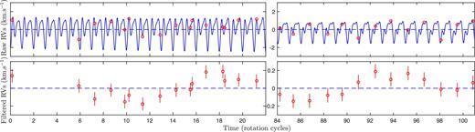
Top panels: RV (in the stellar rest frame) of TAP 26 as a function of rotation phase, as measured from our observations (open circles) and predicted by the tomographic maps (blue line). The synthesized raw RV curves exhibit only low-level temporal evolution resulting from differential rotation. Bottom panels: filtered RVs derived by subtracting the modelled activity jitter from the raw RVs, with a 10× zoom-in on the vertical axis.

With an rms dispersion of 109 m s⁻¹, the filtered RVs clearly show the presence of a signal. Looking for a planet signature, we want to fit a sine curve (of semi-amplitude K, period P_orb, phase of inferior conjunction ϕ and offset RV₀) to these filtered RVs, which corresponds to a circular orbit (see Fig. 9). The phase of inferior conjunction, i.e. corresponding to the epoch at which the planet is closest to us, is defined relatively to the reference date BJD_c0 = 2457352.6485 (rotation cycle 11.0, approximately at the centre of the 2015 November observation run), such that the inferior conjunction occurs at BJD_c= BJD_c0 + (ϕ −1)P_orb. Due to the gap between both observing runs, several sine fits with different frequencies match the RV_filt as local minima of |$\chi ^2_{\rm r}$|⁠. The four best fits are shown in Fig. 9 and their characteristics are given in Table 4, with the value of the log likelihood as computed from the Δχ² over these 29 RV data points. The residual RVs, derived from subtracting the best sine fit to the filtered RVs (shown in Fig. 9), feature an rms value of 51 m s⁻¹.

Figure 9.

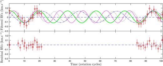
Top: filtered RVs of TAP 26 and four sine curves representing the best fits. The thick green curve represents the case P_orb/P_rot = 18.80, the thin magenta one P_orb/P_rot = 15.27, the dash–dotted blue one P_orb/P_rot = 24.56 and the dotted black one P_orb/P_rot = 12.76. Bottom: residual RVs resulting from the subtraction of the best fit (green curve) from the filtered RVs. The residual RVs feature an rms value of 51 m s⁻¹.

Table 4.

Characteristics of the four best sine curve fits to the filtered RVs, and the case without planet. Respectively: semi-amplitude K, orbital period P_orb in units of P_rot, orbital period P_orb in days, phase of inferior conjunction ϕ relative to cycle 11.0 (see ephemeris in equation 1), BJD of inferior conjunction, RV offset RV₀, corresponding |$\chi ^2_{\rm r}$|⁠, difference in χ² with the best fit (Δχ², summed on the 29 data points) and natural logarithm (log_e) of the likelihood |$\mathcal {L}_{r1}$| relative to the best fit. ϕ relates to the epoch of inferior conjunction BJD_c through BJD_c=2457352.6485+ϕP_orb, the reference date being chosen so as to minimize the variation of ϕ between the four cases.

K	Porb	Porb	ϕ	BJDc	RV0	|$\chi ^2_{\rm r}$|	Δχ2	|$\log \mathcal {L}_{r1}$|	Style
(km s−1)	(Prot)	(d)		(2457340+)	(km s−1)				in Fig. 9
0.131±0.020	18.80±0.23	13.41±0.16	0.709±0.026	8.75±0.35	0.009±0.014	0.445	0	0.00	Thick green
0.133±0.021	15.27±0.14	10.90±0.10	0.715±0.024	9.54±0.26	0.012±0.014	0.542	2.80	−0.53	Full magenta
0.124±0.020	24.56±0.41	17.52±0.30	0.684±0.028	7.11±0.50	0.009±0.016	0.673	6.61	−1.85	Dash-dotted blue
0.107±0.021	12.76±0.14	9.11±0.10	0.724±0.031	10.14±0.28	0.018±0.015	1.079	18.38	−6.87	Dotted black
0					0.013±0.014	2.025	45.82	−19.73	Dashed blue

Plotting Lomb–Scargle periodograms for the raw RVs, filtered RVs and residual RVs further demonstrates the presence of a periodic signal in the filtered RVs (Fig. 10). The above-mentioned dominant periods are seen as peaks in the periodogram; periodograms of partial data (only the 2015 November data set, only the 2016 January data set, odd points and even points) are also shown, yielding peaks at the same frequencies albeit with a lower power. We highlight the fact that the highest peaks in the raw RVs correspond to the activity jitter and are located at P_rot/2 and its aliases, whereas little power concentrates at P_rot itself. A zoom-in of the filtered RV periodogram is also shown in Fig. 10 (bottom panel). The FAP is 0.06 per cent for the highest peak (P_orb = 13.41 d = 18.80 P_rot), and no significant period stands out in the residual RVs after filtering out both the activity jitter and the planet signal corresponding to the highest peak. We carried out simulations to ensure that the detected peaks are not generated by the filtering process, see details in Appendix C. Study of other activity proxies shows that the detected orbital periods are not present in the activity signal either (Appendix B).

Figure 10.

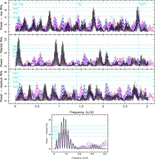
Top: periodograms of the raw (top), filtered (middle) and residual (bottom) RV curves over the whole data set (black line). The red line represents the 2015 November data set, the green line the 2016 January data set, the blue line the odd data points and the magenta line the even data points. FAP levels of 0.33 and 0.10 are displayed as horizontal dotted cyan lines, FAP levels of 0.03 and 0.01 are displayed as horizontal dashed cyan lines. The rotation frequency (1.402 cycles d⁻¹) is marked by a vertical cyan dashed line, as well as its first harmonic (2.803 cycles d⁻¹) and the orbital frequency that has the smallest FAP (0.06 per cent at 0.075 cycles d⁻¹, corresponding to P_orb=13.41 d). Aliases of the highest peaks, related to the observation window, appear as lower peaks separated by one cycle per day. Bottom: zoom-in the periodogram of filtered RVs.

By fitting the filtered RVs with a Keplerian orbit rather than a circular orbit, we obtain an eccentricity of 0.16 ± 0.15, indicating that there is no evidence for an eccentric orbit (following the precepts of Lucy & Sweeney 1971). We can thus conclude that the orbit of TAP 26 b is likely close to circular, or no more than moderately eccentric.

5.2 Deriving the planetary parameters from the LSD profiles

A second technique, following the method of Petit et al. (2015), consists of taking into account the presence of a planet into the ZDI model. Rather than fitting the measured Stokes I LSD profiles with a synthetic activity jitter directly, we first apply a translation in velocity to each of them, to remove the reflex motion caused by a planet of given parameters, and then apply ZDI to the corrected data set. Practically speaking, we repeat the experiment for a range of values for the orbital parameters (K, P_orb, ϕ) at the vicinity of the minima previously identified in Section 5.1 and look for the set of values that yields the best result. The same way as for differential rotation, we derive the error bars on all parameters from the curvature of the 3D |$\chi ^2_{\rm r}$| paraboloid around the minimum.

In the present case, since we have two data sets separated by a 45 d gap and we know that intrinsic variability occurred (see Sections 4 and 5.1), a modification to the method described above was implemented: after correcting the global data set from the reflex motion, ZDI is applied separately on each data set, reconstructing two different brightness maps (one for late 2015 and one for early 2016) in order to obtain a more precise reconstruction. The quantity used to measure the likelihood of each set of parameters is therefore a global |$\chi ^2_{\rm r}$|⁠, computed as a weighted average of both individual |$\chi ^2_{\rm r}$|⁠, with respective weights proportional to the number of data points in each set (1424 for 2015 November and 1157 for 2016 January).

As in the previous section, several minima are found, which are listed in Table 5. We also computed the relative likelihood of each case compared to the best one from the corresponding difference in |$\chi ^2_{\rm r}$|⁠. We note that the case with no planet yields |$\chi ^2_{\rm r}$| = 0.98631, which leads to a relative probability lower than 10⁻⁹ compared to the case with a 10.91 d period planet.

Table 5.

Optimal orbital parameters derived with the method described in Section 5.2, respectively: semi-amplitude K, orbital period P_orb in units of P_rot, orbital period P_orb in days, phase of inferior conjunction ϕ relative to cycle 11.0, BJD of inferior conjunction, |$\chi ^2_{\rm r}$|⁠, Δχ² summed on 2581 data points, and natural logarithm of the likelihood |$\mathcal {L}_{r2}$| relative to the best fit. The case where no planet is taken into account in the model is given for comparison.

K	Porb	Porb	ϕ	BJDc	|$\chi ^2_{\rm r}$|	Δχ2	|$\log \mathcal {L}_{r2}$|
(km s−1)	(Prot)	(d)		(2457340+)
0.154±0.022	15.29±0.15	10.91±0.11	0.671±0.035	9.06±0.38	0.968 24	0.00	0.00
0.144±0.023	18.78±0.25	13.40±0.18	0.685±0.041	8.43±0.55	0.969 79	4.00	−1.34
0.148±0.025	12.83±0.12	9.16±0.09	0.677±0.038	9.69±0.35	0.971 80	9.17	−3.61
0					0.986 31	46.62	−21.60

Fig. 11 displays a Δχ² map around the local minimum P_orb/P_rot= 15.29, at ϕ = 0.67, showing the 99.99 per cent confidence area.

Figure 11.

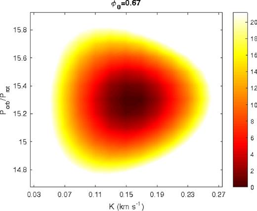
Δχ² map as a function of K and P_orb/P_rot, derived with ZDI from corrected Stokes I LSD profiles at constant information content. Here the phase is fixed at 0.67, i.e. the value of ϕ at which the 3D paraboloid is minimum. The outer colour delimits the 99.99 per cent confidence level area (corresponding to a χ² increase of 21.10 for 2581 data points in our Stokes I LSD profiles). The minimum value of |$\chi ^2_{\rm r}$| is 0.968 24.

5.3 Gaussian-process regression (GPR)

The third method we used works directly with the raw RVs and aims at modelling the activity jitter and its temporal evolution with GPR, assuming it obeys an a priori covariance function (Haywood et al. 2014; Rajpaul et al. 2015). Similarly to the previous method, we fit both the orbit model and the jitter model simultaneously. For a planet with given parameters, we first remove the planet reflex motion from the RVs, then we fit the corrected RVs with a Gaussian process (GP) of pseudo-periodic covariance function:

\begin{equation} c(t,t^{\prime })=\theta _1^2\exp \left[-\frac{(t-t^{\prime })^2}{\theta _3^2}-\frac{\sin ^2\left(\frac{\pi (t-t^{\prime })}{\theta _2}\right)}{\theta _4^2}\right], \end{equation}

(3)

where t and t΄ are two dates, θ₁ is the amplitude (in km s⁻¹) of the GP, θ₂ the recurrence time-scale (in units of P_rot), θ₃ the decay time-scale (i.e. the typical spot lifetime in the present case, in units of P_rot) and θ₄ a smoothing parameter (within [0,1]) setting the amount of high-frequency structures that we allow the fit to include. From a given set of orbital parameters (K, P_orb, ϕ) and of covariance function parameters (θ₁ to θ₄, called hyperparameters), we can derive the GP that best fits the corrected RVs (noted y below) as well as the log likelihood |$\log \mathcal {L}$| of the corresponding set of parameters from

\begin{equation} 2\log \mathcal {L}=-n\log (2\pi )-\log |C+\Sigma |-y^T(C+\Sigma )^{-1}y, \end{equation}

(4)

where n is the number of data points (29 in our case), C is the covariance matrix of all the observing epochs and Σ is the diagonal variance matrix of the raw RVs.

Coupled with a Markov Chain Monte Carlo (MCMC) simulation to explore the parameter domain, this method generates samples from the posterior probability distributions for the hyperparameters of the noise model and the orbital parameters. From these we can determine the maximum-likelihood values of these parameters and their uncertainty ranges. After an initial run where all the parameters are free to vary, we fix θ₄ and θ₃ to their respective best values (0.50 ± 0.09 and 180 ± 60 P_rot = 128 ± 43 d) before carrying out the main MCMC run to find the best estimates of the five remaining parameters. We note that the best value found for the decay time is exactly equal to the differential rotation lap time within error bars, and to twice the total span of our data. This decay time corresponds to both the differential rotation lap time and the star-spot coherence time, since these are the most influent phenomena on the periodicity of the activity jitter. Such a star-spot coherence time is consistent with previous studies (Lanza 2006; Grankin et al. 2008; Bradshaw & Hartigan 2014).

As shown in Fig. 12, this method successfully recovers the different minima previously found with the first two techniques, with little correlation between the various parameters thus minimum bias in the derived values. Applying the method of Chib & Jeliazkov (2001) to the MCMC posterior samples, we obtain that the marginal likelihood of the case P_orb = 12.61 P_rot is larger than that of the case P_orb = 15.12 P_rot by a Bayes factor of only 1.28, which implies that there is as yet no clear evidence in favour of either of them. The third most likely case, P_orb= 18.74 P_rot, has a marginal likelihood which is inferior to the first one by a Bayes’ factor of >8, and the case with no planet has a marginal likelihood which is smaller than that of the first case by a Bayes factor of 2 × 10⁵. The three most likely sets of parameters are summarized in Table 6.

Figure 12.

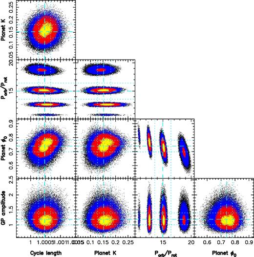
Phase plots of our 5-parameter MCMC run with yellow, red and blue points marking, respectively, the 1σ, 2σ and 3σ confidence regions. The optimal values found for each parameters are: θ₁ = 1.19 ± 0.21 km s⁻¹, θ₂ = 1.0005 ± 0.0002 P_rot, K = 0.152 ± 0.029 km s⁻¹. Several optima are detected for P_orb: 12.61 ± 0.13 P_rot, 15.12 ± 0.20 P_rot and 18.74 ± 0.34 P_rot, ordered by decreasing likelihood. The corresponding phases ϕ are 0.766 ± 0.030, 0.728 ± 0.033 and 0.694 ± 0.042, respectively.

Table 6.

Sets of orbital parameters that allow us to fit the corrected RV curve best, using a GP with a covariance function given in equation (4), derived from the MCMC run. Respectively: reflex motion RV semi-amplitude K, orbital period P_orb in units of P_rot, orbital period P_orb in days, phase of inferior conjunction ϕ relative to rotation cycle 11.00 (ephemeris defined in equation 1), BJD of inferior conjunction, natural logarithm of the marginal likelihood |$\mathcal {L}$| and natural logarithm of the relative marginal likelihood |$\mathcal {L}_{r3}$| as compared to the best case. The case where no planet is taken into account in the model is given for comparison.

K	Porb	Porb	ϕ	BJDc	|$\log \mathcal {L}$|	|$\log \mathcal {L}_{r3}$|
(km s−1)	(Prot)	(d)		(2457340+)
0.163	12.61	8.99	0.766	10.54	−3.48	0.00
±0.028	±0.13	±0.09	±0.030	±0.27
0.149	15.12	10.79	0.728	9.71	−3.73	−0.25
±0.026	±0.20	±0.14	±0.033	±0.36
0.139	18.74	13.37	0.694	8.56	−5.60	−2.12
±0.026	±0.34	±0.24	±0.042	±0.57
0					−15.80	−12.52

Trying to fit a non-circular Keplerian orbit to our data, i.e. adding the periapsis argument and the eccentricity e to the parameters in our MCMC run, we obtain e = 0.05 ± 0.18, with a marginal likelihood slightly smaller than that of the case of a circular orbit. This further supports that the planet eccentricity is low if non-zero.

The best fit with our third method is shown in Fig. 13, where we see the raw RVs and the modelled RV curve predicted with this method, i.e. the sum of the GPR-fitted activity jitter and of the planet signal. Zooming in shows that this curve presents similarities with the RV jitter curve derived by ZDI (Fig. 8), indicating that, although working only with the RV data points, GPR successfully retrieves a convincing model for the activity. We also note the ability of the GP to model the activity jitter not only during our observing runs, but also during the 45 d gap between them, emphasizing the variability of the RV signal with time. The residual RVs in the case presented here have an rms value of 29 m s⁻¹ (close to the instrument RV precision 20–30 m s⁻¹) whereas the residual RVs derived with the first method yield an rms value of 51 m s⁻¹. Though the rms value is 2.5 times smaller than the error bar, GPR only fits two parameters, which illustrates its flexibility without decreasing its reliability, since the results are consistent with those found using independent methods (Sections 5.1 and 5.2). This demonstrates that GPR does a better job at modelling the activity jitter and its temporal evolution than the two previous methods, in agreement with the conclusions of Donati et al. (2016) in the case of the wTTS V830 Tau. As a result, we consider the optimal planet parameters derived with GPR as the most reliable ones, and therefore conclude that the orbital periods of 10.8 and 9.0 d are more or less equally likely.

Figure 13.

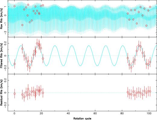
RV curves for a GPR fit of the activity jitter, with parameters K = 0.163 km s⁻¹, P_orb= 12.61 P_rot, ϕ = 0.766, θ₁ = 1.19 km s⁻¹, θ₂ = 1.0005 P_rot, θ₃ = 180 P_rot, θ₄ = 0.50 P_rot. Top panel: raw RVs and their error bars are shown in red, the solid cyan curve is the sum of the activity jitter predicted by GPR and the planet signal, and the dashed cyan lines show the 68.3 per cent confidence intervals about the prediction around this model. Middle panel: filtered RVs and their error bars, resulting from the subtraction of the GP-fitted activity jitter from the raw RVs (in red), and the sine curve corresponding to the assumed planet signal (in cyan). Bottom panel: residual RVs resulting from the subtraction of the planet signal from the filtered RVs, and their error bars. The residual RVs feature an rms value of 29 m s⁻¹, i.e. the GP fits the RVs down to |$\chi ^2_{\rm r}$| = 0.151.

Table 7 summarizes the likelihood of the different periods found with each method.

Table 7.

Results yielded by the methods ZDI no. 1 (Section 5.1), ZDI no. 2 (Section 5.2) and GPR (Section 5.3), for the two periods ≃15 P_rot and ≃13 P_rot. From top to bottom: reflex motion semi-amplitude K, phase of inferior conjunction ϕ relative to cycle 11.0, orbital period P_orb in units of P_rot, orbital period P_orb in days, semimajor axis a, Msin i in units of Jovian mass, BJD of inferior conjunction BJD_c, natural logarithm of relative likelihood as compared to the best case |$\mathcal {L}_{r}$|⁠, GP amplitude θ₁ and GP recurrence time-scale θ₂. Results are displayed in bold font when the period is found with the highest likelihood using the corresponding method.

	ZDI no. 1	ZDI no. 2	GPR
K (km s−1)	0.133±0.021	0.154±0.022	0.149±0.026
ϕ	0.715±0.024	0.671±0.035	0.728±0.033
Porb (Prot)	15.27±0.14	15.29±0.15	15.12±0.20
Porb (d)	10.90±0.10	10.91±0.11	10.79±0.14
a (au)	0.0974±0.0032	0.0975±0.0032	0.0968±0.0032
Msin i (MJup)	1.49±0.25	1.73±0.27	1.66±0.31
BJDc (2457340+)	9.54±0.26	9.06±0.38	9.71±0.36
|$\log \mathcal {L}_r$|	−0.53	0.00	−0.25
θ1 (km s−1)			1.19±0.21
θ2 (Prot)			1.0004±0.0002
K (km s−1)	0.107±0.021	0.148±0.025	0.163±0.028
ϕ	0.724±0.031	0.677±0.038	0.766±0.030
Porb (Prot)	12.76±0.14	12.83±0.12	12.61±0.13
Porb (d)	9.11±0.10	9.16±0.09	8.99±0.09
a (au)	0.0864±0.0028	0.0868±0.0028	0.0858±0.0028
Msin i (MJup)	1.13±0.23	1.56±0.28	1.71±0.31
BJDc (2457340+)	10.14±0.28	9.69±0.35	10.54±0.27
|$\log \mathcal {L}_r$|	−6.87	−3.61	0.00
θ1 (km s−1)			1.19±0.21
θ2 (Prot)			1.0005±0.0002

6 Summary AND discussion

This paper reports the results of an extended spectropolarimetric run on the wTTS TAP 26, carried out within the framework of the international MaTYSSE Large Programme, using the echelle spectropolarimeter ESPaDOnS at CFHT, spanning 72 d from 2015 November 18 to 2015 December 03 then from 2016 January 17 to 29, and complemented by contemporaneous photometric observations from the 1.25-m telescope at CrAO.

Applying ZDI to our two data sets, we derived the surface brightness and magnetic maps of TAP 26, revealing the presence of cool spots and warm plages totalling up to 12 per cent of the stellar surface (we however caution that this is a lower limit given the insensitivity of ZDI to small spots evenly spread over the stellar surface). The large-scale field of TAP 26 is found to be mainly poloidal and axisymmetric, with a 120 G dipole component tilted at 40° from the rotation axis. The 2015 November and 2016 January maps are mostly similar, but none the less feature some differences that indicate temporal evolution of the surface brightness and the magnetic field, demonstrated by the inability of ZDI to model the whole data set at noise level, on a time-scale comparable to that spanning our sample (72 d). ZDI also enabled us to detect the differential rotation pattern at the surface of TAP 26, with dΩ = 0.0492 ± 0.0010 rad d⁻¹, a value close to that of the Sun, implying a time for the equator to lap the pole by one rotation equal to 128 ± 3 d.

We then applied three different methods to search for a planetary signature in the observed spectra. The first method studies the radial velocities filtered out from the activity jitter predicted by ZDI. Our second method looks for the planet parameters that enable the best fit to the corrected LSD profiles, in a way similar to that used to estimate surface differential rotation. The third method uses GPR to fit the activity jitter in the raw RVs, and like the second method, searches for the orbital parameters that enable GPR to fit the raw RVs corrected from the reflex motion best. We find that GPR succeeds best at modelling the intrinsic variability occurring at the surface of TAP 26, and is able to fit raw RVs at an rms precision of 29 m s⁻¹, i.e. close to the instrumental precision of ESPaDOnS (20–30 m s⁻¹, Moutou et al. 2007; Donati et al. 2008) and 30 per cent better than with our first method (yielding an rms precision of 51 m s⁻¹). A similarly low rms was reached by GPR in the study of wTTS V830 Tau (35–37 m s⁻¹, Donati et al. 2017).

All three methods demonstrate the clear presence of a planet signature in the data, although the gap between both data sets generates aliasing problems, causing multiple nearby peaks to stand out in the periodogram. Of the dominant periods, the 10.8 d one emerges strongly for all three methods. It is the most likely with the second method, and equally likely as other periods when using the first and third methods (13.4 and 9.0 d, respectively). Although the 9.0 d orbital period ranks low (and in particular lower than the 13.4 d period) with our first and second methods, we none the less consider it as the second most likely given its first rank with GPR; the most probable explanation for this apparent discrepancy lies in the higher ability of GPR at modelling intrinsic variability of the activity jitter plaguing the RV curve. Allowing ZDI to model temporal evolution of spot distributions and magnetic topologies should bring all methods on an equal footing; this upgrade is planned for a forthcoming study.

Assuming the 10.79±0.14 d period is the true orbital period, and using the values yielded by GPR for K and ϕ, we find a circular orbit of semimajor axis a = 0.0968 ± 0.0032 au = 17.8 ± 2.7 R_⋆, epoch of inferior conjunction BJD_c = 2457349.71 ± 0.36 and Msin i = 1.66 ± 0.31 M_Jup. If the orbital plane is aligned with the equatorial plane of TAP 26, with an assumed inclination of 55°, we obtain a mass M = 2.03 ± 0.46 M_Jup for TAP 26 b. The 8.99 ± 0.09 d period leads to a = 0.086 ± 0.003 au, BJD_c = 2457350.54 ± 0.27 and Msin i = 1.71 ± 0.31 M_Jup.

With an age of ≃17 Myr, TAP 26 is already an aging T Tauri star and on the verge of becoming a post T Tauri star, as demonstrated by its complex geometry and weaker dipole field component (consistent with TAP 26 having a mostly radiative interior). Akin to V830 Tau b (Donati et al. 2017), the hJ in a nearly circular orbit that we have discovered in the young system TAP 26 is better explained by type II disc migration than by planet–planet scattering coupled to tidal circularization. When compared to V830 Tau, a 2 Myr wTTS of similar mass (Donati et al. 2015, 2016, 2017), appears as an evolved version, rotating 4× faster than its younger sister, likely as a direct consequence of its 4× smaller moment of inertia (according to the evolutionary models of Siess et al. 2000).

Regarding the hJs we detected around TAP 26 and V830 Tau and despite their differences (in mass in particular), it would be tempting to claim that, like its host star, TAP 26 b is an evolved version of V830 Tau b. This would actually imply that TAP 26 b migrated outwards under tidal forces from a distance of ≃0.057 au (where V830 Tau b is located) to its current orbital distance of 0.094 au, as a result of the spin period of TAP 26 being ≃ 15 × shorter than the orbital period of TAP 26 b. This option seems however unlikely given the latest predictions of tidal interactions between a young T Tauri star and its close-in hJ (Bolmont & Mathis 2016), indicating that tidal forces can only have a significant impact on an hJ within 0.06 au of a solar-mass host star (for a typical TTS with a radius of ≃2 R_⊙). The most likely explanation we see is thus that TAP 26 b:

• ended up its type-II migration in the accretion disc at the current orbital distance, when TAP 26 was still young, fully convective and hosting a large-scale dipole field of a few kG similar to that of AA Tau (Donati et al. 2010), i.e. strong enough to disrupt the disc up to a distance of 0.09 au;

• was left over once the disc has dissipated at an age significantly smaller than 2 Myr, i.e. before the large-scale field had time to evolve into a weaker and more complex topology, and the inner accretion disc to creep in as a result of the decreasing large-scale field and the subsequent chaotic accretion (e.g. Blinova, Romanova & Lovelace 2016).

Admittedly, this scenario requires favourable conditions to operate; in particular, it needs the accretion disc to vanish in less than 2 Myr, which happens to occur in no more than 10 per cent of single T Tauri stars in Taurus (Kraus et al. 2012). In fact, since both TAP 26 and V830 Tau have the same angular momentum content, it is quite likely that TAP 26 indeed dissipated its disc very early (see Section 3). Quantitatively speaking, assuming (i) that the hJ we detected tracks the location of the inner disc when the disc dissipated, (ii) that the spin period at this time was locked on the Keplerian period of the inner disc (equal to the orbital period of the detected hJ) and (iii) that stellar angular momentum was conserved since then, we derive that the disc must have dissipated when TAP 26 was about three times larger in radius, at an age of less than 1 Myr (according to Siess et al. 2000). Generating a magnetospheric cavity of the adequate size (0.085–0.097 au depending on the orbital period) would have required TAP 26 to host at this time a large-scale dipole field of 0.3–1.0 kG for mass accretion rates in the range 10⁻⁹–10⁻⁸ M_⊙ yr⁻¹, compatible with the large-scale fields found in cTTSs of similar masses (e.g. GQ Lup, Donati et al. 2012).

Along with other recent reports of close-in giant planets (or planet candidates) detected (or claimed) around young stars (van Eyken et al. 2012; David et al. 2016; Donati et al. 2016, 2017; Johns-Krull et al. 2016; Mann et al. 2016), our result may suggest a surprisingly high frequency of hJs around young solar-type stars, with respect to that around more evolved stars (≃1 per cent, Wright et al. 2012). However, this may actually reflect no more than a selection bias in the observation samples (as for their mature equivalents in the early times of velocimetric planet detections). Planets are obviously much easier to detect around non-accreting TTSs as a result of their lower level of intrinsic variability; observation samples (like that of MaTYSSE) are thus naturally driven towards young TTSs whose accretion discs vanished early, i.e. at a time when their large-scale fields were still strong and their magnetospheric gaps large, and thus for which hJs had more chances to survive type-II migration. A more definite conclusion must wait for a complete analysis of the full MaTYSSE sample.

More observations of TAP 26, featuring in particular a more regular temporal sampling, are currently being planned to better determine the characteristics of the newborn hJ we detected. Furthermore, analysing thoroughly the full MaTYSSE data set to pin down the frequency of newborn hJs within the sample observed so far will bring a clearer view on how the formation and migration of young giant planets is occurring. Ultimately, only a full-scale planet survey of young TTSs such as that to be carried out with SpectroPolarimètre InfraRouge, the new generation spectropolarimeter currently being built for CFHT and scheduled for first light in 2018, will be able to bring a consistent picture of how young close-in planets form and migrate, how their population relates to that of mature hJs, and more generally how young hJs impact the formation and early architecture of planetary systems like our Solar system.

Acknowledgments

This paper is based on observations obtained at the Canada–France–Hawaii Telescope (CFHT), operated by the National Research Council of Canada, the Institut National des Sciences de l'Univers of the Centre National de la Recherche Scientifique (INSU/CNRS) of France and the University of Hawaii. We thank the CFHT QSO team for the great work and effort at collecting the high-quality MaTYSSE data presented in this paper. MaTYSSE is an international collaborative research programme involving experts from more than 10 different countries (France, Canada, Brazil, Taiwan, UK, Russia, Chile, USA, Ireland, Switzerland, Portugal, China and Italy). We also warmly thank the IDEX initiative at Université Fédérale Toulouse Midi-Pyrénées (UFTMiP) for funding the STEPS collaboration program between IRAP/OMP and ESO. We acknowledge funding from the LabEx OSUG@2020 that allowed purchasing the ProLine PL230 CCD imaging system installed on the 1.25-m telescope at CrAO. SGG acknowledges support from the Science and Technology Facilities Council (STFC) via an Ernest Rutherford Fellowship [ST/J003255/1]. SHPA acknowledges financial support from CNPq, CAPES and Fapemig. We would also like to acknowledge the Centre de Données Astronomiques de Strasbourg for the SIMBAD data base.

1

Spot coverage: integral of the difference between local brightness and photosphere brightness over the surface of the star, in units of photosphere brightness.

2

This follows the usual convention in regularized tomographic imaging techniques, where the number of model parameters is much smaller than the number of fitted data points and not taken into account in the expression of |$\chi ^2_{\rm r}$| (Donati et al. 2017).

SUPPORTING INFORMATION

Supplementary data are available at MNRAS online.

tap26_2016_sub3_online.pdf

Please note: Oxford University Press is not responsible for the content or functionality of any supporting materials supplied by the authors. Any queries (other than missing material) should be directed to the corresponding author for the article.

APPENDIX A: ADDITIONAL FIGURES

Images of brightness and magnetic field on the surface of TAP 26, as derived with ZDI using our 29 spectra, are shown in Fig. A1.

Figure A1.

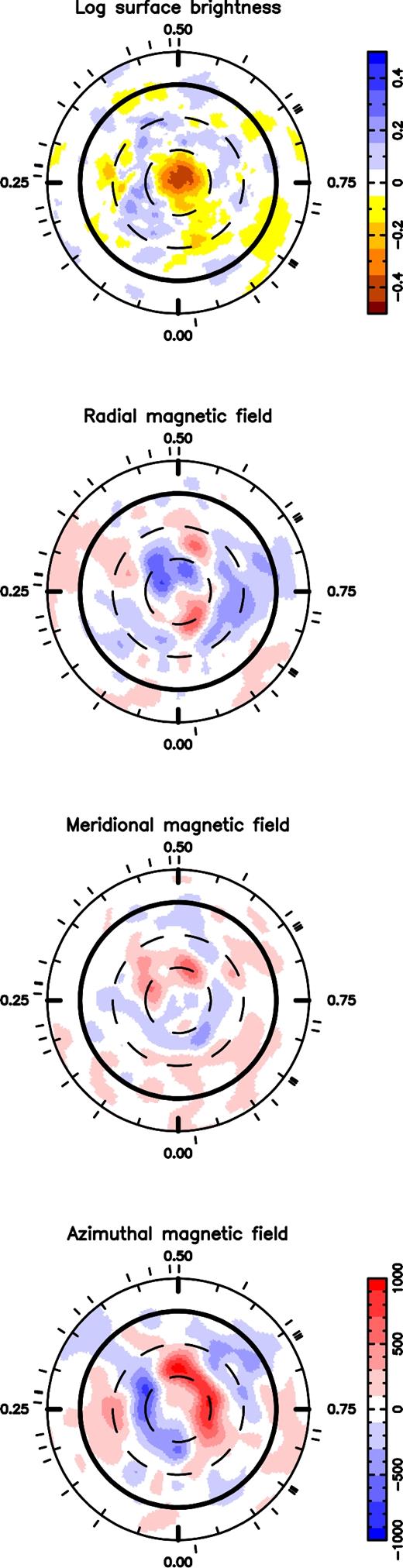
Brightness and magnetic components surface maps when fitting the 2015 November and 2016 January data sets altogether, at rotation cycle 51.

APPENDIX B: ACTIVITY PROXIES

In order to investigate whether the detected periodic RV signal may relate to activity, we plotted periodograms of the longitudinal magnetic field B_ℓ and of the Hα emission equivalent width (Figs B1 and B2, respectively). Peak frequencies for these proxies are located at periods of 0.7145 ± 0.0002 d and 0.7132 ± 0.0001 d, respectively, as well as their aliases. Given the surface differential rotation parameters measured for TAP 26 (see Section 4.2), the values of their respective periods indicate that the longitudinal field traces an average latitude of 46° whereas the bulk of Hα emission comes from a lower average latitude of 27° (see equation 2). As opposed to the raw RVs, the rotation period P_rot has a higher power than its first harmonic P_rot/2 (Fig. 10). No signal is detected at the planet periods found in Section 5.

Figure B1.

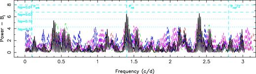
Periodogram of the longitudinal magnetic field. The rotation period at 0.7135 d is represented by a dashed vertical cyan line, as well as its first harmonic and the orbital period at 10.92 d.

Figure B2.

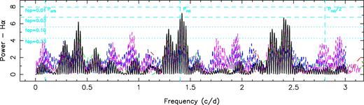
Periodogram of the Hα line equivalent width. The rotation period at 0.7135 d is represented by a dashed vertical cyan line, as well as its first harmonic and the orbital period at 10.92 d.

Plotting phase-folded curves of the longitudinal magnetic field and the Hα emission equivalent width (where the x-axis indicates the rotation phase as defined in equation 1), in Figs B3 and B4, we observe a decrease in the longitudinal magnetic field around phase 0.77 in 2015 November and phase 0.97 in 2016 January, which correspond approximately to the phases where the dipole pole points towards the Earth (0.73 ± 0.03 and 0.85 ± 0.03, respectively), causing B_ℓ to have strong negative values and showing the importance of the dipole in the value of B_ℓ. Similarly, the increase in emission equivalent width of the Hα line between phases 0.6 and 0.9 illustrates the correlation between the lower harmonics of the magnetic field of TAP 26 and this activity proxy.

Figure B3.

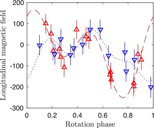
Folded curve of the longitudinal magnetic field against the rotation phase. 2015 November (red upward-pointing triangles) data are fitted with the sum of a sine curve and one harmonic (red dashed line) and 2016 January (blue downward-pointing triangles) data are fitted with the sum of a sine curve and two harmonics (blue dotted line).

Figure B4.

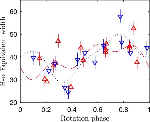
Folded curve of the equivalent width of Hα against the rotation phase. 2015 November (red upward-pointing triangles) and 2016 January (blue downward-pointing triangles) data are fitted with the sum of a sine curve and two harmonics (red dashed line and blue dotted line, respectively).