The masses of retired A stars with asteroseismology: Kepler and K2 observations of exoplanet hosts

Abstract

We investigate the masses of ‘retired A stars’ using asteroseismic detections on seven low-luminosity red-giant and sub-giant stars observed by the NASA Kepler and K2 missions. Our aim is to explore whether masses derived from spectroscopy and isochrone fitting may have been systematically overestimated. Our targets have all previously been subject to long-term radial velocity observations to detect orbiting bodies, and satisfy the criteria used by Johnson et al. to select survey stars which may have had A-type (or early F-type) main-sequence progenitors. The sample actually spans a somewhat wider range in mass, from ≈ 1 M_⊙ up to ≈ 1.7 M_⊙. Whilst for five of the seven stars the reported discovery mass from spectroscopy exceeds the mass estimated using asteroseismology, there is no strong evidence for a significant, systematic bias across the sample. Moreover, comparisons with other masses from the literature show that the absolute scale of any differences is highly sensitive to the chosen reference literature mass, with the scatter between different literature masses significantly larger than reported error bars. We find that any mass difference can be explained through use of different constraints during the recovery process. We also conclude that underestimated uncertainties on the input parameters can significantly bias the recovered stellar masses, which may have contributed to the controversy on the mass scale for retired A stars.

asteroseismology, techniques: photometric, stars: evolution, stars: fundamental parameters

1 INTRODUCTION

Long-term radial velocity surveys have discovered a population of giant planets on ≥300  d orbits around evolved stars that are more massive than the Sun (Johnson et al. 2007a; Bowler et al. 2010; Wittenmyer et al. 2011). These host stars would have been spectral type A on the main sequence. Evolved stars were targeted since A-type stars are hostile to radial velocity observations on the main sequence, due to rapid rotation broadening spectral lines (Johnson et al. 2007a). These stars show a population of planets distinct from the planets discovered via transit surveys, particularly the vast numbers of planets discovered by the NASA Kepler and K2 missions (Borucki et al. 2010; Johnson et al. 2010b; Fressin et al. 2013; Howell et al. 2014). It remains unclear if the different populations observed are a single population observed with strong selection effects, or if the different populations of planets truly indicate separate planet formation mechanisms (Fischer & Valenti 2005; Howard et al. 2010; Becker et al. 2015).

Recently the masses of evolved stars have been brought into question on several grounds (Lloyd 2011; Schlaufman & Winn 2013), with the possibility raised that the masses of evolved hosts have been overestimated when derived from spectroscopic observations. The mass of these stars is typically recovered by interpolating grids of stellar models to the observed T_eff, log g and [Fe/H], and including additional parameters such as luminosity and colours where available (see Johnson et al. 2007a and references therein). These stellar models are then explored in a probabilistic fashion to find the best solution for the fundamental stellar properties (da Silva et al. 2006; Ghezzi & Johnson 2015).

These evolved stars have been termed ‘retired A stars’ in current literature (Johnson et al. 2008; Bowler et al. 2010; Lloyd 2011), since the derived masses for these stars are typically M ≳ 1.6 M_⊙, i.e around the boundary in stellar mass between A- and F-type stars on the main sequence. We follow that convention in this work, but note that the term ‘retired A stars’ can extend to the stellar mass range more typically associated with hot F-type stars on the main sequence (∼1.3–1.6 M_⊙).

To try and resolve the above issues, another analysis method to determine the masses of evolved stars is needed. The high-quality data from the Kepler and K2 missions provide an opportunity to perform asteroseismology (Gilliland et al. 2010; Chaplin et al. 2015) on known evolved exoplanet hosts (Campante et al. 2017). In this paper, we investigate seven stars that have been labelled ‘retired A stars’ in the literature, and use a homogeneous asteroseismic analysis method to provide accurate and precise masses. For the ensemble, we investigate the fundamental stellar properties estimated from different combinations of spectroscopic and asteroseismic parameters. The stellar masses are estimated by fitting grids of stellar models to the observable constraints. With these masses we address any potential systematic bias in the masses of evolved hosts, when the masses are derived from purely spectroscopic parameters. We also investigate potential biases due to the choice of the stellar models used.

The format of the paper is as follows. Section 2 describes how the targets were selected and vetted. Section 3 discusses how the light curves were processed to allow the solar-like oscillations to be detected and how the asteroseismic parameters were extracted from the observations, whilst Section 4 details any previous mass results for each star in turn, and any subtleties required during the extraction of the asteroseismic parameters. The modelling of the stars to estimate the fundamental stellar properties is discussed in Section 5. The final results are in Section 6. In Section 7, we explore in detail potential sources of biases in recovering the fundamental parameters, along with a detailed discussion of potential biases induced in stellar modelling due to differences in constraints and underlying physics.

2 TARGET SELECTION

Targets were selected from cross-referencing the K2 Ecliptic Plane Input Catalog (EPIC) (Huber et al. 2016) and the NASA Exoplanet Archive (Akeson et al. 2013), where only confirmed planets discovered by radial velocity were retained. The resulting list was then cross-checked with the K2FOV tool (Mullally, Barclay & Barentsen 2016) to ensure the stars were observed during the K2 mission. To ensure these hosts were all selected from the correct area of parameter space, it was also checked that they all passed the target selection of Johnson et al. (2006) with 0.5 < M_V < 3.5, 0.55 < B − V < 1.0¹. This produces six stars in Campaigns 1–10 (C1–10).

The light curve for the star identified in C1 was found to be of too low quality to observe stellar oscillations. An additional target was found in C2, through checking targets in K2 guest observer programmes² of bright evolved stars that have been subject to long-term radial velocity observations (Wittenmyer et al. 2011). This star was not identified in the initial selection as it is not a host star but it passes the colour and absolute magnitude selection of Johnson et al. (2006).

HD 212771 was also subject to asteroseismic analysis in Campante et al. (2017) using the same methods presented in Section 5.

In addition the retired A star HD 185351, observed during the nominal Kepler mission, has been added to the sample. This star has already been subject to asteroseismic analysis in Johnson et al. (2014). However it has been added to this sample for reanalysis for completeness.

The seven stars in our ensemble are summarized in Table 1, including which guest observer programme(s) the stars were part of. Before we discuss the previous mass estimates for each star in Section 4, we discuss the data collection and preparation required to extract the asteroseismic parameters from the K2 data.

Table 1.

The seven stars to be investigated in the paper, all have been observed by either the Kepler or K2 mission, and subject to long-term radial velocity observations. The Obs column indicates what observing campaign of K2 the star was observed in (C2–10), or if it was observed in the Kepler mission (KIC). The GO column indicates which K2 guest observer programme(s) the star was part of.

EPIC/KIC	HD	Obs	Mag (V)	RA (h:m:s)	Dec (d:m:s)	GO
203514293	145428	C2a	7.75	16:11:51.250	−25:53:00.86	2025, 2071, 2109
220548055	4313	C8	7.82	00 45 40.359	+07 50 42.07	8031, 8036, 8040, 8063
215745876	181342	C7	7.55	19:21:04.233	−23:37:10.45	7041, 7075, 7084
220222356	5319	C8a	8.05	00:55:01.400	+00:47:22.40	8002, 8036, 8040
8566020	185351	KICa	5.169	19:36:37.975	+44:41:41.77	N/A
205924248	212771	C3a	7.60	22:27:03.071	−17:15:49.16	3025, 3095, 3110
228737206	106270	C10a	7.58	12 13 37.285	−09 30 48.17	10002, 10031, 10040, 10051, 10077

^aObserved in short cadence mode.

3 OBSERVATIONS AND DATA PREPARATION

All targets have been subject to long-term radial velocity programmes attempting to detect the periodic stellar radial velocity shifts induced by orbiting planets. However, for the purposes of asteroseismology high-quality, uninterrupted photometry is required. This was achieved during the Kepler and K2 missions.

The light curves for the K2 targets were produced from the target pixel files using the K2P² pipeline (Lund et al. 2015), and then subsequently corrected using the KASOC filter (Handberg & Lund 2014). Table 1 indicates if the stars were observed at a cadence of ∼1 min (short cadence) or ∼30 min (long cadence).

The evolved stars in this paper are expected to exhibit solar-like oscillations, with near surface convection driving global oscillation modes (p and g modes) inside the star. Such oscillations have been observed in thousands of red giants by the Kepler and K2 missions (Huber et al. 2010; Hekker et al. 2011; Stello et al. 2013, 2015). Fig. 1 shows all the power spectra produced from the corrected light curves for the ensemble. In all targets there are clear signatures of solar-like oscillations, above the granulation background.

Figure 1.

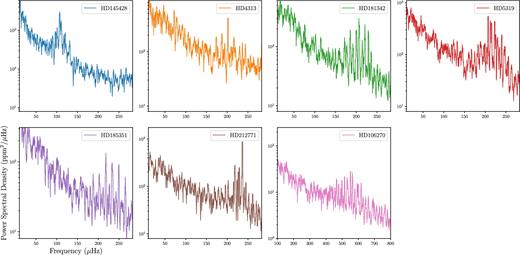
The power spectra for each star in our sample, smoothed by a 2μHz uniform filter (4μHz in the case of HD 106270), from which we extract the asteroseismic parameters. The stellar oscillations are clearly visible above the granulation background. Note the change in scale for the Campaign 10 star, HD 106270. The stars are presented in order of increasing ν_max.

Here, we make use of the so-called global asteroseismic parameters; ν_max, the frequency of maximum power and Δν, the average large frequency separation, defined as the average frequency spacing between acoustic oscillation modes of the same angular degree l and consecutive radial order n. In Table 1 the values are ordered by increasing ν_max, as are in Tables 2 and 4.

Table 2.

The final asteroseismic and spectroscopic inputs and output stellar parameters from the modelling. The effective temperature and metallicity used for each source are taken as matched pairs from the same source.

EPIC/KIC	HD	Δν (μHz)	νmax (μHz)	Teff (K)	[Fe/H]		Mass (M⊙)	Radius (R⊙)	Age (Gyr)
203514293*	145428	10.1 ± 0.3	107 ± 2	4818 ± 100a	−0.32 ± 0.12a		|$0.99^{+0.10}_{-0.07}$|	|$5.51^{+0.26}_{-0.19}$|	|$9.03^{+2.79}_{-2.72}$|
220548055	4313	14.1 ± 0.3	201 ± 8	4966 ± 70b	0.05 ± 0.1b		|$1.61^{+0.13}_{-0.12}$|	|$5.15^{+0.18}_{-0.17}$|	|$2.03^{+0.64}_{-0.45}$|
215745876	181342	14.4 ± 0.3	209 ± 6	4965 ± 80b	0.15 ± 0.1b		|$1.73^{+0.18}_{-0.13}$|	|$5.23^{+0.25}_{-0.18}$|	|$1.69^{+0.47}_{-0.41}$|
220222356	5319	15.9 ± 0.5	216 ± 3	4869 ± 80b	0.02 ± 0.1b		|$1.25^{+0.11}_{-0.10}$|	|$4.37^{+0.17}_{0.17}$|	|$5.04^{+1.78}_{-1.30}$|
8566020*	185351	15.6 ± 0.2	230 ± 7	5035 ± 80c	0.1 ± 0.1c		|$1.77^{+0.08}_{-0.08}$|	|$5.02^{+0.12}_{-0.11}$|	|$1.51^{+0.17}_{-0.14}$|
205924248	212771	16.5 ± 0.3	231 ± 3	5065 ± 95d	−0.1 ± 0.12d		|$1.46^{+0.09}_{-0.09}$|	|$4.53^{+0.13}_{-0.13}$|	|$2.46^{+0.67}_{-0.50}$|
228737206*	106270	32.6 ± 0.5	539 ± 13	5601 ± 65b	0.06 ± 0.1b		|$1.52^{+0.04}_{-0.05}$|	|$2.95^{+0.04}_{-0.04}$|	|$2.26^{+0.06}_{-0.05}$|
param uses [M/H], which we take to equal [Fe/H] for all stars.
Quoted errors on mass, radius and age are the 68 per cent credible interval from param.

*Gaia TGAS parallaxes were unavailable, or believed unreliable (see Section 5.2), and so the Hipparcos parallax is used instead in the construction of the stellar luminosity.

^aWittenmyer et al. (2016).

^bMortier et al. (2013).

^cGhezzi et al. (2015).

^dCampante et al. (2017).

These seismic parameters were extracted from each power spectrum using a variety of well established and thoroughly tested automated methods (Huber et al. 2009; Verner et al. 2011; Davies & Miglio 2016; Lund et al. 2016). The values used in subsequent analysis are those returned by the method described in Huber et al. (2009). Since multiple pipelines were used to extract the parameters, the uncertainties used in the modelling are the formal errors returned by the Huber et al. (2009) pipeline with the standard deviation of the errors returned from the other methods added in quadrature. This additional uncertainty should account for any unknown systematics in each of the recovery methods. When compared to the seismic values returned by the Huber et al. (2009) pipeline, none of the methods differ by more than 1.3σ in Δν, and less than 1σ in ν_max. Line-of-sight velocity effects are negligible and do not affect the seismic results (Davies et al. 2014).

An additional asteroseismic parameter, where available, is the average g-mode period spacing, accessed through l = 1 ‘mixed’ modes (Beck et al. 2011; Mosser et al. 2011). Mixed modes can be highly informative in constraining stellar models and the core conditions of evolved stars (Bedding et al. 2011; Lagarde et al. 2016). Unfortunately due to the shorter length of K2 data sets and hence limited frequency resolution, the period spacing is inaccessible for the six K2 targets in our ensemble.

4 STAR-BY-STAR VETTING

In this section, we discuss any individual peculiarities of each star separately. Particular focus is placed on HD 185351, which has been subjected to a suite of investigations throughout and after the nominal Kepler mission (Johnson et al. 2014; Ghezzi, do Nascimento & Johnson 2015; Hjørringgaard et al. 2017). All available literature masses for the stars in our ensemble are summarized in Table A1. The final seismic and spectroscopic values used in the stellar modelling are summarized in Table 2.

4.1 HD 145428

The most evolved star in our sample, HD 145428, it is not currently known to host planets, but was a target of the Pan-Pacific Planet Search (PPPS; Wittenmyer et al. 2011) conducted on the Southern sky from the 3.9 m Anglo–Australian Telescope. Here, we use updated spectroscopic parameters from Wittenmyer et al. (2016). The target selection for the PPPS is very similar to the target selection used in the Lick & Keck Doppler survey (Johnson et al. 2006, 2007a,b). This star passes the absolute magnitude selection criteria of Johnson et al. (2006), however B − V = 1.02 for this star is slightly over the B − V ≤ 1 selection cut. It was decided to retain this star in the sample despite this. Whilst most of the stars in our sample have multiple mass values quoted in the literature, this star appears to have been subject to minimal study, limiting the scope of comparison between asteroseismic and spectroscopic mass estimates.

4.2 HD 4313

HD 4313, an exoplanet host announced in Johnson et al. (2010b) shows evidence for suppressed l = 1 modes, first identified as a feature in red giant power spectra in Mosser et al. (2012). The cause for such suppression is currently under discussion (see Fuller et al. 2015; Mosser et al. 2017; Stello et al. 2016), though in this case we assume that it is not a planet-based interaction, since the planet HD 4313b has an orbital period of approximately 1 yr. The limited number of observable oscillation modes also has an impact on the precision of the seismic values, as reflected in the uncertainty on ν_max in Table 2.

4.3 HD 181342

HD 181342, an exoplanet host reported in Johnson et al. (2010a), has the largest spread in reported masses, with estimates from 1.20–1.89 M_⊙ (Huber et al. 2016; Jones et al. 2016).

4.4 HD 5319

HD 5319, is the only known multiple planet system in our sample. Both discovery papers list stellar masses in excess of M > 1.5 M_⊙ (Robinson et al. 2007; Giguere et al. 2015).

4.5 HD 185351

HD 185351 (KIC 8566020), one of the brightest stars in the Kepler field, has been monitored as part of a Doppler velocity survey to detect exoplanets (Johnson et al. 2006), though no planet has been found. Additionally in Johnson et al. (2014) (hereafter Johnson et al. 2014) the star was studied using asteroseismology, comparing the stellar properties determined from various complementary methods, including an interferometric determination of the stellar radius. Several mass values are given, in the range 1.6–1.99 M_⊙. As mentioned above, the observed period spacing between mixed modes can be an important constraint on core properties and so on global stellar properties. In Johnson et al. (2014), a period spacing ΔΠ = 104.7 ± 0.2 s⁻¹ is given. Since we wish to perform a homogeneous analysis for the ensemble, we do not include a period spacing for the star during the recovery of the stellar properties in Section 5.

4.6 HD 212771

This is an exoplanet host detected in Johnson et al. (2010a). The mass reported in the discovery paper, M = 1.15 M_⊙, is consistent with a retired F- or G-type star. However, the recent work by Campante et al. (2017) provides an asteroseismic mass of M = 1.45 M_⊙, promoting this star to a retired A star. This mass was recovered using the same methodology as used in this work. We present an updated mass in this work, though the shift is negligible.

4.7 HD 106270

The final star in our ensemble, this exoplanet host reported in Johnson et al. (2011) is significantly less evolved than the rest of the ensemble.

5 MODELLING

5.1 Stellar models

With the asteroseismic parameters determined for each star, the modelling of the ensemble to extract fundamental stellar properties could now take place. We use mesa models (Paxton et al. 2011, 2013) in conjunction with the Bayesian code param (da Silva et al. 2006; Rodrigues et al. 2017). A summary of our selected ‘benchmark’ options is as follows.

• Heavy element partitioning from Grevesse & Noels (1993).

• OPAL equation of state (Rogers & Nayfonov 2002) along with OPAL opacities (Iglesias & Rogers 1996), with complementary values at low temperatures from Ferguson et al. (2005).

• Nuclear reaction rates from NACRE (Angulo et al. 1999).

• The atmosphere model is taken according to Krishna Swamy (1966).

• The mixing length theory was used to describe convection (a solar-calibrated parameter α_MLT = 1.9657 was adopted).

• Convective overshooting on the main sequence is set to α_ov = 0.2H_p, with H_p the pressure scaleheight at the border of the convective core (more on this in Section 7.2). Overshooting was applied according to the Maeder (1975) step function scheme.

• No rotational mixing or diffusion is included.

• When using asteroseismic constraints, the large frequency separation Δν within the mesa model is calculated from theoretical radial mode frequencies, rather than based on asteroseismic scaling relations.

Below, we discuss the additional inputs required for the modelling, such as T_eff, [Fe/H] and luminosity.

In Section 7.2, we test the robustness of the asteroseismic masses by varying the underlying model physics, and explore the effects of unaccounted for biases in the stellar observations.

5.2 Additional modelling inputs

In addition to the asteroseismic parameters, temperature and metallicity values are needed for each star. Since multiple literature values exist for the chosen targets, we had to choose a source for each. To ensure the values are self-consistent, when a literature value was chosen for temperature, we took the stellar metallicity from the same source i.e. matched pairs of temperature and metallicity. To account for unknown systematics additional uncertainties of 59K and 0.062 dex were added in quadrature (Torres et al. 2012), to the chosen literature values. Several of the stars have smaller reported [FeH] error bars than the systematic correction of Torres et al. (2012), for these stars an error bar of 0.1 dex was adopted.

The stellar luminosity also provides a strong constraint on the modelling. The luminosity may be estimated as follows (e.g. see Pijpers 2003):

\begin{eqnarray} \log _{10} \frac{L}{{\rm L}_{{\odot }}} &=& 4.0+ 0.4 M_{{\textrm{bol}},{\odot }} -2.0 \log _{10} {\pi [{\textrm{mas}]}} \nonumber\\ &&- 0.4(V-A_V + BC(V)). \end{eqnarray}

(1)

Johnson V magnitudes and uncertainties were taken from the EPIC (Huber et al. 2016), the solar bolometric magnitude M_bol⊙ = 4.73 is taken from Torres (2010), from which we also take the polynomial expression for the bolometric correction³BC(V). Finally, the extinction A_V is calculated using MWDUST (Bovy et al. 2016)⁴, using the 3D dust maps from Green et al. (2015).

5.3 Parallaxes

Parallaxes π were taken from Hipparcos (van Leeuwen 2007) and the recent Tycho-Gaia Astrometric Solution (TGAS) data release, part of the Gaia Data Release 1 (Lindegren et al. 2016). The Gaia parallax is generally preferred. HD 185351 and HD 106270 are both missing Gaia TGAS parallaxes due to their bright apparent magnitudes, with Gaia DR1 missing many stars with Gaia magnitude G ≤ 7. For stars with a TGAS parallax, an additional uncertainty of 0.3 mas has been added to the formal parallax uncertainty as suggested by Lindegren et al. (2016). Campante et al. (2017) previously found that the Hipparcos solution for the distance to HD 212771 is in tension with the asteroseismic solution, whilst the Gaia solution is entirely consistent.

Conversely, the luminosity constructed using equation (1) for HD 145428 was severely discrepant due to the large difference between the Gaia and Hipparcos parallaxes (5.39 ± 0.73 mas and 7.62 ± 0.81 mas, respectively). When the final stellar radius from the modelling is used along with the input temperature, the constructed luminosity is found to be consistent with the Hipparcos luminosity, but not with the Gaia luminosity. As such the Gaia luminosity was also ignored in this case, and all modelling results for this star are reported using a Hipparcos parallax based luminosity. There has been discussion in the literature of possible offsets in the Gaia parallaxes when compared to distances derived from eclipsing binaries (Stassun & Torres 2016) and asteroseismology (De Ridder et al. 2016; Davies et al. 2017; Huber et al. 2017).

6 RESULTS

Table 2 summarizes the asteroseismic and spectroscopic inputs used in the analysis and the estimated stellar properties returned by param for our benchmark set of chosen input physics. Additional modelling using different constraints and model grids is discussed in Section 7.

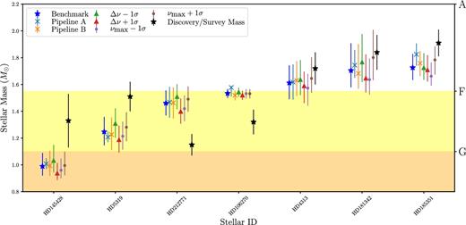
With the results from param we can now compare the stellar masses derived from asteroseismology with the other literature values. Fig. 2 shows the different mass estimates from available literature sources (see Table A1), with the masses reported in the planet discovery or survey paper, our primary comparison mass, as black stars. The asteroseismic masses (red diamonds) are shown alongside other literature values (points).

Figure 2.

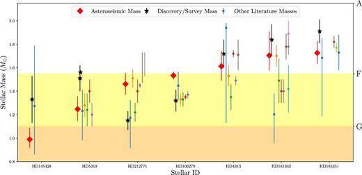
Mass versus ID, the horizontal bars indicate approximate spectral type on the main sequence, (AFG corresponding to white, yellow and orange, respectively). Black stars indicate the mass of the star as reported in the planet survey or planet detection paper. Red diamonds indicate the param stellar mass from Table 2, whilst dots indicate other literature values for each star. As can be seen for several of the stars (HD 5319, HD 145428, HD 181342 and HD 212771), the different mass estimates can cover the entire spectral range of G to A type.

For the survey mass of HD 185351, no error was provided with the value in Bowler et al. (2010). We adopt the σ_M = 0.07 from Johnson et al. (2014), who in their interpolation of spectroscopic parameters on to isochrones recovered a similar mass to Bowler et al. (2010).

The survey mass of HD 145428 in Wittenmyer et al. (2016) also has no reported formal error bar, although the work quotes ‘typical uncertainties 0.15–0.25 M_⊙’. As such we take 0.2 M_⊙ as the uncertainty.

To investigate the mass discrepancies between different methods, we plot the difference between the literature values and the asteroseismic masses, versus stellar ID, after arranging stars in the sample in terms of increasing stellar mass, in Fig. 3.

Figure 3.

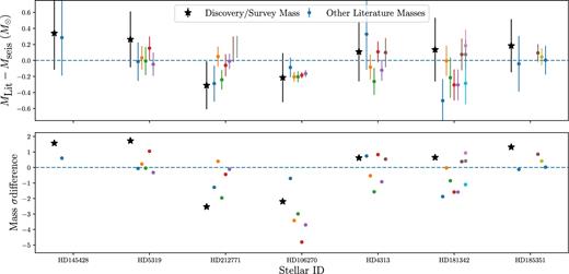
Difference between literature and asteroseismic masses, against stellar ID, arranged by increasing stellar mass. Negative values indicate the asteroseismic mass is greater than the literature mass. Again we plot the mass difference with the planet survey mass as a black star. The error bars are the mean seismic error added in quadrature to the literature error bar. The lower panel shows the σ difference between the seismic mass and literature mass, where the errors have been added in quadrature.

A striking feature of Fig. 2 is the size of the error bars on each literature mass value, compared to the scatter on the mass values. Several stars have literature mass values with reported error bars of ≈0.1 M_⊙, i.e. quite precise estimates, but with individual mass estimates scattered across a ≥0.5 M_⊙ region. HD 4313, HD 181342 and HD 212771 all show this level of scatter on literature mass values.

Fig. 3 shows the difference in mass estimates, taking the asteroseismic mass as the reference value. Values below zero indicate that the literature mass is lower than the seismic mass. The lower panel in the figure shows the difference in standard deviations between the mass estimates, where the literature mass and asteroseismic mass have had their errors added in quadrature. As can be seen, five of the seven stars display asteroseismic masses below the masses reported in the planet discovery/survey paper, however at a ≤2σ level. HD 212771 and HD 106270 show the opposite behaviour. We caution against taking this difference in asteroseismic masses to be evidence for a systematic shift in stellar mass, due to the small sample size. The average mass offset of the seismic to survey mass is ΔM = 0.07 ± 0.09 M_⊙.

A simple Monte Carlo test was performed to investigate the probability that five out of seven proxy spectroscopic masses would exceed five proxy seismic masses for our quoted uncertainties, assuming both of the masses are drawn from normal distributions with a mean of the seismic mass. We found that for a million independent realisations, 16 per cent of the time five of the proxy spectroscopic masses exceed the proxy seismic masses. As such, we see that there is no clear bias between asteroseismic masses and other methods. If we instead derive model independent asteroseismic masses – using the well-known asteroseismic scaling relations (e.g. see discussion in Chaplin & Miglio 2013) – we find no difference in this result or other results in the paper.

In Section 1, we discuss that the term ‘retired A star’ can be used to describe masses associated with hot F stars as well as A-type stars. However, if we consider the masses in Table 2, neither HD 145428 (0.99 M_⊙) or HD 5319 (1.25 M_⊙) can be categorized as such. If we therefore discard these stars, then only three of the five remaining stars have seismic masses below the survey mass, with the average offset ΔM = 0.02 ± 0.09 M_⊙.

Since the survey masses are a heterogeneous sample of masses, we also compare the seismic masses to several other literature sources (see Table A1). Unfortunately, no single source has masses for all of our stars, and so each homogeneous set of reference masses is a subset of the ensemble. The average ratios are shown in Table 3. This choice of reference literature mass has a strong impact on the size (and sign) of any observed mass offset. Fig. A1 shows the distribution of mass ratios for each literature reference mass.

Table 3.

The mean fractional offset of various sets of homogeneous literature mass sources compared to the seismic mass.

Reference	N Stars	Offset
Discovery/Survey	7	1.07 ± 0.07
Mortier et al. (2013)a	5	0.97 ± 0.03
Mortier et al. (2013)b	5	0.88 ± 0.03
Jofré et al. (2015)	4	1.06 ± 0.01
Bonfanti et al. (2015)	5	0.97 ± 0.05
Bonfanti, Ortolani & Nascimbeni (2016)	5	0.91 ± 0.03

^aTsantaki et al. (2013) line list.

^bHekker & Meléndez (2007) line list.

7 DISCUSSION

In order to investigate the robustness of recovering single star masses from stellar models, with or without the inclusion of asteroseismic parameters, we now explore the potential biases from the use of different stellar models, inputs and error bars on the recovered stellar mass.

7.1 Use of different constraints

Throughout this work we have considered the asteroseismic mass to be the mass returned by param using all available asteroseismic, spectroscopic and parallax/luminosity constraints. To see how much the non-asteroseismic constraints are influencing the final stellar mass, we also ran param using only T_eff, [Fe/H] and luminosity, i.e. without seismology. This was done in an effort to emulate the procedure used in Johnson et al. (2010a), using the same constraints but different model grids. Ghezzi & Johnson (2015) previously found that stellar masses can be recovered to good precision using parsec models and only spectroscopic constraints. The different mass results for each star are shown in Fig. 4 and are summarized in Table 4.

Figure 4.

All the different mass estimates using mesa, parsec and mist grids (labelled isoclassify), the mesa and parsec grids were ran with and without seismic constraints. Blue stars are the results from Table 2. Crosses are masses with seismic and luminosity constraints, points are non-seismic constraints only (T_eff, [FeH], L). The overshooting parameter used in the models is indicated by the ‘ov0*’ label. parsec tracks show significant shifts, as do non-seismic results at higher masses. Subgiant HD 106270 shows unique behaviour most likely due to being a subgiant, rather than red giant.

Table 4.

Comparing stellar masses estimated using different physics and constraints. All in Solar masses  M_⊙.

EPIC/KIC	HD	mesa without seismologya	mesab (αov = 0.0Hp)	parsecc	isoclassifyd
203514293	145428	|$1.05^{+0.23}_{-0.12}$|	|$0.97^{+0.09}_{-0.06}$|	|$0.99^{+0.10}_{-0.07}$|	|$1.17^{+0.14}_{-0.12}$|
220548055	4313	|$1.56^{+0.14}_{-0.16}$|	|$1.67^{+0.14}_{-0.14}$|	|$1.55^{+0.15}_{-0.16}$|	|$1.67^{+0.18}_{-0.15}$|
215745876	181342	|$1.50^{+0.19}_{-0.23}$|	|$1.75^{+0.14}_{-0.13}$|	|$1.74^{+0.14}_{-0.15}$|	|$1.82^{+0.20}_{-0.20}$|
220222356	5319	|$1.22^{+0.19}_{-0.17}$|	|$1.24^{+0.11}_{-0.10}$|	|$1.23^{+0.09}_{-0.10}$|	|$1.35^{+0.11}_{-0.11}$|
8566020	185351	|$1.50^{+0.17}_{-0.22}$|	|$1.74^{0.08}_{-0.08}$|	|$1.80^{+0.09}_{-0.09}$|	|$1.83^{+0.12}_{-0.10}$|
205924248	212771	|$1.41^{+0.17}_{-0.21}$|	|$1.45^{+0.10}_{-0.10}$|	|$1.38^{+0.10}_{-0.07}$|	|$1.47^{+0.09}_{-0.08}$|
228737206	106270	|$1.37^{+0.07}_{-0.07}$|	|$1.56^{+0.04}_{-0.04}$|	|$1.42^{+0.02}_{-0.02}$|	|$1.41^{+0.03}_{-0.06}$|

^amesa models (α_ov = 0.2H_p) with [FeH], T_eff and luminosity.

^bmesa models ran with α_ov = 0.0H_p.

^cparsec models.

^dmist models ran with isoclassify.

Before we discuss the results, we introduce the additional modelling performed using different underlying physics in the stellar models chosen.

7.2 Use of different model grids

To test the sensitivity of the derived stellar masses to the models used, extra grids of mesa models were created. The models described in Section 5 include a convective-overshooting parameter α_ov during the main sequence, which changes the size of the helium core during the red giant branch phase. This was set to α_ov = 0.2H_p where H_p is the pressure scaleheight. To investigate the impact of changing the underlying model physics on the final stellar mass result, new grids of models with the overshooting parameter adjusted to α_ov = 0.1H_p or 0 were generated and param run using these new models. This parameter was chosen to be varied, since stars in the mass range of retired A stars have convective core during the main sequence. Two further grids of models were used. First, we adopted parsec stellar models, which parametrize overshooting as a mass-dependent parameter (see Bressan et al. 2012; Bossini et al. 2015). Secondly, a grid of mist (mesa Isochrones and Stellar Tracks; Choi et al. 2016) models was used in conjunction with the code isoclassify.⁵

Isolating any stellar mass difference between mesa and parsec to a single parameter is not possible, since multiple model parameters are different between the models. Additionally there are multiple differences between the mesa tracks used in Section 5 and the mist tracks. The use of these different tracks here is to explore overall mass differences between the different grids and not to define the precise cause of such a difference.

If we consider first the lower mass stars (HD 5319, HD 145428 and HD 212771), there is no clear trend with overshooting nor does the inclusion of seismology produce a noticeable shift in mass, with the exception of the parsec tracks. The inclusion of luminosity alongside seismic constraints provides the smallest uncertainties.

For the higher mass stars (HD 4313, HD 181342 and HD 185351), there is a clear trend in increasing mass with decreasing overshooting parameter. The recovered masses using seismic constraints are also in general above the mass estimates without seismic constraints. Whilst for HD 4313 the shift in mass is fairly minor, for HD 181342 and HD 185351 the mass offset is ΔM ∼ 0.2 M_⊙. The greatest disparity is between parsec results with and without seismic constraints. Again we note that for five of the seven stars in the ensemble, all of the recovered mass estimates are below the masses reported in the planet discovery papers.

Finally, we look at the subgiant HD 106270. There appears to be no strong mass-overshooting parameter dependence; however, the mesa models produce significantly different masses to the parsec and mist models which should be investigated more closely. Additionally, the mass estimates recovered from the mesa models without seismic constraints are significantly lower with ΔM ∼ 0.2 M_⊙.

When we consider the masses returned without the use of the seismology (blue points in Fig. 4) emulating Johnson et al. (2010a), using the same underlying models that were used with the seismic constraints in Section 5, we fail to recover the same mass as is reported in the discovery paper in most cases. This disparity is presumably due to differences in the underlying stellar models.

When comparing the mist masses (purple crosses) to the benchmark seismic masses (blue stars), the mist results typically recover a higher mass. If we include HD 106270, for which the mist mass is ∼0.1 M_⊙ lower than the benchmark mass, then the average mass offset of the mist masses is ΔM = 0.03 ± 0.06 M_⊙. However if we remove HD 106270, the mist average mass shift is ΔM = 0.05 ± 0.04 M_⊙.

7.3 Potential biases in spectroscopic parameters

An additional discrepancy to highlight is that not only are the final mass values derived from spectroscopic parameters in disagreement with each other, possibly caused by different physics in the models used in each paper during the recovery of the stellar mass, but also the underlying spectroscopic values (T_eff, log g and [FeH]) can be discrepant at a significant level. Fig. 5 highlights this problem. For two of the stars in the sample, HD 106270 and HD 181342, literature T_eff and log g values are plotted over a grid of mesa tracks, using the same physics as in Section 5. In particular, HD 106270 highlights that reported spectroscopic values may be highly precise, but show significant disagreement with other literature values (see Blanco-Cuaresma et al. 2016 for more discussion on the impact of different spectroscopic pipelines and assumed atmospheric physics on derived parameters). The reported values are highly scattered across the subgiant branch in the Kiel diagram in Fig. 5. HD 181342, shown in black, highlights the additional problem with targeting red giant branch stars for planet surveys. As the star evolves off the subgiant branch, and begins the ascent of the giant branch, the stellar evolutionary tracks across a wide range of masses converge into a narrow region of parameter space, with tracks of different mass and metallicity crossing. In the case of HD 181342, taking only the [FeH]=0.0 tracks, masses from 1.2–1.8 M_⊙ are crossed.

Figure 5.

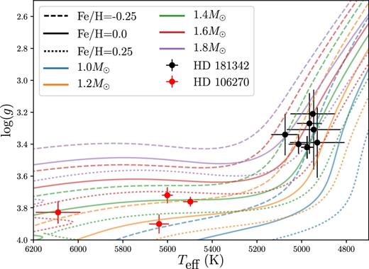
Literature spectroscopic parameters for two of the stars in the sample, showing multiple stellar tracks crossed within the uncertainty region. HD 106270 (red) shows that whilst highly precise spectroscopic values are reported in the literature, this limits the parameter space that isochrone fitting can explore, which can lead to disagreement in recovered masses at a significant level. HD 181342 near the base of the red giant branch shows the convergence of the stellar tracks in that region, increasing the difficulty of recovering the stellar parameters.

In this highly degenerate parameter space, it is naturally difficult to search for and isolate the true stellar mass, requiring highly precise and accurate temperatures to help alleviate the degeneracy. It is in this area that the benefits of asteroseismology become clear, as the additional constraint, provided by the asteroseismic observations allow us to break the degeneracy between the spectroscopic parameters to recover a better estimate of the stellar mass.

Whilst the temperature and metallicity uncertainties presented in Table 1 are around 0.1 dex and ∼80 K, respectively, several of the planet discovery papers for the stars in the ensemble present much smaller uncertainties, e.g. HD 4313, HD 181342 and HD 212771 all presented in Johnson et al. (2010a) have reported errors σ_[FeH] = 0.03dex, σ_Teff = 44K and σ_L = 0.5L_⊙, as does HD 106270 in Johnson et al. (2011). Giguere et al. (2015) quote the same σ_[FeH] and σ_Teff for HD 5319. These spectroscopic parameters and uncertainties were recovered using the package Spectroscopy Made Easy (SME, Valenti & Piskunov 1996).

To explore what impact such tight error bars might have on inferred stellar masses, param was run once more, using the mesa models with overshooting set to α_ov = 0.2H_p (i.e. identical physics and constraints to the masses in Table 2), with the inclusion of the asteroseismic constraints in the fitting. The one change here was a systematic reduction of the error bars on [Fe/H], T_eff and L. In theory, since the same input values and physics are being used, the same values for the stellar mass should be recovered; however, this is not what we find. We have effectively shrunk the available parameter space for param to explore. This parameter space is smaller since the error bars on the input parameters define the width of prior used in the Bayesian methodology. With smaller uncertainties the prior is narrower, and so influences the final results more strongly if the underlying value lies away from the mean of the prior (see da Silva et al. 2006 for more details). To investigate how strongly the seismic values were influencing the recovered parameters, we also ran param using the smaller error bars, without seismic constraints being used, and these results are shown as orange points in Fig. 6. The blue points in Fig. 6 are the results from param using the reduced uncertainties, but including seismic constraints. These mass estimates should agree with the blue stars (the benchmark asteroseismic mass from Table 2) given the same underlying physics and physical parameters. The only change is a reduction in the size of the error bars on temperature, metallicity and luminosity. What we instead see are significant departures from parity, with generally increasing disagreement as a function of increasing mass (though HD 185351 is an exception). This suggests that potentially inaccurate effective temperatures quoted at high precision can prevent the recovery of the true stellar mass. The orange points on Fig. 6 are the results of just using the non-seismic constraints with the deflated error bars discussed above. The recovered mass should be the same as the blue points in Fig. 4 (see Table 4 for masses). Instead we see an average offset of ΔM ∼ 0.1 M_⊙ below the mass in Fig. 4. This is most likely due to the limited parameter space preventing a full exploration of solutions.

Figure 6.

Investigating the effect of biases in the spectroscopic parameters, and underestimated error bars. Black stars are the discovery masses, blue stars are the benchmark asteroseismic masses in Table 2. Blue and orange dots are the same inputs as Table 2 with deflated errors to σ_[FeH] = 0.03dex, σ_Teff = 44K and σ_L = 0.5L_⊙, with and without seismic constraint, respectively. Remaining markers are the inclusion of 1σ biases in T_eff (triangles) and [FeH] (crosses), using the error values in Table 2.

As further tests of the impact of bias in the spectroscopic parameters, param was also run using only the spectroscopic parameters, with artificial biases of 1σ included on T_eff and [FeH]. As Fig. 6 shows, the inclusion of 1σ shifts in T_eff (triangles) or [FeH] (crosses) induces shifts of ∼0.2 M_⊙ in stellar mass for the giant stars.

The subgiant, HD 106270, shows quite separate behaviour and appears more resistant to biases, though it does display a strong disparity in stellar mass estimates with or without asteroseismic constraints. This may be due to the wider separation between tracks of different mass and metallicity at this point in the HR diagram (as seen in Fig. 5). Additionally, since most of the evolution is ‘sideways’ on the subgiant branch, as the star retains a similar luminosity across a range of temperatures, a single mass track can recover the observed spectroscopic parameters (and luminosity) with an adjustment in stellar age.

One potential issue that has not yet been addressed is the systematic offset in log g between seismology and spectroscopy. We compared the log_seisg recovered with the benchmark seismic mass, to the log_specg reported in the literature source from which we take the T_eff and [FeH]. We find the spectroscopic gravities to be overestimated by an average of 0.1 dex. Since the spectroscopic parameters are correlated, this may have introduced biases in the temperature and metallicity we have used in the modelling. To test the impact of any bias, we correct the T_eff and [FeH] by ΔT_eff = 500Δlog g[dex], and Δ[FeH] = 0.3Δlog g[dex] (Huber et al. 2013, see Fig. 2 and surrounding text therein). param was re-run using the mesa models described in Section 5, with the inclusion of the seismic parameters. The mean shift in mass with respect to the benchmark seismic mass was ΔM = −0.0097 ± 0.010 M_⊙. As such, we do not see any evidence for a significant shift in the estimated masses.

7.4 Potential biases in asteroseismic parameters

To ensure a thorough test of potential biases, the input ν_max, Δν values were also separately perturbed by 1σ and param was re-run. We note that in Table 2 both seismic parameters are given to a similar level of precision as the temperatures (average precision on ν_max = 2.4 per cent, Δν = 2.2 per cent and T_eff = 1.6 per cent). Each 1σ perturbation produced an mean absolute shift in mass of ≲0.04 ± 0.009 M_⊙. These mass shifts are approximately five times smaller than those given by the 1σ perturbations to the spectroscopic parameters.

In Section 3, we added additional uncertainties to the error bars on the seismic quantities returned by the Huber et al. (2009) pipeline to account for scatter between pipelines. Here, for completeness, we also tested using as inputs the seismic parameters and formal uncertainties from the other two pipelines. Again, we found very small changes in mass (at the level of or smaller than the uncertainties on the data). These results are shown in Fig. 7.

Figure 7.

Investigating the effect of biases in the seismic parameters, and potentially underestimated error bars. Black stars are the discovery masses, blue stars are the benchmark asteroseismic masses in Table 2. Pipeline A and B (crosses) are two of the pipelines used to recover the asteroseismic parameters. Triangles are the Δν values in Table 2 perturbed by 1σ. Dots are the ν_max values in Table 2 perturbed by 1σ.

8 CONCLUSIONS

This work has explored the masses of so-called retired A Stars and the impact of different stellar models and the individual constraints used on the recovery of the stellar mass for single stars. In our ensemble of seven stars, we find for five of the stars a mild shift to lower mass, when the asteroseismic mass is compared to the mass reported in the planet discovery paper. This mass shift is not significant. Additionally, the scale and sign of this mass offset is highly dependent on the chosen reference masses, as different literature masses for the ensemble cover the mass range 1–2 M_⊙, with optimistic error bars on literature masses resulting in significant offsets between different reference masses. We note that Stello et al. (in preparation) find a similar, non-significant offset for stars of comparable mass to ours (from analysis of ground-based asteroseismic data collected on a sample of very bright A-type hosts), with evidence for an offset in a higher range of mass not explored in our sample. Stello et al. (in preparation) also find that the scatter on the literature values is of comparable size to the observed mass offset.

We also find that the mass difference can be explained through use of different constraints during the recovery process. We also find that ≈0.2 M_⊙ shifts in mass can be produced by only 1σ changes in temperature or metallicity, if only using spectroscopic and luminosity constraints. Additionally we find that even with the inclusion of asteroseismology, potentially inaccurate effective temperatures quoted with high precision makes the recovery of the true mass impossible. To solve this effective spectroscopic temperatures need calibrating to results from interferometry. Finally, we find that the use of optimistic uncertainties on input parameters has the potential to significantly bias the recovered stellar masses. The consequence of such an action would be to bias inferred planet occurrence rates, an argument broadly in agreement with the space-motion based argument of Schlaufman & Winn (2013), i.e. that the masses of evolved exoplanet hosts must be overestimated to explain the observed space motions of the same stars.

Additionally an exploration of differences in recovered mass using different stellar grids needs to be applied to a far larger number of stars, along with a full exploration of which underlying physical parameters are the cause of systematic shifts in mass. This will be the product of future work. Asteroseismic observations of more evolved exoplanet hosts will also be provided by data from later K2 campaigns and from the upcoming NASA TESS Mission (e.g. see Campante et al. 2016).

Acknowledgements

We would like to thank D. Stello for helpful discussion. We also wish to thank the anonymous referee for helpful comments. This paper includes data collected by the Kepler and K2 missions. We acknowledge the support of the UK Science and Technology Facilities Council (STFC). Funding for the Stellar Astrophysics Centre is provided by the Danish National Research Foundation (Grant DNRF106). MNL acknowledges the support of The Danish Council for Independent Research – Natural Science (Grant DFF-4181-00415). This research has made use of the SIMBAD data base, operated at CDS, Strasbourg, France.

1

The selection function also contains an apparent magnitude cut of V ≤ 7.6. We ignore this cut, as this was imposed originally to limit the required exposure time for the stellar spectra and does not influence the fundamental properties of the stars themselves.

2

Targets found using GO programmes and targets listed here, https://keplerscience.arc.nasa.gov/k2-approved-programs.html

3

The polynomial bolometric corrections presented in Torres (2010) are reprints of values presented in Flower (1996), having been corrected for typographical errors in the original.

4

github.com/jobovy/mwdust

5

See and https://github.com/danxhuber/isoclassify for full details of the code.

APPENDIX A: AVAILABLE LITERATURE MASSES

Figure A1.

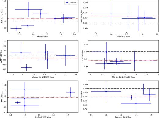
For stars with several available literature masses, the ratio of seismic to literature mass is shown, against the literature mass value. The red dotted line in each subplot is the average ratio of Table 3. Black dashed line is parity.

Table A1.

All available literature masses for each star in the ensemble. The values are primarily estimated from the observed spectroscopic parameters. The mass values from Huber et al. (2014) are estimated from the Hipparcos parallax.

EPIC/KIC	HD	Huber1	Johnson2	Mortier3,a	Mortier3,b	Bofanti4	Bofanti3,b	Jofré6	Maldonado7
203514293	145428	|$1.274^{+0.516}_{-0.413}$|
220548055	4313	|$1.94^{+0.039}_{-0.849}$|	1.72 ± 0.12	1.53 ± 0.09	1.35 ± 0.11	1.72 ± 0.03	1.49 ± 0.04	1.71 ± 0.13
215745876	181342	|$1.203^{+0.176}_{-0.246}$|	1.84 ± 0.13	1.7 ± 0.09	1.49 ± 0.19	1.40 ± 0.1	1.40 ± 0.1	1.78 ± 0.11	1.78 ± 0.07
220222356	5319	|$1.232^{+0.178}_{-0.250}$|		1.28 ± 0.1	1.24 ± 0.14	1.40 ± 0.1	1.2 ± 0.1
8566020	185351							1.82 ± 0.05
205924248	212771	|$1.173^{+0.154}_{-0.263}$|	1.15 ± 0.08	1.51 ± 0.08	1.22 ± 0.08	1.40 ± 0.1	1.45 ± 0.02	1.60 ± 0.13	1.63 ± 0.1
228737206	106270	|$1.447^{+0.119}_{-0.119}$|	1.32 ± 0.0922a	1.33 ± 0.05	1.33 ± 0.06	1.35 ± 0.02	1.37 ± 0.03
EPIC/KIC	HD	Wittenmyer8	Huber9	Jones10	Robinson11	Giguere12	Reffert13	Johnson14	Ghezzi15
203514293	145428	1.33 ± 0.2
220548055	4313
215745876	181342	1.42 ± 0.2		1.89 ± 0.11
220222356	5319				1.56 ± 0.18	1.51 ± 0.11
8566020	185351		|$1.684^{+0.166}_{-0.499}$|				1.73 ± 0.15	1.60 ± 0.08c	1.77 ± 0.04
								1.99 ± 0.23d
								1.90 ± 0.15e
								1.87 ± 0.07f
205924248	212771
228737206	106270

^aTsantaki et al. (2013) line list for the stars cooler than 5200 K, and the Sousa et al. (2008) line list for the hotter stars.

^bHekker & Meléndez (2007) line list

¹Huber et al. (2016).

²Johnson et al. (2010a).

^2aJohnson et al. (2011)

³Mortier et al. (2013).

⁴Bonfanti et al. (2015).

⁵Bonfanti et al. (2016).

⁶Jofré et al. (2015).

⁷Maldonado, Villaver & Eiroa (2013).

⁸Wittenmyer et al. (2016).

⁹Huber et al. (2014).

¹⁰Jones et al. (2016).

¹¹Robinson et al. (2007).

¹²Giguere et al. (2015).

¹³Reffert et al. (2015).

¹⁴Johnson et al. (2014).

^cInterferometric radius, combined with asteroseismology.

^dScaling relation, based on Δν = 15.4 ± 0.2μHz, |$\nu _{\textrm{max}}=229.8\pm 6.0 \mu$|Hz.

^e BaSTI Grid fitting with asteroseismology and SME spectroscopy.

^fGrid fitting with only SME spectroscopy, iterated with Y² grids to a converged log₁₀g.

¹⁵Ghezzi et al. (2015).