A two-point diagnostic for the H ii galaxy Hubble diagram

Abstract

A previous analysis of starburst-dominated H ii galaxies and H ii regions has demonstrated a statistically significant preference for the Friedmann–Robertson–Walker cosmology with zero active mass, known as the R_h = ct universe, over Λcold dark matter (ΛCDM) and its related dark-matter parametrizations. In this paper, we employ a two-point diagnostic with these data to present a complementary statistical comparison of R_h = ct with Planck ΛCDM. Our two-point diagnostic compares, in a pairwise fashion, the difference between the distance modulus measured at two redshifts with that predicted by each cosmology. Our results support the conclusion drawn by a previous comparative analysis demonstrating that R_h = ct is statistically preferred over Planck ΛCDM. But we also find that the reported errors in the H ii measurements may not be purely Gaussian, perhaps due to a partial contamination by non-Gaussian systematic effects. The use of H ii galaxies and H ii regions as standard candles may be improved even further with a better handling of the systematics in these sources.

galaxies: general, distance scale, large-scale structure of Universe, cosmology: observations, cosmology: theory

1 INTRODUCTION

Starbursts dominate the total luminosity of massive, compact galaxies known as HIIGx. The closely related giant extragalactic H ii regions (GEHRs) also undergo massive bursts of star formation, but tend to be located predominantly at the periphery of late-type galaxies. In both environments, the ionized hydrogen is characterized by physically similar conditions (Melnick et al. 1987), producing optical spectra with strong Balmer Hα and Hβ emission lines that are indistinguishable between these two groups of sources (Searle & Sargent 1972; Bergeron 1977; Terlevich & Melnick 1981; Kunth & Östlin 2000).

Since both the number of ionizing photons and the turbulent velocity of the gas in these objects increase as the starburst becomes more massive, HIIGx and GEHR have been recognized as possible standard candles, a rather exciting prospect given that the very high starburst luminosity facilitates their detection up to a redshift z ∼ 3 or higher (e.g. Melnick, Terlevich & Terlevich 2000; Siegel et al. 2005). The exact cause of the correlation between the luminosity L(Hβ) in Hβ and the ionized gas velocity dispersion σ is not yet fully understood, though an explanation may be found in the fact that the gas dynamics is almost certainly dominated by the gravitational potential of the ionizing star and its surrounding environment (Terlevich & Melnick 1981). These sources may therefore function as standard candles because the scatter in the L(Hβ) versus σ relation appears to be small enough for HIIGx and GEHRs to probe the cosmic distance scale independently of z (Melnick et al. 1987; Melnick, Terlevich & Moles 1988; Fuentes-Masip et al. 2000; Melnick, Terlevich & Terlevich 2000; Bosch, Terlevich & Terlevich 2002; Telles 2003; Siegel et al. 2005; Bordalo & Telles 2011; Plionis et al. 2011; Mania & Ratra 2012; Chávez et al. 2012, 2014; Terlevich et al. 2015).

Over the past several decades, HIIGx and GEHRs have been used to measure the local Hubble constant H₀ (Melnick, Terlevich & Moles 1988; Chávez et al. 2012), and to sample the expansion rate at intermediate redshifts (Melnick, Terlevich & Terlevich 2000; Siegel et al. 2005). More recently, Plionis et al. (2011) and Terlevich et al. (2015) demonstrated that the L(Hβ)–σ correlation is a viable high-z tracer, and used a compilation of 156 combined sources, including 24 GEHRs, 107 local HIIGx, and 25 high-z HIIGx, to constrain the parameters in Λcold dark matter (ΛCDM), producing results consistent with Type Ia SNe. Most recently, we (Wei et al. 2017) extended this very promising work even further by demonstrating that GEHRs and HIIGx may be utilized, not only to refine and confirm the parameters in the standard model but, perhaps more importantly, to compare and test the predictions of competing cosmologies, such as ΛCDM and the R_h = ct universe (Melia 2003, 2007, 2013a, 2016, 2017a; Melia & Abdelqader 2009; Melia & Shevchuk 2012).

These two models have been examined critically using diverse sets of data, including high-z quasars (e.g. Kauffmann & Haehnelt 2000; Wyithe & Loeb 2003; Melia 2013b, 2014; Melia & McClintock 2015b), cosmic chronometers (e.g. Jimenez & Loeb 2002; Simon, Verde & Jimenez 2005; Melia & Maier 2013; Melia & McClintock 2015a), gamma-ray bursts (e.g. Dai, Liang & Xu 2004; Ghirlanda et al. 2004; Wei, Wu & Melia 2013), Type Ia supernovae (e.g. Perlmutter et al. 1998; Riess et al. 1998; Schmidt et al. 1998; Melia 2012; Wei, Wu & Melia 2015b), and Type Ic superluminous supernovae (e.g. Inserra & Smart 2014; Wei, Wu & Melia 2015a). Their predictions have also been compared using the age measurements of passively evolving galaxies (e.g. Alcaniz & Lima 1999; Lima & Alcaniz 2000; Wei, Wu & Melia 2015c). A more complete summary of these comparisons, now based on over 20 different types of observations, may be found in table 1 of Melia (2017b).

The application of HIIGx and GEHRs as standard candles has provided one of the more compelling outcomes of this comparative study involving ΛCDM and R_h = ct (Wei, Wu & Melia 2016). Using the combined sample of Chávez et al. (2014) and Terlevich et al. (2015), we constructed the Hubble diagram extending to redshifts z ∼ 3, beyond the current reach of Type Ia SNe, and confirmed that the proposed correlation between L(Hβ) and σ is a viable luminosity indicator in both models. This sample is already large enough to demonstrate that R_h = ct is favoured over ΛCDM with a likelihood ≳ 99 per cent versus only ≲ 1 per cent, corresponding to a confidence level approaching 3σ.

These results, however, come with two important caveats, which partially motivate the complementary approach we are taking in this paper. Not surprisingly, the cosmological parameters are most sensitive to the high-z data, so the constraints resulting from this work are heavily weighted by the high-z sample of only 25 HIIGx. Given how sensitive the results are to the sub-sample of high-z HIIGx data, one would want to increase the significance of this analysis by increasing the number of HIIGx-related measurements. Indeed, with the K-band Multi Object Spectrograph at the Very Large Telescope, a larger sample of high-z HIIGx high-quality measurements may be available soon (Terlevich et al. 2015).

The second caveat attached to the analysis of Wei et al. (2017) is that we do not yet have a full grasp of the systematic uncertainties in the L(Hβ)–σ correlation; these, no doubt, impact the use of HIIGx as cosmological probes. They include the burst size, its age, the oxygen abundance of HIIGx, and the internal extinction correction (Chávez et al. 2016). An example of a non-ignorable systematic uncertainty arises from the fact that the L(Hβ)–σ relation correlates the ionizing flux from massive stars with random velocities in the potential well created by all the stars and the surrounding gas. Thus, any systematic variation in the initial mass function would alter the mass–luminosity ratio, and therefore also the zero-point and slope of the relation (Chávez et al. 2014).

In spite of the fact that the high-z sample of HIIGx is still relatively small, we can nonetheless further test the previous results by probing this compilation more deeply (than has been attempted before) using a two-point diagnostic, Δμ(z_i, z_j), defined in equa-tion (9) below. Quite generally, two-point diagnostics such as this differ from parametric fitting approaches in several distinct ways. They facilitate the comparative analysis of measurements in a pairwise fashion. One may use them with n measurements of a particular variable to generate n(n−1)/2 comparisons for each pair of data. The benefits are twofold: (1) one can test how well each pair of data fits the models, and (2) assess how closely the published error bars fit a normal distribution, thereby providing some indication of possible contamination by correlated systematic uncertainties. Zheng et al. (2016) recently used such an approach to conclude that the stated errors in cosmic chronometer data are strongly non-Gaussian, suggesting that the quoted measurement uncertainties are almost certainly not based exclusively on statistical randomness (see also Leaf & Melia 2017).

As we shall see, the diagnostic Δμ(z_i, z_j) is expected to be zero if the model being tested is the correct cosmology. To allow for possible non-Gaussianity in the published errors, we shall use both weighted-mean and median statistics to determine the degree to which each model's distribution of Δμ(z_i, z_j) values is consistent with this null result. So while Wei, Wu & Melia (2016) optimized the overall ΛCDM and R_h = ct parametric fits to the H ii galaxy Hubble diagram, here we will test the consistency of each fit with individual pairs of data. We will begin with a brief description of the data in Section 2, and then define and apply the diagnostic Δμ(z_i, z_j) in Section 3. The outcome of our analysis will be discussed in Section 4, followed by our conclusions in Section 5.

2 OBSERVATIONAL DATA AND METHODOLOGY

We base our analysis on the methodology described in Chávez et al. (2012, 2014) and Terlevich et al. (2015), using their total sample of 156 sources, including 107 local H ii galaxies, 24 GEHRs, and 25 high-z H ii galaxies. The correlation between the emission-line luminosity and the ionized gas velocity dispersion may be written as (Chávez et al. 2012; Chávez et al. 2014; Terlevich et al. 2015)

\begin{eqnarray} \log L(\mathrm{H}\beta )=\alpha \log \sigma (\mathrm{H}\beta )+\kappa {\, }, \end{eqnarray}

(1)

where α is the slope and the constant κ represents the logarithmic luminosity at log σ(Hβ) = 0. As noted, previous applications of this relation have produced a very small scatter in the correlation for L(Hβ), making it a viable luminosity indicator for cosmology. But one cannot completely avoid its cosmology dependence because the Hβ luminosity is calculated using the expression

\begin{eqnarray} L(\mathrm{H}\beta ) = 4 \pi D_L^2(z) F(\mathrm{H}\beta ){\, }, \end{eqnarray}

(2)

where D_L is the model-dependent luminosity distance at redshift z and F(Hβ) is the reddening corrected Hβ flux.

From equation (1), we may then obtain the distance modulus of an H ii galaxy according to

\begin{eqnarray} \mu _{\rm obs}=2.5\left[\kappa +\alpha \log \sigma (\mathrm{H}\beta ) - \log F(\mathrm{H}\beta )\right]-100.2 {\, }, \end{eqnarray}

(3)

with an associated error

\begin{eqnarray} \sigma _{\mu _{\rm obs}}=2.5\left[\left(\alpha \sigma _{\log \sigma }\right)^{2}+ \left(\sigma _{\log F}\right)^{2}\right]^{1/2} {\, }, \end{eqnarray}

(4)

in terms of σ_log σ and σ_log F, these being the 1σ uncertainties in log σ(Hβ) and log F(Hβ), respectively. This is to be compared with the theoretical distance modulus

\begin{eqnarray} \mu _{\rm th}\equiv 5 \log \left[\frac{D_{L}(z)}{\rm Mpc}\right]+25{\, }, \end{eqnarray}

(5)

as a function of the cosmology-dependent luminosity distance D_L.

In ΛCDM, the luminosity distance may be written

\begin{eqnarray} &&{ D_{L}^{\Lambda {\rm CDM}}(z) = {c\over H_{0}}{\, }{(1+z)\over \sqrt{| \Omega _{k}| }}{\, } {\rm sinn}\bigg \lbrace | \Omega _{k}| ^{1/2} }\nonumber\\ &&\quad\times\,\int _{0}^{z}{{\rm d}z\over \sqrt{\Omega _{\rm m}(1+z)^{3}+\Omega _{k}(1+z)^{2}+ \Omega _{\rm de}(1+z)^{3(1+w_{\rm de})}}}\bigg \rbrace,\nonumber\\ \end{eqnarray}

(6)

where p_de = w_deρ_de is the dark-energy equation of state; radiation is ignored in the local Universe. Also, Ω_i ≡ ρ_i/ρ_c, for matter (m), radiation (r), and dark energy (de), while Ω_k = 1 − Ω_m − Ω_de incorporates the spatial curvature of the Universe, and sinn is sinh when Ω_k > 0 and sin when Ω_k < 0. Today's critical density is |$\rho _c\equiv 3c^2 H_0^2/8\pi G$|⁠. Since we are here assuming a flat Universe, (i.e. Ω_k = 0), the right side of this equation becomes (1 + z)c/H₀ times the integral. For the R_h = ct cosmology (Melia 2003, 2007, 2013a, 2016a,b; Melia & Abdelqader 2009; Melia & Shevchuk 2012), the luminosity distance is given by the much simpler expression

\begin{eqnarray} D_L^{R_{\rm h}=ct}(z)={c\over H_0}(1+z)\ln (1+z){\, }. \end{eqnarray}

(7)

Here, we follow Wei, Wu & Melia (2015b, 2016) approach and circumvent circularity issues by optimizing the coefficients α and κ individually for each model, via maximization of the likelihood function. With this approach, H₀ and κ are not independent of each other; one may vary either H₀ or κ, but not both. For the purpose of maximizing the likelihood function, it is therefore useful to define a combined parameter

\begin{eqnarray} \delta \equiv -2.5\kappa -5\log H_0+125.2{\, }, \end{eqnarray}

(8)

where δ is the ‘H₀-free’ logarithmic luminosity and the Hubble constant H₀ is in units of km s^{− 1} Mpc^{− 1}. The constants α and δ are statistical ‘nuisance’ parameters, analogous to the adjustable coefficients characterizing the light curve in Type Ia SNe. The best-fitting parameters obtained in this fashion are shown in Table 1, for three models we will compare: Planck ΛCDM (Planck Collaboration XI 2016), ΛCDM with a re-optimized matter density Ω_m, and the R_h = ct universe.

Table 1.

Parameters optimized via maximization of the likelihood function.

Model	α	δ	Ωm	Ωde	wde
Rh = ct	|$4.78_{-0.09}^{+0.07}$|	|$32.01_{-0.30}^{+0.32}$|	–	–	–
Planck ΛCDM	|$4.86_{-0.08}^{+0.08}$|	|$32.27_{-0.31}^{+0.22}$|	0.3089	1.0 − Ωm	−1
ΛCDM	|$4.86_{-0.10}^{+0.09}$|	|$32.27_{-0.36}^{+0.34}$|	|$0.32_{-0.06}^{+0.09}$|	1.0 − Ωm	−1

A quick inspection of equations (3) and (5) shows that the two-point diagnostic

\begin{eqnarray} {\Delta }{\mu }{(z_i,z_j)}&\equiv& \frac{-{\delta }+2.5{\alpha }\log \sigma _i-2.5\log F_i}{5\log \left[\frac{D_L(z_i)}{1{\, }{\rm Mpc}}\right]}\nonumber\\ &&-\,\frac{-{\delta }+2.5{\alpha }\log \sigma _j- 2.5\log F_j}{5\log \left[\frac{D_L(z_j)}{1{\, }{\rm Mpc}}\right]} \end{eqnarray}

(9)

is expected to be zero for any pair of H ii data at redshifts z_i and z_j if the cosmology used to calculate D_L is correct. As one can see, the value of H₀ does not affect this constraint and is absorbed into the optimized coefficient δ. For the sake of normalizing the various quantities, however, we simply use the Planck value 67.74 km s⁻¹ Mpc⁻¹ throughout this analysis.

Notice in passing that α and δ are similar between the different cosmologies, varying between them by ≲ 4 per cent, i.e. well within 1σ. Thus, since H₀ is also not a factor in Δμ(z_i, z_j), equa-tion (9) represents a powerful diagnostic for comparing the viability of different models. The application of this two-point diagnostic will be described in the next section.

Finally, to improve the statistics even further, we have removed 17 points (including one GEHR source at z = 0.000 01) from our complete sample whose measurement places them more than 3σ away from the best-fitting curves. We have also chosen to remove the other GEHR source at z = 0.000 01. While this point is only 2σ from the best-fitting curve, it is the lowest redshift measurement in the catalogue, which, by the nature of two-point diagnostics, causes it to drastically alter the statistical results. These anomalous points are identical for all three models, so their removal does not bias either of them. The final reduced sample therefore contains 138 measurements that are used to determine the best fits reported in Table 1. The 18 eliminated sources are the two GEHRs at z = 0.000 01, and J162152+151855, J132347-013252, J211527-075951, J002339-094848, J094000+203122, J142342+225728, J094252+354725, J094254+340411, J001647-104742, J002425+140410, J103509+094516, J003218+150014, J105032+153806, WISP173-205, J084000+180531, and Q2343-BM133.

3 APPLICATION OF THE TWO-POINT DIAGNOSTIC

As discussed in more detail in Leaf & Melia (2017), the use of two-point diagnostics necessitates special care when analysing the statistics they produce. First, the weighted mean of all n(n−1)/2 Δμ(z_i, z_j) values may be calculated using the expression

\begin{eqnarray} \mu =\frac{{\Sigma _{i=1}^{n-1}{\Sigma }_{j=i+1}^{n}{\Delta }\mu (z_i,z_j)/ {\sigma }_{{\Delta }\mu _{i,j}}^2}}{{{\Sigma }_{i=1}^{n-1}\Sigma _{j=i+1}^{n}1/{\sigma }_{{\Delta \mu _{i,j}}}^2}}{\, }, \end{eqnarray}

(10)

in which |${\sigma }_{{\Delta \mu _{i,j}}}$| is the error for a single application of equa-tion (9), found using standard error propagation. The error in the mean, however, must be calculated by carefully considering the correlation introduced from the repeated use of individual points in different pairs. For this purpose, we rewrite the weighted mean in the equivalent form

\begin{eqnarray} \mu =\frac{\Sigma _{i=1}^{n}{\beta _i}M(z_i)}{{\Sigma }_{i=1}^{n-1} \Sigma _{j=i+1}^{n}1/{\sigma }_{{\Delta \mu _{i,j}}}^2}{\, }, \end{eqnarray}

(11)

with each β value given by the expression

\begin{eqnarray} \beta _i=\Sigma _{j=1}^{i-1}\frac{1}{\sigma _{\Delta \mu _{i,j}}^2}-\Sigma _{k=1+i}^{N}\frac{1}{\sigma _{\Delta \mu _{i,k}}^2}. \end{eqnarray}

(12)

In addition, we have defined the quantity

\begin{eqnarray} M(z_i)=\frac{-{\delta }+2.5{\alpha }\log \sigma _i-2.5\log F_i}{5\log \left[\frac{D_L(z_i)}{1{\, }{\rm Mpc}}\right]}. \end{eqnarray}

(13)

With the values of β thus calculated, the variance then follows and is given as

\begin{eqnarray} {\Delta }{\sigma ^2}_{\rm w.m.}=\frac{\Sigma _{i=1}^{n}{\beta ^2_i} \sigma _{M}^2(z_i)}{\left({\Sigma }_{i=1}^{n-1}\Sigma _{j=i+1}^{n}1/{\sigma }_{\Delta \mu _{i,j}}^2\right)^2}. \end{eqnarray}

(14)

Knowing the standard deviation of the mean, we now have a measure of the consistency of the measurements with a given model. In the case of the Δμ diagnostic, we expect the weighted mean to be statistically consistent with zero if the applied model is the correct cosmology. Note that we do not introduce the errors in the fitted parameters in this analysis. This is due to the error affecting both halves of the two-point diagnostics in a very similar manner. That is, if the value of α is slightly too low, it would have the effect of reducing both ‘single-points’, the net effect of which ends up being statistically insignificant.

When non-Gaussian errors are suspected, however, such situations motivate the use of ‘median statistics’, pioneered by Gott et al. (2001), in which error propagation is neither required nor assumed. This approach takes advantage of the fact that for any measurement based on some distribution function, there is a 50 per cent chance of it being above the true median of the underlying distribution, without any need to know its form. Thus, for N ranked measurements, the true median has a probability

\begin{eqnarray} P_i=\frac{2^{-N}N!}{i!(N-i)!} \end{eqnarray}

(15)

(i.e. the binomial distribution) of being found between measurements i and i + 1. One can use this to construct confidence regions about the median of the data, analogous to a standard deviation in Gaussian statistics, and assign to them a formal probability of finding the true median of the underlying distribution. However, it would be incorrect to apply this to, say all n(n−1)/2 diagnostics at once, for the same reasons noted in Leaf & Melia (2017). The fact that each measurement contributes to N − 1 diagnostics means that the data are correlated; as a result, a single measurement can move the median farther than in the case where the two-point values are truly randomly distributed.

We propose a remedy that takes advantage of the binomial properties of the median, but instead of considering all the diagnostics simultaneously, we construct a random sub-sample, in which each realization of the diagnostic is used exactly once, except for the one that was omitted. Therefore, none of the diagnostic values is used more than once, completely avoiding any possible correlation. Following this, we record the median of the diagnostics of this uncorrelated sample, as well as the standard deviation of the realization. Next, we generate a large number (here, one million) of these realizations, and report the overall median of all the individual medians in Table 2.

Table 2.

Statistical analysis of the two-point diagnostic Δμ(z_i, z_j).

Model	Weighted mean	1σ error	|Mean| / σ	|Nσ| < 1	Median	Std. Dev. of the median	|Median| / Std. Dev.
Rh = ct	−0.00242	0.00218	1.11	51.3 per cent	−0.00425	0.00336	1.26
Planck ΛCDM	−0.00340	0.00221	1.54	52.3 per cent	−0.00483	0.00363	1.33
ΛCDM	−0.00330	0.00220	1.50	52.2 per cent	−0.00476	0.00342	1.39

In Table 2, we also report the standard deviation of the median. This value is different from the overall standard deviation of the set of all one million medians. It is fundamentally related to the error in the mean of any set of data, in that it is some distinct factor smaller than the standard deviation of the data, dependent on the size of the data set. However, the exact relationship that exists between the standard deviation of the medians and the number of sources used to determine the median of all the realizations is not empirically known.

In order to address this deficiency, we have used the following approach, based on Monte Carlo simulations with mock data to find this relationship to reasonable accuracy. We construct a mock data set by drawing at random from some probability distribution function, with the same number (i.e. 138) of points as in the real data set. Then, we construct a random set of two-point diagnostics following the same method used with the real data. We record the median and standard deviation of the realization, repeating this process a sufficiently large number of times (say, 20 000). Then, we repeat the process with a new random set of mock data drawn from the same distribution, and repeat this 5000 times. Next, we determine the standard deviation of the set of 5000 medians, as well as the mean of the 5000 standard deviations. Finally, we compare the actual standard deviation of the median of all realizations with the mean of the standard deviations of each realization. We run this simulation with three different probability density functions: a normal distribution, a skew normal distribution with shape parameter α = 4, and a flat distribution over an interval. In all three cases, the relationship between the standard deviation of the median and the mean standard deviation of each realization is found to be statistically consistent, and apparently dependent only on the number of sources chosen.

For a sample of 138, the multiplicative factor is 1.822, always yielding a standard deviation of the medians smaller than the mean of the standard deviations by this factor. The values reported in Table 2 for the standard deviation of the median are therefore determined by taking the standard deviations of the million medians and dividing them by the corresponding factor. While this does technically include an implicit assumption that all data are sampled from a single underlying statistical distribution, we argue that by focusing on the median of these (instead of the mean), and the fact that there must certainly exist a single true cosmological model, this assumption is reasonable.

The two-point diagnostic we have introduced in equation (9) is expected to be zero for the correct cosmology. The degree by which a given model's median is consistent with zero is therefore a measure of its consistency with the observations. We discuss the results of this analysis in the next section.

4 DISCUSSION

In Table 2 and Figs 1 –6, we report the results of both our weighted-mean and median statistical analyses, described in Sections 2 and 3 above. One of the principal benefits of two-point diagnostics constructed with regard to redshift ordering lies not only in determining how well a set of data fits a model, as revealed, e.g. with the use of information criteria but, also in providing insight into whether or not the low-z sources are consistent with the same model as that preferred by the higher-z sources.

Figure 1.

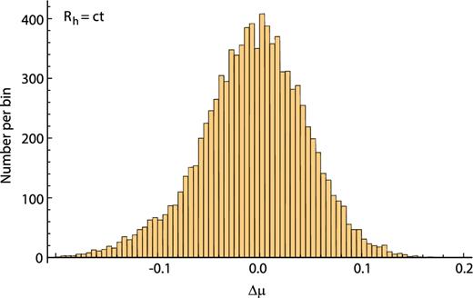
Unweighted histogram of all 9453 Δμ diagnostic values for the R_h = ct universe (see equation 9). The y-axis gives the number of diagnostic values per bin.

Figure 2.

Same as Fig. 1, except now for Planck ΛCDM.

Figure 3.

Same as Fig. 1, except now for ΛCDM with a re-optimized value of Ω_m (see Table 1).

Figure 4.

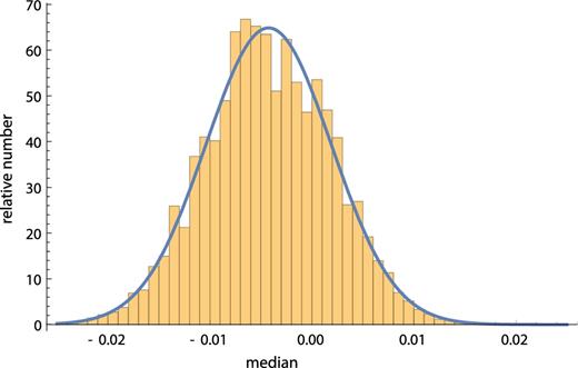
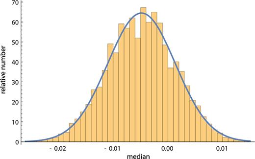
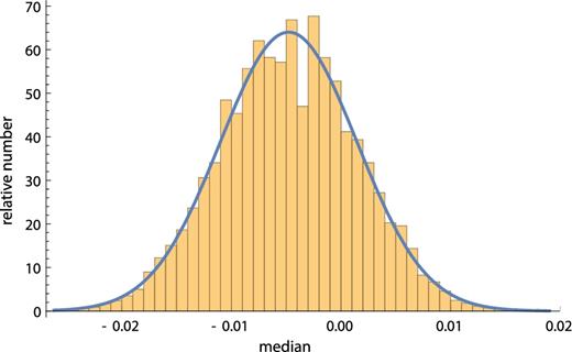
Histogram of the medians found in one million random realizations of the two-point diagnostic for the R_h = ct universe. The y-axis denotes the number of times (×1000) that the median of a realization falls within the range given on the x-axis.

Figure 5.

Same as Fig. 4, except for Planck ΛCDM.

Figure 6.

Same as Fig. 4, except for ΛCDM with a re-optimized Ω_m, as indicated in Table 1.

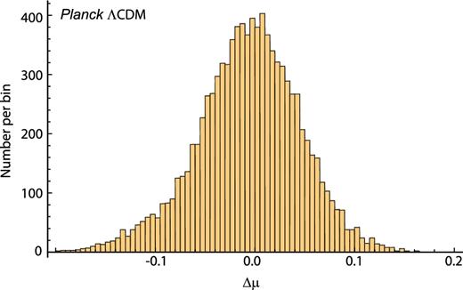
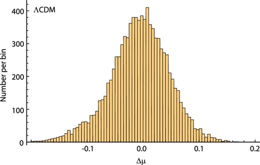
Our complete sample of 138 sources constitutes the original 156 minus the 18 outliers, as detailed in Section 2. As one can see from Table 1, the optimized value of α is about 4.8 in every case, statistically consistent with the results of previous analyses by Chávez et al. (2012, 2014), Terlevich et al. (2015), and Wei, Wu & Melia (2016). For these 138 measurements, we constructed for each model the 9453 unique two-point diagnostics and calculated the weighted mean and corresponding 1σ error based on the reported uncertainties (see Figs 1–3 for the complete unweighted histograms). For the R_h = ct universe (Fig. 4), the weighted mean is found to be consistent with zero at about 1σ. There is mild tension for Planck ΛCDM (Fig. 5) and the best-fitting ΛCDM cosmology (Fig. 6), however, in that the weighted mean is inconsistent with zero at about 1.5σ (compare the entries in columns 2, 3, and 4 of Table 2). Perhaps more importantly, fewer than the expected 68.3 per cent of the diagnostics lie within 1σ of the weighted mean (column 5) for all three models, implying that the reported errors are probably not purely Gaussian and that there may be an additional source of error not accounted for in this analysis.

It is therefore helpful to circumvent this possible non-Gaussianity by also analysing the two-point diagnostics using median statistics, as described above. With this approach, the three models show a similar inconsistency with a zero median (columns 5 and 6 of Table 2), with a negative value in every case, roughly 1.3σ different from zero. The fact that both the weighted mean and the median are negative for all the models suggests that the luminosity distance at low-z is generally greater than that predicted by these cosmologies, or that it is smaller than expected at high-z. The implication is that either (i) none of the models are completely correct, or (ii) there may be some systematic problems with the data at high-z or (more likely) at low-z. Thus, while a discrepancy smaller than 2σ may not be definitive, it nonetheless motivates further analysis involving a possible contamination by non-Gaussian systematic errors.

Along these lines, we point out that some authors have speculated on the possibility that a local ‘Hubble bubble’ (Shi 1997; Keenan, Barger & Cowie 2013; Romano 2017) might be influencing the local dynamics within a distance ∼300 Mpc (i.e. z ≲ 0.07). If true, such a fluctuation might lead to anomalous velocities within this region, causing the nearby expansion to deviate somewhat from a pure Hubble flow. This effect could be the reason we are seeing a slight negative bias for the weighted mean and median of the two-point diagnostic for every model, since nearby velocities would be slightly larger than Hubble, implying larger than expected luminosity distances at redshifts smaller than ∼0.07. In addition, the existence of local peculiar velocities would imply that the errors associated with low-z measurements should be bigger than quoted, increasing the number of two-point diagnostics that fall within 1σ of the expected dispersion, possibly ‘filling’ the distributions in Figs 1–3 sufficiently to produce entries in column 5 of Table 2 closer to the value ( ∼ 68.3 per cent) expected of a true Gaussian distribution.

5 CONCLUSIONS

The totality of the results shown in Tables 1 and 2, and illustrated in Figs 1–6, supports the use of HIIGx and GEHR sources as standard candles for cosmological testing, though the analysis based on two-point diagnostics has probed the measurement errors in greater detail than was possible solely via parametric fits to the data, the subject of our previous paper on this subject (Wei, Wu & Melia 2016).

In this paper, we have proposed a new two-point diagnostic for analysing HIIGx and GEHR data with the inclusion of median statistics, which circumvents the need for assuming Gaussian errors in the measurements. This approach may be used alongside, and compared, with the better understood weighted mean method. We have shown that these two types of analyses give generally consistent results, insofar as the H ii data are concerned. Broadly speaking, one of the principal conclusions of this analysis is that employing the entire compilation of HIIGx and GEHR sources (with the exception of several outliers) produces slight tension between the cosmological parameters favoured by the data at low and high redshifts. We believe this is circumstantial evidence in support of the proposal by Shi (1997), Keenan, Barger & Cowie (2013) and Romano (2017) of a dynamical influence due to a local Hubble bubble extending out to z ∼ 0.07, which produces local peculiar velocities comparable to those in the Hubble flow at low redshifts.

Nonetheless, probing the HIIGx and GEHR data with two-point diagnostics has not changed the essential conclusions drawn by Wei, Wu & Melia (2016), whose cosmological tests based on these sources favoured the R_h = ct model over ΛCDM. Our comparison using the H ii sample has shown that R_h = ct is favoured over both Planck ΛCDM and ΛCDM with a variable Ω_m, at least when viewed in terms of weighted mean statistics. The caveat, however, is that an approach based on median statistics produces less differentiation between the three models.

In addition, we have found in all cases that our two-point diagnostic with the weighted mean approach yields fewer values within individual 1σ error regions than the 68.3 per cent required of a true Gaussian distribution. This may be an indication that the reported errors are not purely statistical, which may happen, e.g. when the uncertainties are contaminated by systematic effects, including at least a partially non-Gaussian component, or when there is an additional source of uncertainty, other than what we considered in this analysis.

Acknowledgements

We are very grateful to the anonymous referee for providing valuable insights and suggesting improvements to the manuscript. FM is supported by Chinese Academy of Sciences Visiting Professorships for Senior International Scientists under grant 2012T1J0011, and the Chinese State Administration of Foreign Experts Affairs under grant GDJ20120491013.