NGTS-4b: A sub-Neptune transiting in the desert

Abstract

We report the discovery of NGTS-4b, a sub-Neptune-sized planet transiting a 13th magnitude K-dwarf in a 1.34 d orbit. NGTS-4b has a mass M = 20.6 ± 3.0 M_⊕ and radius R = 3.18 ± 0.26 R_⊕, which places it well within the so-called ‘Neptunian Desert’. The mean density of the planet (3.45 ± 0.95 g cm⁻³) is consistent with a composition of 100  per cent H₂O or a rocky core with a volatile envelope. NGTS-4b is likely to suffer significant mass loss due to relatively strong EUV/X-ray irradiation. Its survival in the Neptunian desert may be due to an unusually high-core mass, or it may have avoided the most intense X-ray irradiation by migrating after the initial activity of its host star had subsided. With a transit depth of 0.13 ± 0.02 per cent, NGTS-4b represents the shallowest transiting system ever discovered from the ground, and is the smallest planet discovered in a wide-field ground-based photometric survey.

techniques: photometric, planets and satellites: detection, stars: individual: NGTS-4– planetary systems

1 INTRODUCTION

Exoplanet population statistics from the Kepler mission reveals a scarcity of short-period Neptune-sized planets (Szabó & Kiss 2011; Mazeh, Holczer & Faigler 2016; Fulton & Petigura 2018). This so-called ‘Neptunian Desert’ is broadly defined as the lack of exoplanets with masses around 0.1 M_J and periods less than 2–4 d (Szabó & Kiss 2011). As Neptune-sized planets should be easier to find in short-period orbits, and many Neptunes have been discovered with longer orbits from surveys such as CoRoT and Kepler, this does not appear to be an observational bias. Ground-based surveys, which have uncovered the bulk of known hot Jupiters, have not uncovered these short-period Neptunes. However this may be due to the fact that such exoplanets produce transits too shallow for most ground-based surveys to detect.

The physical mechanisms that result in the observed Neptunian Desert are currently unknown, but have been suggested to be due to a different formation mechanism for short-period superEarth, and Jovian exoplanets, similar to the reasons for the brown dwarf desert (e.g. Grether & Lineweaver 2006). Alternatively, the dearth may be due to a mechanism stopping planetary migration. This may be a sudden loss of density within the accretion disc or mass removed from the exoplanet via Roche lobe overflow (Kurokawa & Nakamoto 2014), or stellar X-ray/EUV insolation (Lopez & Fortney 2014) and evaporation of the atmosphere (Lecavelier Des Etangs 2007).

Owen & Lai (2018) investigated causes of the high-mass/large radius and low-mass/small radius boundaries of the desert. They showed that while X-ray/EUV photoevaporation of sub-Neptunes can explain the low-mass/small radius boundary, the high-mass/large radius boundary better corresponds to the tidal disruption barrier for gas giants undergoing high-eccentricity migration. Their findings were consistent with the observed triangular shape of the desert, since photoevaporation is more prolific at shorter orbital periods, likewise more massive gas giants can tidally circularize closer to their stellar hosts.

Due to their shallow transits, Neptune-sized planets (≈4 R_⊕) have largely eluded wide-field ground-based transit surveys such as WASP (Pollacco et al. 2006), HATNet (Bakos et al. 2004), HATSouth (Bakos et al. 2013), and KELT (Pepper et al. 2007, 2012). The notable exception is HAT-P-11b (Bakos et al. 2010), which has a radius of just 4.71 ± 0.07 R_⊕. One other system worthy of note is the multiplanet system TRAPPIST-1 (Gillon et al. 2016), of which three of the Earth-sized planets were discovered from ground; however, they orbit a late M-dwarf and their transit depths are in the range 0.6–0.8 per cent (5–6 times larger than the depth of NGTS-4b), and surveys such as TRAPPIST and MEarth (Nutzman & Charbonneau 2008; Irwin et al. 2009) have specifically targeted M-dwarfs in order to maximize the detectability of small planets.

We present the discovery of a new sub-Neptune-sized (R = 3.18 ± 0.26 R_⊕) planet transiting a K-dwarf (m_v = 13.1 mag) in a P = 1.337 34 d orbit from the Next Generation Transit Survey (NGTS) survey. In Section 2 we describe the NGTS discovery data. In Section 3 we describe our campaign of photometric follow-up on 1 m-class telescopes. In Section 4 we detail our spectroscopic follow-up including the mass determination via radial velocity monitoring. In Section 5 we discuss our analysis of the stellar parameters and describe the global modelling process. In Section 6 we discuss the discovery in context with other planets in this mass, radius, or period regime. Finally, we finish with our conclusions in Section 7.

2 DISCOVERY PHOTOMETRY FROM NGTS

NGTS-4 was observed using a single NGTS camera over a 272 night baseline between 2016 August 06 and 2017 May 05. The survey has operated at ESO’s Paranal observatory since early 2016 and consists of an array of 12 roboticized 20 cm telescopes. The facility is optimized for detecting small planets around K and early M stars (Chazelas et al. 2012; Wheatley et al. 2013; McCormac et al. 2017; Wheatley et al. 2018).

A total of 190  696 images were obtained, each with an exposure time of 10 s. The data were taken using the custom NGTS filter (550–927 nm) and the telescope was autoguided using an improved version of the DONUTS autoguiding algorithm (McCormac et al. 2013). The RMS of the field tracking errors was 0.051 pixels (0.26 arcsec) over the 272 night baseline. The data were reduced and aperture photometry was extracted using the casutools¹ photometry package. A total of 185 840 valid data points were extracted from the raw images. The data were then de-trended for nightly trends, such as atmospheric extinction, using our implementation of the SysRem algorithm (Tamuz, Mazeh & Zucker 2005; Collier Cameron et al. 2006). We refer the reader to Wheatley et al. (2018) for more details on the NGTS facility and the data acquisition and reduction processes.

The complete data set was searched for transit-like signals using orion, an optimized implementation of the box-fitting least-squares algorithm (Kovács, Zucker & Mazeh 2002; Collier Cameron et al. 2006), and a ∼0.2  per cent signal was detected at a period of 1.337 34 d. The NGTS photometry, phase-folded to this period, is shown in Fig. 1. A total of 28 transits are covered fully or partially by the NGTS data set.

Figure 1.

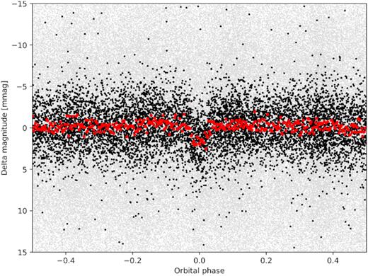
The NGTS discovery light curve of NGTS-4b. The data are shown phase-folded on the orbital period 1.337 34 d. The grey points show the unbinned 10 s cadence data, the black dots are these data binned in linear time to a cadence of 5 min then phase-folded, and the red points are the unbinned data phase-folded then binned in phase to an equivalent cadence of 5 min.

We find no evidence for a secondary eclipse or out-of-transit variation, both of which would indicate an eclipsing binary system. We used the centroid vetting procedure detailed in Günther et al. (2017) to check for contamination from background objects, and verify that the transit seen was not a false-positive. This test is able to detect shifts in the photometric centre of flux during transit events at the sub-milli-pixel level. It can identify blended eclipsing binaries at separations below 1 arcsec, well below the size of individual NGTS pixels (5 arcsec). We find no signs of a centroiding variation during the transit events of NGTS-4.

Based on the NGTS detection and the above vetting tests, NGTS-4 was followed up with further photometry and spectroscopy to confirm the planetary nature of the system and measure the planetary parameters. A sample of the full discovery photometry and follow-up data is given in Table 1, the full data are available in machine-readable format from the online journal.

Table 1.

Summary of NGTS photometry of NGTS-4. A portion is shown here for guidance. The full table along with photometry from Eulercam, LCO 1m, SPECULOOS, and SHOCa is available in a machine-readable format from the online journal.

BJDTDB	Relative	Flux	Filter	Instrument
(−2400000.0)	flux	error
57 650.788 430 95	1.013 51	0.011 43	NGTS	NGTS
57 650.788 580 95	1.000 41	0.011 40	NGTS	NGTS
57 650.788 730 95	0.998 46	0.011 42	NGTS	NGTS
57 650.788 880 95	1.013 30	0.011 46	NGTS	NGTS
57 650.789 030 95	0.990 49	0.011 41	NGTS	NGTS
57 650.789 170 95	1.003 62	0.011 43	NGTS	NGTS
57 650.789 320 95	0.993 64	0.011 42	NGTS	NGTS
57 650.789 470 95	0.999 04	0.011 41	NGTS	NGTS
57 650.789 620 95	1.009 97	0.011 44	NGTS	NGTS
57 650.789 770 95	0.988 00	0.011 38	NGTS	NGTS
57 650.789 920 95	1.003 27	0.011 44	NGTS	NGTS
57 650.790 070 95	1.004 83	0.011 43	NGTS	NGTS
...	...	...	...	...

3 PHOTOMETRIC FOLLOW-UP

Confirming such a shallow transit signal from the ground is challenging, even given some of the best 1 m-class telescopes available for precision time-series photometry. We therefore undertook a campaign of photometric follow-up using four different facilities as set out in this section. A summary of the photometric follow-up observations is given in Table 2, and the full data are available in machine-readable format in the online journal. The de-trended data are plotted in Fig. 4 (see Section 5.2 for a description of the de-trending that has been applied to the data in these plots).

Table 2.

A summary of the follow-up photometry of NGTS-4.

Night	Site	Instrument	Nimages	Exptime	Binning	Filter	Comment
				(s)
2017 Nov 27	SAAO	SHOC	360	30	4 × 4	V	Full transit
2018 Apr 15	CTIO	LCO 1m	31	180	1 × 1	i	Mid + egress
2018 Apr 15	Paranal	Speculoos/Callisto	471	12	1 × 1	I + z	Full transit
2018 Apr 15	Paranal	Speculoos/Europa	473	12	1 × 1	I + z	Full transit
2018 Apr 15	La Silla	Eulercam	193	40	1 × 1	NGTS	Full transit
2018 Apr 16	SSO	LCO 1m	19	180	1 × 1	i	Egress
2018 Apr 19	CTIO	LCO 1m	11	180	1 × 1	i	Ingress
2018 Apr 19	La Silla	Eulercam	140	55	1 × 1	NGTS	Full transit
2018 Apr 20	SSO	LCO 1m	16	180	1 × 1	i	Egress
2018 Apr 22	SAAO	SHOC	2160	2	4 × 4	I	Egress
2018 Apr 27	CTIO	LCO 1m	19	180	1 × 1	i	Egress
2018 May 06	SSO	LCO 1m	15	180	1 × 1	i	Egress

3.1 SHOC photometry

Our first follow-up photometry of NGTS-4 was carried out at the South African Astronomical Observatory (SAAO) on 2017 November 27, with the 1.0 m telescope and one of the three frame-transfer CCD Sutherland High-speed Optical Cameras (SHOC Coppejans et al. 2013), specifically SHOC’n’awe. The SHOC cameras on the 1 m telescope have a pixel scale of 0.167 arcsec pixel⁻¹, which is unnecessarily fine for our observations, hence we binned the camera 4 × 4 pixels in the X and Y directions. All observations were obtained in focus, using a V filter and an exposure time of 30 s. The field of view of the SHOC instruments on the 1 m is 2.85 × 2.85 arcmin, which allowed for one comparison star of similar brightness to the target to be simultaneously observed.

The data were bias and flat-field corrected via the standard procedure using the ccdproc package (Craig et al. 2015) in python. Aperture photometry was extracted for NGTS-4 and the comparison star using the sep package (Bertin & Arnouts 1996; Barbary 2016) and the sky background was measured and subtracted using the sep background map. We also performed aperture photometry using the Starlink package autophotom. We used a 4 pixel radius aperture that maximized the signal or noise, and the background was measured in an annulus surrounding this aperture. The comparison star was then used to perform differential photometry on the target. Both photometry methods successfully detected a complete transit of NGTS-4b despite the observations being partially effected by thin cirrus during the transit.

NGTS-4 was observed again at SAAO with the 1 m telescope and the SHOC’n’awe instrument at the end of astronomical twilight on 2018 April 22. On this occasion sky conditions were excellent, with sub-arcsec seeing throughout and a minimum of ≈0.6 arcsec recorded. On this occasion the observations were made using an I filter. Initially, an exposure time of 5 s was used, but after the first 30 min this was reduced to 2 s as the target’s flux was uncomfortably close to the non-linear regime of the CCD. These data were also reduced and analysed as described above, and the transit egress was clearly detected (Fig. 4).

3.2 LCO 1 m

We monitored transit events of NGTS-4b using the Las Cumbres Observatory (LCO) 1 m global telescope network (Brown et al. 2013). All observations were taken using the Sinistro cameras, which given a 26.5 × 26.5 arcmin field of view with a plate-scale of 0.389 arcsec pixel⁻¹. Exposure times were set to 180 s, with a defocus of 2 mm in order to ensure we did not saturate NGTS-4 and light was spread over a larger number of detector pixels. We used the i-band filter and the standard 1 × 1 binning readout mode. In total six events were monitored with the LCO 1 m telescopes from the sites in Chile and Australia. A full list of these events along with details of each observation are set out in Table 2.

Raw images were reduced to calibrated frames using the standard LCO ‘Banzai’ pipeline. Aperture photometry was extracted for NGTS-4 and the seven comparison stars using the sep package (Bertin & Arnouts 1996; Barbary 2016), and the sky background was measured and subtracted using the sep background map. The resulting light curve shows the signature of a full transit (Fig. 4).

3.3 Speculoos

We monitored a transit event using the SPECULOOS-South facility (Burdanov et al. 2017; Delrez et al. 2018) at Paranal Observatory in Chile on the night of 2018 April 15, taking advantage of the telescope commissioning period. SPECULOOS-South consists of four robotic 1 m Ritchey–Chretien telescopes, and we were able to utilize two of these (Europa and Callisto) to observe the transit event. Given the shallowness of the targeted transit, we opted to maximize the flux from the early K host star and chose an I + z filter for both telescopes. SPECULOOS-South is equipped with a deep-depletion 2 × 2 k CCD camera with a field of view of 12 × 12 arcmin (0.35 arcsec pixel⁻¹).

The images were calibrated using standard procedures (bias, dark, and flat-field correction) and photometry was extracted using the iraf or daophot aperture photometry software (Stetson 1987), as described by Gillon et al. (2013). For each observation, a careful selection of both the photometric aperture size and stable comparison stars was performed manually to obtain the most accurate differential light curve of NGTS-4. The signature of a full transit is evident in the light curves from both telescopes (Fig. 4).

3.4 Eulercam

Two transits of NGTS-4 were observed with Eulercam on the 1.2 m Euler Telescope at La Silla Observatory (Lendl et al. 2012). The observations took place on the nights beginning 2018 April 15 and 2018 April 19. Both transits were observed using the same broad NGTS filter that was used to obtain the discovery photometry. For the first observation a total of 193 images were obtained using a 40 s exposure and 0.1 mm defocus. For the second observation a total of 140 images were obtained using a 55 s exposure time and 0.1 mm defocus.

The data were reduced using the standard procedure of bias subtraction and flat-field correction. Aperture photometry was performed with the pyraf implementation of the phot routine. pyraf was also used to extract information useful for de-trending; X- and Y-position, full width at half-maximum (FWHM), airmass, and sky background of the target star. The comparison stars and the photometric aperture radius were chosen in order to minimize the RMS in the scatter out of transit. Additional checks were made with different comparison star ensembles, aperture radii, and with stars in the FOV expected to show no variation. This was to ensure the transit signal was not an artefact of these choices. The resulting light curves are plotted in Fig. 4, showing a detection of a full transit signature in the data from 2018 April 19, though the detection in the data from 2018 April 15 is marginal at best.

4 SPECTROSCOPY

We obtained multi-epoch spectroscopy for NGTS-4 with the HARPS spectrograph (Mayor et al. 2003) on the ESO 3.6 m telescope at La Silla Observatory, Chile, between 2017 December 01 and 2018 April 10 under programme ID 0101.C-0623(A).

We used the standard HARPS data reduction software to measure the radial velocity of NGTS-4 at each epoch. This was done via cross-correlation with the K0 binary mask. The exposure times for each spectrum were 2700 s. The radial velocities are listed, along with their associated error, FWHM, contrast, bisector span, and exposure time in Table 3.

Table 3.

HARPS radial velocities for NGTS-4. These data are available in machine-readable format from the online journal.

BJDTDB	RV	RV err	FWHM	Contrast	BIS	Exptime
(−2400 000.0)	(km s−1)	(km s−1)	(km s−1)		(km s−1)	(s)
58 088.796 126	111.203 32	0.004 28	6.052 96	42.601	−0.029 45	2700
58 090.790 319	111.202 80	0.006 29	6.024 78	40.836	−0.005 21	2700
58 091.804 515	111.222 90	0.004 92	6.056 77	41.368	−0.042 56	2700
58 113.827 181	111.187 89	0.003 90	6.034 59	42.909	−0.016 15	2700
58 125.694 569	111.191 85	0.003 45	6.060 11	42.884	−0.015 53	2700
58 127.682 623	111.202 92	0.008 28	6.028 70	42.492	−0.037 70	2700
58 160.714 908	111.204 32	0.005 74	6.011 84	42.535	−0.032 20	2700
58 162.719 953	111.217 67	0.006 39	6.037 78	42.665	−0.035 07	2700
58 189.543 826	111.212 05	0.004 56	6.039 51	43.090	−0.023 21	2700
58 190.545 562	111.212 05	0.005 12	6.056 74	42.993	−0.003 93	2700
58 199.563 729	111.186 39	0.004 63	6.055 06	42.778	−0.052 51	2700
58 215.559 376	111.196 00	0.007 10	6.045 39	43.125	−0.051 81	2700
58 216.556 670	111.196 22	0.005 19	6.035 21	43.087	−0.033 27	2700
58 218.564 257	111.195 22	0.008 70	6.082 29	43.049	0.003 62	2700

The 14 radial velocity measurements show a variation in-phase with the period detected by orion. With a semi-amplitude of 13.7 ± 1.9 m s⁻¹ they indicate a Neptune-mass transiting planet (see Fig. 2). To ensure that the radial velocity signal originates from a planet orbiting NGTS-4, we analysed the HARPS cross-correlation functions (CCF) using the line bisector technique of Queloz et al. (2001). We find no evidence for a correlation between the radial velocity and the bisector spans (see Fig. 3).

Figure 2.

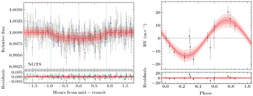
Left: De-trended NGTS discovery photometry with the gp-ebop model’s transit component in red. The data are binned to 10 min cadence, with individual transits colour-coded. Right: HARPS radial velocity data with the best-fitting circular orbit model. In both cases, the red lines and pink shaded regions show the median and the 1 and 2σ confidence intervals of gp-ebop’s posterior model.

Figure 3.

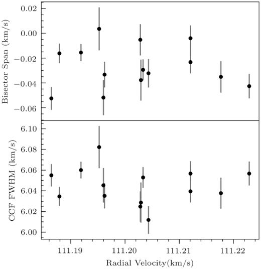
Top: HARPS CCF bisector slopes for the spectra in Table 3, plotted against radial velocity. We find no trend in the bisectors with radial velocity, which can be indicative of a blended system. Bottom: CCF FWHM for the same HARPS spectra. The FWHM of the HARPS CCFs are essentially constant.

In order to characterize the stellar properties of NGTS-4 we wavelength shift and combine all 14 HARPS spectra to create a high signal-to-noise spectrum for analysis in Section 5.1.

5 ANALYSIS

5.1 Stellar properties

5.1.1 Spectroscopic stellar parameters

The HARPS spectra were analysed using species (Soto & Jenkins 2018). This is a python tool to derive stellar parameters in an automated way, from high-resolution echelle spectra. species measures the equivalent widths (EWs) for a list of FeI and FeII lines using ares (Sousa et al. 2015), and they are input into moog (Sneden 1973), along with atlas9 model atmospheres (Castelli & Kurucz 2004), to solve the radiative transfer equation. The correct set of atmospheric parameters (T_eff, log g, [Fe/H]) are reached when no correlations exist between the obtained abundances for each line, the line excitation potential, and the reduced EW (EW/λ), and the abundance of neutral and ionized iron agree. Mass and radius are found by interpolating through a grid of MIST isochrones (Dotter 2016), using a Bayesian approach. The atmospheric parameters, along with the extinction-corrected magnitudes and the Gaia parallax listed in Table 4, were used as priors. The extinction for each band was computed using the maps from Bovy et al. (2016). Finally, the rotational and macroturbulent velocity were derived using the relation from dos Santos et al. (2016), and by line fitting to a set of five absorption lines. species gives a stellar radius of 0.84 ± 0.01 R_⊙ and a metallicity of −0.28 ± 0.10 dex. The stellar parameters measured by species are listed in Table 4.

Table 4.

Stellar Properties for NGTS-4.

Property	Value	Source
Astrometric properties
RA	|$05^{\rm{h}} 58^{\rm{m}} 23{^{\rm s}_{.}}76$|	2MASS
Dec.	−30°48′42|${^{\prime\prime}_{.}}$|49	2MASS
2MASS I.D.	05 582 375–304 8424	2MASS
Gaia source I.D.	2891 248 292 906 892 032	Gaia DR2
μRA (mas yr−1)	−16.881 ± 0.034	Gaia DR2
μDec. (mas yr−1)	−7.371 ± 0.036	Gaia DR2
γgaia (km s−1)	110.5 ± 5.5	Gaia DR2
Parallax (mas)	3.536 ± 0.023	Gaia DR2
Distance (parsec)	282.6 ± 1.8	Gaia DR2
Photometric properties
V (mag)	13.14 ± 0.03	APASS
B (mag)	13.95 ± 0.05	APASS
g (mag)	13.48 ± 0.02	APASS
r (mag)	12.91 ± 0.07	APASS
i (mag)	12.64 ± 0.09	APASS
G (mag)	12.91	Gaia DR2
GRP (mag)	12.31	Gaia DR2
GBP (mag)	13.36	Gaia DR2
NGTS (mag)	12.59 ± 0.01	This work
J (mag)	11.58 ± 0.02	2MASS
H (mag)	11.14 ± 0.02	2MASS
K (mag)	11.07 ± 0.02	2MASS
W1 (mag)	11.03 ± 0.02	WISE
W2 (mag)	11.09 ± 0.02	WISE
W3 (mag)	10.98 ± 0.11	WISE
Derived Properties
Teff (K)	5143 ± 100	species
[M/H]	−0.28 ± 0.10	species
vsin i (km s−1)	2.75 ± 0.58	species
γRV (km s−1)	111.2 ± 0.2	Global modelling
log g	4.5 ± 0.1	species
M*(M⊙)	0.75 ± 0.02	species
R*(R⊙)	0.84 ± 0.01	species
ρ* (g cm−3)	1.79 ± 0.14	species
vmac	1.40 ± 0.58	species
Distance (pc)	282.6 ± 1.8	Gaia DR2

2MASS (Skrutskie et al. 2006); WISE (Wright et al. 2010);

APASS (Henden & Munari 2014);

Gaia DR2 (Gaia Collaboration et al. 2018a)

and Mann et al. (2015)

5.1.2 Kinematics and environment

Using the Gaia parallax and the tables of Bailer-Jones et al. (2018), we estimate the distance to NGTS-4 to be 282.6 ± 1.8 parsec.

NGTS-4 has a relatively high proper motion, consistent with what we expect for the estimated distance and spectral-type, of −16.881 ± 0.034 mas yr⁻¹ and −7.371 ± 0.036 mas yr⁻¹ in RA and Dec., respectively. It has a very high systemic radial velocity as determined from our HARPS observations (111.2 ± 0.2 km s⁻¹) and confirmed from Gaia DR2 (110.5 ± 5.5 km s⁻¹).

When combined with the Gaia DR2 parallax (Gaia Collaboration 2018a), we derived the following Galactic velocity components (U_LSR, V_LSR, W_LSR) with respect to the local standard of rest (LSR) to be (66.99 ± 0.10, −72.46 ± 0.15, −38.22 ± 0.08) km s⁻¹, assuming the LSR is UVW = (11.1, 12.24, 7.25) km s⁻¹ from Schönrich, Binney & Dehnen (2010). This suggests that NGTS-4 is a member of the thick disc population (V_tot = 105.8 km s⁻¹, see e.g. Gaia Collaboration et al. 2018b) similar to NGTS-1 (Bayliss et al. 2018).

There are no other sources within 15 arcsec of NGTS-4 in the Gaia DR2 catalogue. This means we can rule out any blended object down to a Gaia magnitude of approximately G = 20.7 beyond 2 arcsec and within the NGTS photometric aperture. However, the Gaia DR2 completeness for close companions falls off within 2 arcsec and is zero within 0.5 arcsec (Arenou et al. 2018).

5.2 Global modelling

To obtain fundamental parameters for NGTS-4b, we modelled the light and radial velocity curves of NGTS-4 using gp-ebop (Gillen et al. 2017). These comprise the NGTS discovery light curve, 12 follow-up light curves from six 1m-class telescopes, and 14 HARPS RVs (as set out in Sections 2, 3, and 4). gp-ebop comprises a central transiting planet and eclipsing binary model, which is coupled with a Gaussian process (GP) model, and wrapped within a Markov Chain Monte Carlo (MCMC). Limb darkening (LD) is incorporated using the analytic method of Mandel & Agol (2002), for the quadratic law with the profiles and uncertainties constrained by the predictions of LDtk (Parviainen & Aigrain 2015).

Most stars are intrinsically variable, which can affect the apparent shape and depth of planet transits. The more active the star or the higher the level of instrumental systematics, or the shallower the transit signal, the greater the effect on the transit modelling and hence the inferred planet parameters. NGTS-4 is a relatively quiet star and the NGTS systematics are low, but the transit signal is very shallow. Furthermore, the 12 follow-up light curves obtained from six facilities all have their own level of systematics and hence correlated noise. gp-ebop is designed to propagate the effect of variability or systematics into the inferred stellar and planet properties. The reader is referred to Gillen et al. (2017) for further details on the model.

We modelled the orbit of NGTS-4b assuming both a circular and an eccentric orbit about the host star. Both models were identical except for the orbital eccentricity constraints. Each light curve was given its own variability or systematics model (with the exception of the LCO light curves which, given the observational uncertainties, all shared the same GP variability model). A Matern-32 kernel was chosen for all light curves given the low level of apparent stellar variability but clear presence of instrument systematics and/or atmospheric variability. LD profiles were generated using LDtk, given estimates of T_eff, log g, and [Fe/H] from species (see Section 5.1). The LD uncertainty was inflated by a factor of 10 to account for systematic uncertainties in stellar atmosphere models around where NGTS-4 lies. The NGTS light curve was binned to 10 min cadence and all other light curves to 3 min cadence, with the gp-ebop model integrated accordingly. The HARPS RVs were modelled with a Keplerian orbit. As we have 14 RV observations spread over 130 d, we opted not use a GP noise model for the RV orbit because this risks overfitting the sparse RV data. Instead, we allowed the RV uncertainties to inflate through a jitter term added in quadrature, if necessary. We ran the MCMC for 80 000 steps with 200 walkers, discarding the first 30 000 points as burn in and using a thinning factor of 500.

We find that the derived planet parameters from both the circular and eccentric models are consistent to within their 1σ uncertainties. Furthermore, the eccentric model converges on an eccentricity consistent with zero at the 1.5σ level, which suggests that there is no clear evidence for an eccentric orbit in our data. We therefore adopt the circular model as our main model.

We find that NGTS-4b comprises a 20.6 ± 3.0 M_⊕ and 3.18 ± 0.26 R_⊕ planet, with a corresponding density of 3.45 ± 0.95 g cm⁻³, which orbits NGTS-4 in 1.3373508 ± 0.000008 d with a semimajor axis of 0.019 ± 0.005 au. Fitted and derived parameters of the gp-ebop model are reported in Table 5. The best-fitting gp-ebop models are plotted against the de-trended NGTS discovery photometry and the HARPS radial velocity data are presented in Fig. 2, and against the de-trended 1 m-class follow-up photometry in Fig. 4. The light-curve data in these plots has been de-trended with respect to gp-ebop’s variability model and, accordingly, the gp-ebop model displayed is the posterior transit component alone.

Figure 4.

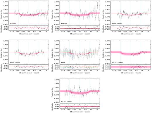
De-trended photometry from the SPECULOOS, EULER, LCO, and SAAO follow-up observations, plotted with the gp-ebop model’s transit component. The red lines and pink shaded regions show the median and the 1 and 2σ confidence intervals of gp-ebop’s posterior model.

Table 5.

Planetary properties for NGTS-4b for a circular orbit and eccentric orbit. We adopt the circular model as the most likely solution, the parameters from the eccentric model are provided for information only.

Property	Value (circular)	Value (ecc)
P (d)	1.3373508 ± 0.000008	1.3373506 ± 0.000008
TC (HJD)	2457607.9975 ± 0.0034	2457607.9978 ± 0.0033
T14 (h)	1.80 ± 0.10	1.79 ± 0.09
a/R*	4.79 ± 1.21	4.22 ± 1.18
K (m s−1)	13.7 ± 1.9	14.0 ± 2.0
e	0.0 (fixed)	|$0.14^{+0.18}_{-0.10}$|
ω (deg)	0.0 (fixed)	|$69^{+35}_{-92}$|
Mp(M⊕)	20.6 ± 3.0	20.8 ± 3.4
Rp(R⊕)	3.18 ± 0.26	3.18 ± 0.27
Rp/R*	0.035 ± 0.003	0.035 ± 0.003
ρp (g cm−3)	3.45 ± 0.95	3.50 ± 0.95
ρ* (g cm−3)	1.91 ± 0.16	1.91 ± 0.16
a (au)	0.019 ± 0.005	0.017 ± 0.004
Teq(K)	1650 ± 400	1650 ± 400
i (deg)	82.5 ± 5.8	81.0 ± 7.7

Due to the low quality of several of the follow-up light curves we also ran the global model combining the radial velocity data with just the photometry from NGTS, Callisto, Europa, and Euler-0419. The results from this run were consistent with the full model within the 1σ uncertainties (M_p=20.6 ± 3.2 M_⊕, R_p=3.25 ± 0.29 R_⊕).

In addition to the circular fit, we also present the results of the eccentric model fit in Table 5. We suspect that the fitted non-zero eccentricity in this model is due to the sparsity of RV coverage at an orbital phase of ∼0.9. Nevertheless, given that the orbit of such a short-period planet as NGTS-4b would be expected to have circularized, an eccentric orbit if true would be potentially interesting.

6 DISCUSSION

NGTS-4b is the shallowest transiting exoplanet so far discovered from the ground (see Fig. 5), with a transit depth of just 0.13 ± 0.02  per cent. It is approximately 30 per cent shallower than the second shallowest discovery – KELT-11b (Gaudi et al. 2017). The ability to be able to detect such shallow transits allows NGTS to reach down into the Neptunian desert, as evidenced by NGTS-4b, in a way that has not previously been possible for ground-based surveys. It is also encouraging for prospects of following up shallow TESS discoveries using the NGTS facility.

Figure 5.

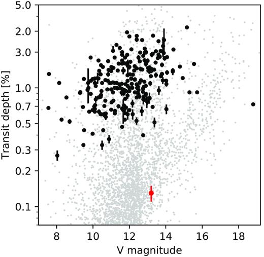
Transit depth versus host star brightness for all transiting exoplanets discovered by wide-field ground-based transit surveys. NGTS-4b is marked in red. Data from NASA Exoplanet Archive (Akeson et al. 2013) accessed on 2018 May 10. The grey dots show the simulated distribution of planet detections from TESS (Barclay, Pepper & Quintana 2018).

Fig. 6 shows the masses and radii of known transiting planets that have masses measured to better than 30 per cent, along with mass–radius relations from the models of Seager et al. (2007). The mass and radius of NGTS-4b as measured in this work are consistent with a composition of 100 per cent H₂O, however this is likely to be unphysical given the proximity to the host star, and it is more likely to consist of a rocky core with a water and/or gaseous envelope.

Figure 6.

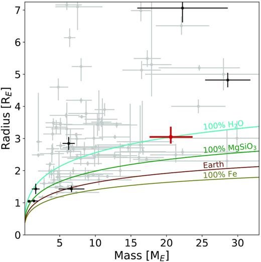
The mass and radius for all known transiting planets that have fractional errors on the measured planet mass better than 30  per cent. The black and grey points show discoveries from ground-based and space-based telescopes, respectively. The coloured lines show the theoretical mass-radius relation for solid exoplanets of various compositions (Seager et al. 2007). NGTS-4b is highlighted in red.

Studies have reported a significant dearth of Neptune-sized (R < 5 R_⊕) planets in close orbits (P<3 d), the so-called ‘Neptunian desert’ (Mazeh et al. 2016), perhaps due to the X-ray/EUV flux from the host stars quickly stripping these planets of their atmospheres and leaving them as lower mass rocky cores. However as can been seen from Fig. 7, NGTS-4b is clearly in a central region of the Neptunian desert, and is likely to still contain a significant atmosphere despite its proximity to its host star. There is nothing in our photometric or spectroscopic data to suggest that NGTS-4 is particularly young, so it is unlikely that this can explain the existence of NGTS-4b in the Neptunian desert.

Figure 7.

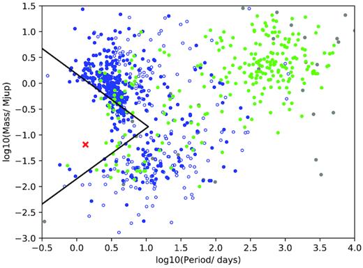
Distribution of mass versus orbital period for planets with a measured mass. Planets discovered by the transit method are shown in blue, with those having masses measured to better than 30 per cent represented as filled circles. Planets found by radial velocity are shown as green circles and those detected by other methods are shown by grey circles. Black lines represent the Neptunian desert as defined in Mazeh et al. (2016). NGTS-4b is shown as a red cross. Taken from the NASA Exoplanet Archive on 2018 August 14.

Using a typical field star age of 5 Gyr, and the X-ray-age relations of Jackson, Davis & Wheatley (2012), we estimated the X-ray luminosity of NGTS-4. This was then extrapolated to the EUV using the empirical relations determined by King et al. (2018). Scaling the combined X-ray and EUV luminosity to a flux at the planet, we followed the energy-limited approach to estimating mass loss from planetary atmospheres undergoing hydrodynamic escape (e.g. Lammer et al. 2003; Lecavelier Des Etangs 2007; King et al. 2018). Assuming a canonical evaporation efficiency of 15 per cent, we estimate a mass loss rate of 10¹⁰ g s⁻¹. This is at least an order of magnitude higher than the inferred mass loss rate of the Neptune GJ 436b, which was observed to have a 56 per cent deep transit in Lyman-alpha, corresponding to an extended comet-like tail of evaporating material (Ehrenreich et al. 2015; Lavie et al. 2017).

The X-ray luminosity of the star will have been two orders of magnitude higher during its early evolution, when it was maximally active (e.g. Jackson et al. 2012). NGTS-4b may have survived in the Neptunian desert due to an unusually high core mass (e.g. Owen & Lai 2018), or it might have migrated to its current close-in orbit after this epoch of maximum stellar activity (e.g. Jackson et al. 2012).

Future discoveries from NGTS and TESS of more Neptune-sized exoplanets should allow us to more carefully characterize the Neptunian desert and the systems that reside within it. The TESS mission (Ricker et al. 2014) is set to deliver a large number of transiting exoplanets, the bulk of which will be much shallower than can be detected from ground-based surveys (see Fig. 5). However the discovery of NGTS-4b shows that the NGTS facility is able to detect shallow transits in the magnitude range where many of the TESS candidates reside. This will be particularly important for follow-up of single-transit candidates. Villanueva, Dragomir & Gaudi (2019) estimate over 1000 single-transit candidates from TESS , of which 90 per cent will be deeper than 0.1 per cent. Such candidates will be amenable to follow-up with NGTS.

7 CONCLUSIONS

We have presented the discovery of NGTS-4b, a sub-Neptune-sized transiting exoplanet located within the Neptunian Desert. The discovery of NGTS-4b is a breakthrough for ground-based photometry, the 0.13 ± 0.02 per cent transit being the shallowest ever detected from a wide-field ground-based photometric survey. It allows us to begin to probe the Neptunian desert and find rare exoplanets that reside in this region of parameter space. In the near future, such key systems will allow us to place constraints on planet formation and evolution models and allow us to better understand the observed distribution of planets. Together with future planet detections by NGTS and TESS we will get a much clearer view on where the borders of the Neptunian desert are and how they depend on stellar parameters.

SUPPORTING INFORMATION

Table 1. Summary of NGTS photometry of NGTS-4.

Table 3. HARPS Radial Velocities for NGTS-4.

Please note: Oxford University Press is not responsible for the content or functionality of any supporting materials supplied by the authors. Any queries (other than missing material) should be directed to the corresponding author for the article.

ACKNOWLEDGEMENTS

Based on data collected under the NGTS project at the ESO La Silla Paranal Observatory. The NGTS facility is operated by the consortium institutes with support from the UK Science and Technology Facilities Council (STFC) project ST/M001962/1. This paper uses observations made at the South African Astronomical Observatory (SAAO). The contributions at the University of Warwick by PJW, RGW, DLP, DJA, BTG, and TL have been supported by STFC through consolidated grants ST/L000733/1 and ST/P000495/1. Contributions at the University of Geneva by DB, FB, BC, LM, and SU were carried out within the framework of the National Centre for Competence in Research ‘PlanetS’ supported by the Swiss National Science Foundation (SNSF). The contributions at the University of Leicester by MRG and MRB have been supported by STFC through consolidated grant ST/N000757/1. CAW acknowledges support from the STFC grant ST/P000312/1. EG gratefully acknowledges support from Winton Philanthropies in the form of a Winton Exoplanet Fellowship. JSJ acknowledges support by Fondecyt grant 1161218 and partial support by CATA-Basal (PB06, CONICYT). DJA gratefully acknowledges support from the STFC via an Ernest Rutherford Fellowship (ST/R00384X/1). PE and HR acknowledge the support of the DFG priority program SPP 1992 ‘Exploring the Diversity of Extrasolar Planets’ (RA 714/13-1). LD acknowledges support from the Gruber Foundation Fellowship. The research leading to these results has received funding from the European Research Council under the FP/2007–2013 ERC Grant Agreement number 336480 and from the ARC grant for Concerted Research Actions, financed by the Wallonia-Brussels Federation. This work was also partially supported by a grant from the Simons Foundation (PI Queloz, ID 327127). This work makes use of observations from the LCOGT network. This work has made use of data from the European Space Agency (ESA) mission Gaia (https://www.cosmos.esa.int/gaia), processed by the Gaia Data Processing and Analysis Consortium (DPAC, https://www.cosmos.esa.int/web/gaia/dpac/consortium). Funding for the DPAC has been provided by national institutions, in particular the institutions participating in the Gaia Multilateral Agreement. PyRAF is a product of the Space Telescope Science Institute, which is operated by AURA for NASA. This research has made use of the NASA Exoplanet Archive, which is operated by the California Institute of Technology, under contract with the National Aeronautics and Space Administration under the Exoplanet Exploration Program.

Footnotes

1

http://casu.ast.cam.ac.uk/surveys-projects/software-release

Author notes

Winton Fellow.