Warm dark matter chills out: constraints on the halo mass function and the free-streaming length of dark matter with eight quadruple-image strong gravitational lenses

ABSTRACT

The free-streaming length of dark matter depends on fundamental dark matter physics, and determines the abundance and concentration of dark matter haloes on sub-galactic scales. Using the image positions and flux ratios from eight quadruply imaged quasars, we constrain the free-streaming length of dark matter and the amplitude of the subhalo mass function (SHMF). We model both main deflector subhaloes and haloes along the line of sight, and account for warm dark matter free-streaming effects on the mass function and mass–concentration relation. By calibrating the scaling of the SHMF with host halo mass and redshift using a suite of simulated haloes, we infer a global normalization for the SHMF. We account for finite-size background sources, and marginalize over the mass profile of the main deflector. Parametrizing dark matter free-streaming through the half-mode mass m_hm, we constrain the thermal relic particle mass m_DM corresponding to m_hm. At |$95 \, {\rm per\, cent}$| CI: m_hm < 10^7.8 M_⊙ (⁠|$m_{\rm {DM}} \gt 5.2 \ \rm {keV}$|⁠). We disfavour |$m_{\rm {DM}} = 4.0 \,\rm {keV}$| and |$m_{\rm {DM}} = 3.0 \,\rm {keV}$| with likelihood ratios of 7:1 and 30:1, respectively, relative to the peak of the posterior distribution. Assuming cold dark matter, we constrain the projected mass in substructure between 10⁶ and 10⁹ M_⊙ near lensed images. At |$68 \, {\rm per\, cent}$| CI, we infer |$2.0{-}6.1 \times 10^{7}\, {{\rm M}_{\odot }}\,\rm {kpc^{-2}}$|⁠, corresponding to mean projected mass fraction |$\bar{f}_{\rm {sub}} = 0.035_{-0.017}^{+0.021}$|⁠. At |$95 \, {\rm per\, cent}$| CI, we obtain a lower bound on the projected mass of |$0.6 \times 10^{7} \,{{\rm M}_{\odot }}\,\rm {kpc^{-2}}$|⁠, corresponding to |$\bar{f}_{\rm {sub}} \gt 0.005$|⁠. These results agree with the predictions of cold dark matter.

gravitational lensing: strong, methods: statistical, galaxies: structure, dark matter

1 INTRODUCTION

The theory of cold dark matter (CDM) has withstood numerous tests on scales spanning individual galaxies to the large-scale structure of the Universe and the cosmic microwave background (Tegmark et al. 2004; de Blok et al. 2008; Hinshaw et al. 2013). The next frontier for this highly successful theory lies on sub-galactic scales, where CDM makes two distinct predictions: First, CDM predicts a scale-free halo mass function, possibly down to halo masses comparable to that of a planet (Hofmann, Schwarz & Stöcker 2001; Angulo et al. 2017). Second, in CDM models halo concentrations decrease monotonically with halo mass, a result of hierarchical structure formation (Moore et al. 1999; Avila-Reese et al. 2001; Zhao et al. 2003; Diemer & Joyce 2019). A confirmation of these predictions through a measurement of the mass function and halo concentrations on mass scales below 10⁹ M_⊙ would at once constitute a resounding success for CDM and rule out entire classes of alternative dark matter theories.

The abundance of small-scale dark matter depends on the matter power spectrum at early times. If the velocity distribution of the dark matter particles causes them to diffuse out of small peaks in the density field, this will prevent the direct collapse of overdensities below a characteristic scale referred to as the free-streaming length (Benson et al. 2013; Schneider, Smith & Reed 2013). The delay in structure formation in these scenarios also suppresses the central densities of the smallest collapsed haloes, changing the mass–concentration relation for low-mass objects (Avila-Reese et al. 2001; Schneider et al. 2012; Macciò et al. 2013; Bose et al. 2016; Ludlow et al. 2016). By definition, free-streaming effects are negligible in CDM, while models with cosmologically relevant free-streaming lengths are collectively referred to as warm dark matter (WDM). As the free-streaming length depends on the dark matter particle(s) mass and formation mechanism, an inference on the small-scale structure of dark matter on mass scales where some haloes are expected to be completely dark directly constrains fundamental dark matter physics and the viability of specific WDM particle candidates, including sterile neutrinos (Dodelson & Widrow 1994; Shi & Fuller 1999; Abazajian & Kusenko 2019) and keV-mass thermal relics.

Interest in alternatives to the canonical CDM paradigm, such as WDM, were motivated in part by apparent failures of the CDM model on small scales (see Bullock & Boylan-Kolchin 2017, and references therein). Two challenges in particular dominate scientific discourse, and provide illustrative examples of the complexity associated with testing CDM’s predictions on sub-galactic scales. The ‘missing satellites problem’ (MSP), first pointed out by Moore et al. (1999), refers to the paucity of observed satellite galaxies around the Milky Way, in stark contrast to dark-matter-only N-body simulations that predict hundreds of dark matter subhaloes hosting a luminous satellite galaxy. Invoking free-streaming effects in WDM to remove these small subhaloes would resolve the problem, and hence WDM models gained traction. A second challenge to the CDM picture emerged with the ‘too big to fail’ (TBTF) problem (Boylan-Kolchin, Bullock & Kaplinghat 2011), which points out that the subhaloes housing the largest Milky Way satellites are either underdense or too small. Self-interacting dark matter, which results in lower central densities in dark matter subhaloes (see Tulin & Yu 2018, and references therein), gained traction in part as a resolution to the TBTF problem.

Today, new astrophysical solutions to the MSP and TBTF problems diminish the immediate threat to CDM, but the resolutions to these issues are riddled with assumptions regarding complicated physical processes on sub-galactic scales. The inclusion of baryonic feedback and tidal stripping in N-body simulations results in the destruction of subhaloes, pushing the surviving number down to observed levels (Kim, Peter & Wittman 2017), although recently it has been suggested that the role of tidal stripping in N-body simulations is artificially exaggerated by resolution effects (van den Bosch et al. 2018; Errani & Peñarrubia 2019). The continuous discovery of new dwarf galaxies seems to resolve the MSP, and might even suggest a ‘too-many-satellites problem’ (Kim, Peter & Hargis 2018; Homma et al. 2019), but the number of expected satellite galaxies in CDM itself rests on assumptions regarding the process of star formation in low-mass haloes, which can introduce uncertainties larger than the differences between CDM and WDM on these scales (Nierenberg et al. 2016; Dooley et al. 2017; Newton et al. 2018). The inclusion of baryonic feedback from star formation processes and supernova in low-mass haloes can reduce halo central densities, and at least partially alleviates the issues associated with the TBTF problem (Tollet et al. 2016). However, the degree to which baryonic feedback resolves the problem depends on the manner in which this feedback is implemented in simulations.

Regarding constraints on WDM models, analysis of the Lyman-α forest (Viel et al. 2013; Iršič et al. 2017) and the luminosity function of distant galaxies (Menci et al. 2016; Castellano et al. 2019), while robust to the systematics associated with examining Milky Way satellites, to some degree rely on luminous matter to trace dark matter structure. Constraints from the Lyman-α forest also invokes certain assumptions for the relevant thermodynamics. The common theme is that disentangling the role of baryons and dark matter physics on sub-galactic scales is difficult and fraught with uncertainty. It would be ideal to test the predictions of matter theories irrespective of baryonic physics.

Strong gravitational lensing by galaxies provides a means of testing the predictions of dark matter theories directly, without relying on baryons to trace the dark matter. As photons emitted from distant background sources traverse the cosmos, they are subject to deflections by the gravitational potential of dark matter haloes along the entire line of sight and by subhaloes around the main lensing galaxy. Each warped image produced by a strong lens contains a wealth of information regarding the dark matter structure in the Universe. The aim of this work is to extract that information.

When the lensed background source is spatially extended – for example, a galaxy – the lensed image becomes an arc that partially encircles the main deflector. Dark matter haloes near the arc produce small surface brightness distortions, which allows for the localization of the perturbing halo and enables constraints on its mass down to scales somewhere between 10⁸ and 10⁹ M_⊙ (Vegetti et al. 2014; Hezaveh et al. 2016b). Analysis of the surface brightness fluctuations over the entirety of the arc can also constrain the abundance of small haloes too diminutive to be detected individually, and results in a 2 keV lower bound on the mass of thermal relic WDM (Birrer, Amara & Refregier 2017b). A joint analysis of individual detections and non-detections in a sample of arc-lenses can constrain certain models of dark matter and test the predictions of CDM (Vegetti et al. 2018; Ritondale et al. 2019). Recently, several works have proposed measuring the substructure convergence power spectrum by analysing surface brightness fluctuations in extended arcs (Hezaveh et al. 2016a; Díaz Rivero et al. 2018; Brennan et al. 2019; Cyr-Racine, Keeton & Moustakas 2019), and Bayer et al. (2018) applied this method to a strong lens system.

We focus on a second kind of lens system, quadruply imaged quasars (quads). Rather than extended arcs, the observables in quads are four image positions and three magnification ratios, or flux ratios (the observable is the flux ratio, not the intrinsic flux, because the intrinsic source brightness is unknown) with unresolved sources. Flux ratios depend on non-linear combinations of second derivatives of the lensing potential near an image, providing localized probes of small-scale structure down to scales of 10⁷ M_⊙. These systems have been used in the past to constrain the presence of dark matter haloes near lensed images (Metcalf & Madau 2001; Metcalf & Zhao 2002; Amara et al. 2006; Nierenberg et al. 2014, 2017) and measure the subhalo mass function (SHMF; Dalal & Kochanek 2002, hereafter DK2). Recently, Hsueh et al. (2019, hereafter H19) improved on previous analyses of quadruply imaged quasars by including haloes along the line of sight, which can contribute a significant signal in flux ratio perturbations (Xu et al. 2012; Gilman et al. 2018). They found results consistent with CDM, ruling out WDM models to a degree comparable to that of the Lyman-α forest (Viel et al. 2013; Iršič et al. 2017).

In the case of quadruple-image lenses, the luminous source is often a compact background object, such as the ionized medium around a background quasar. Broad-line emission from the accretion disc is subject to microlensing by stars, whereas light that scatters off of the more spatially extended narrow-line region is immune to microlensing while retaining sensitivity to the milliarcsecond scale deflection angles produced by dark matter haloes in the range 10⁷–10¹⁰ M_⊙ (Moustakas & Metcalf 2003; Sugai et al. 2007; Nierenberg et al. 2014, 2017). Likewise, radio emission from the background quasar, while generally expected to be more compact than the narrow-line emission based on certain quasar models (Elitzur & Shlosman 2006; Combes et al. 2019), is extended enough to absorb micro-lensing effects.

We carry out an analysis of eight quads using a forward-modelling approach we have tested and verified with mock data sets (Gilman et al. 2018, 2019). The sample of lenses we consider contains six systems with flux ratios measured with narrow-line emission presented in Nierenberg et al. (2019), and two others with data from Nierenberg et al. (2014, 2017). We expect the sample is robust to microlensing effects and yield reliable data with which to constrain dark matter models. None of the quads show evidence for morphological complexity in the form of stellar discs, which require more detailed lens modelling (Hsueh et al. 2016; Gilman et al. 2017; Hsueh et al. 2017).

This paper is organized as follows: In Section 2, we describe our forward-modelling analysis method and our implementation of a rejection algorithm in Approximate Bayesian Computing. Section 3 describes our parametrizations for the dark matter structure in the main lens plane and along the line of sight, and our modelling of free-streaming effects in WDM. Section 4 contains a brief description of the data used in our analysis and the relevant references for each system. In Section 5, we describe in detail each physical assumption we make and the modelling choices and prior probabilities attached to these assumptions. In Section 6, we present our inferences on the free-streaming length of dark matter and the amount of lens plane substructure. We discuss the implications of our results and our general conclusions in Section 7.

All lensing computations are performed using lenstronomy¹ (Birrer & Amara 2018). Cosmological computations involving the halo mass function and the matter power spectrum are performed with colossus (Diemer 2018). We assume a standard cosmology using the parameters from WMAP9 (Hinshaw et al. 2013) (Ω_m = 0.28, σ₈ = 0.82, h = 0.7).

2 BAYESIAN INFERENCE IN SUBSTRUCTURE LENSING

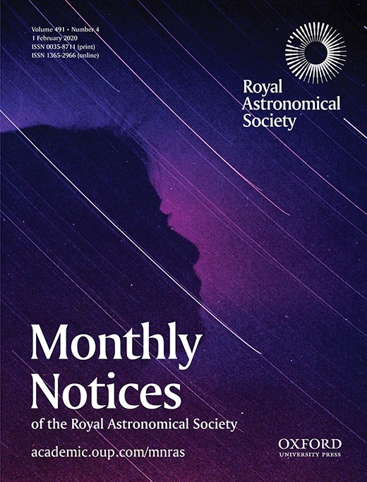
In this section, we frame the substructure lensing problem in a Bayesian context, and describe our analysis method which relies on a forward-generative model to sample the target posterior distribution through an implementation of Approximate Bayesian Computing. We have tested this analysis method using simulated data (Gilman et al. 2018, 2019). The full forward-modelling procedure we describe in this section is illustrated in Fig. 1, and the relevant parameters are summarized in Table 1.

Figure 1.

A graphical representation of the forward-modelling procedure. The purple colours correspond to the action of sampling from a prior, blue represents an operation performed using the parameters sampled from a prior, and the green colours indicate the use of observed information from the lenses. The arrow of time points from top to bottom: The first step is the rendering of dark matter structure, while the use of the information from observed flux ratios happens only at the very end.

Table 1.

Free parameters sampled in the forward model. Notation |$\mathcal {N} (\mu , \sigma)$| indicates a Gaussian prior with mean μ and variance σ, and |$\mathcal {U} (u_1, u_2)$| indicates a uniform prior between u₁ and u₂. Lens-specific priors are summarized in Table 2.

Parameter	Definition	Prior
log10(Mhalo)[M⊙]	main lens parent halo mass	(lens specific)
|$\Sigma _{\rm {sub}} [\rm {kpc}^{-2}]$|	normalization of SHMF (equation 7)	|$\mathcal {U} (0, 0.1)$|
	(rendered between 106 and 1010 M⊙)
α	logarithmic slope of the SHMF	|$\mathcal {U} (-1.95, -1.85)$|
log10(mhm)[M⊙]	half-mode mass (equations 11 and 12)	|$\mathcal {U} (4.8, 10)$|
	∝ to free-streaming length and thermal relic mass mDM
δlos	rescaling factor for the line of sight Sheth–Tormen	|$\mathcal {U} (0.8, 1.2)$|
	mass function (equation 9), rendered between 106 and 1010 M⊙)
|$\sigma _{\rm {src}} [\rm {pc}]$|	source size	|$\mathcal {U} (25, 60)$|
	parametrized as FWHM of a Gaussian
γmacro	logarithmic slope of main deflector mass model	|$\mathcal {U} (1.95, 2.2)$|
γext	external shear in the main lens plane	(lens specific)
|$\delta _{xy} [\rm {m.a.s.}]$|	image position uncertainties	(lens specific)
δf	image flux uncertainties	(lens specific)

2.1 The Bayesian inference problem

Our goal is to obtain samples from the posterior distribution

$$\begin{eqnarray*} p ({{\bf q}_{\rm {s}}}| \boldsymbol{D}) \propto \pi ({{\bf q}_{\rm {s}}}) \prod _{n=1}^{N} \mathcal {L} ({{\bf d}_{\rm {n}}}| {{\bf q}_{\rm {s}}}), \end{eqnarray*}$$

(1)

where q_s is a set of hyper-parameters describing the subhalo and line-of-sight halo mass functions, |$\boldsymbol{D}$| denotes the set of positions and flux ratios from a set of N lenses with the data from each lens denoted by d_n, and where π represents the prior on q_s.

A certain dark matter model makes predictions for the parameters in q_s, which includes quantities such as the normalization of the SHMF, the logarithmic slope of the mass function, a free-streaming cut-off, etc. For a given q_s, we may generate specific realizations of line-of-sight haloes and main deflector subhaloes (including the halo/subhalo masses, positions, concentrations, etc.), which affect lensing observables. We refer to a specific realization of dark matter structure corresponding to a model specified by q_s as m_sub. In addition to generating the realizations m_sub, computing the likelihood function |$\mathcal {L} ({{\bf d}_{\rm {n}}}| {{\bf q}_{\rm {s}}})$| in equation (1) requires marginalizing over nuisance parameters M, which include the background source size σ_src, and the lens model that describes the main lensing galaxy (hereafter the macromodel). Integrating over the macromodel and the space of possible dark matter realizations m_sub, the likelihood is given by

$$\begin{eqnarray*} \mathcal {L} ({{\bf d}_{\rm {n}}}| {{\bf q}_{\rm {s}}}) = \int p ({{\bf d}_{\rm {n}}}| {{\bf m}_{\rm {sub}}}, {}{{\bf M}}) p ({{\bf m}_{\rm {sub}}}, {}{{\bf M}}| \ {{\bf q}_{\rm {s}}}) \mathrm{ d} {{\bf m}_{\rm {sub}}}\ \mathrm{ d} {}{{\bf M}}. \end{eqnarray*}$$

(2)

Note that we write the joint distribution p(m_sub, M|q_s), and do not assume the parameters in M and q_s are independent.

Evaluating equation (2) is a daunting task. We highlight two main reasons:

• Exploring the parameter space spanned by q_s and M through traditional MCMC methods is extremely inefficient. M is a high-dimensional space, where the overwhelming majority of volume does not result in model-predicted observables that resemble the data, and in particular does not predict the correct image positions. Thus, the overwhelming majority of samples drawn from M, and the corresponding samples q_s (even if they described the ‘true’ nature of dark matter) would not contribute to the integral.

• The parameters M describing the lens macromodel may depend indirectly on the dark matter parameters q_s through the realizations m_sub generated from the model specified by q_s. This necessitates the simultaneous sampling of q_s and M in the inference. However, it is difficult to impose an informative prior on M since the ‘true’ parameters in q_s are unknown. Recognizing this and using a very uninformative prior on M, most samples will be rejected since they do not resemble the data, which alludes back to the issue of dimensionality described in the first bullet point.

To address these challenges, we use a statistical method that bypasses the direct computation of the integral in equation (2).

2.2 Forward modelling the data

Rather than compute the likelihood function, we recognize that by creating simulated observables |${{\bf d}_{\rm {n}}^{\prime }}= {{\bf d}_{\rm {n}}^{\prime }}({{\bf m}_{\rm {sub}}}, {}{{\bf M}})$| from the model q_s, and accepting the proposed q_s if they satisfy |${{\bf d}_{\rm {n}}^{\prime }}= {{\bf d}_{\rm {n}}}$|⁠, the accepted q_s samples will be direct draws from the posterior distribution in equation (1) (Rubin 1984). In this forward-generative framework, simulating the relevant physics in substructure lensing replaces the task of evaluating the likelihood function in equation (2). We propagate photons from a finite-size background source through lines of sight populated by dark matter haloes, a lensing galaxy and its subhaloes, and finally into a simulated observation with statistical measurement errors added. Provided the forward model contains all of the relevant physics, the simulated data |${{\bf d}_{\rm {n}}^{\prime }}$| will express the same potentially complex covariances present in the observed data.

The ‘curse of dimensionality’ that prohibits direct evaluation of equation (2) also afflicts the criterion of exact matching between d_n and |${{\bf d}_{\rm {n}}^{\prime }}$|⁠. In particular, most draws of macromodel parameters M will not yield the observed image positions, and would therefore be rejected from the posterior. To deal with this, our strategy will be to ensure that the macromodel and other nuisance parameters sampled in the forward model, when combined with the full line of sight and subhalo populations specified by m_sub, yield a lens model that predicts the same image positions as observed in the data.

Obtaining a lens model that returns the observed image positions amounts to demanding that the four images seen by the observer on the sky at positions |$\boldsymbol{\theta }$| map to the same position on the source plane |$\boldsymbol{\beta _K}$|⁠. This requires the use of the full multiplane lens equation describing the path of deflected light rays (e.g. Schneider 1997, see also Blandford & Narayan 1986)

$$\begin{eqnarray*} \boldsymbol{\beta _K} = \boldsymbol{\theta } - \frac{1}{D_{\rm {s}}} \sum _{k=1}^{K-1} D_{\rm {ks}}{\boldsymbol{\alpha _{\rm {k}}}} (D_{\rm {k}} \boldsymbol{\beta _{\rm {k}}}), \end{eqnarray*}$$

(3)

where the quantities D_s, D_k and D_ks denote angular diameter distances to the source plane, to the kth lens plane, and from the kth lens plane to the source plane, respectively. Equation (3) is a recursive equation for the |$\boldsymbol{\beta _{\rm {k}}}$| that couples deflection angles from objects at different redshifts, similar to looking through potentially thousands of magnifying glasses in series. Throughout this process, we account for uncertainties in the measured image positions by sampling astrometric perturbations δ_xy, and applying them to the observed image positions during the forward modelling.

To solve for macromodel parameters M, for each realization m_sub we sample the power-law slope of the main deflector mass profile γ_macro and the external shear strength γ_ext. If the lens system in question has satellite galaxies or nearby deflectors, we sample priors for their masses and positions. The remaining parameters describing the lens macromodel² are allowed to vary freely until a lens model that fits the image positions is found.³

The approach of simultaneously sampling M and q_s does not involve lens model optimizations with respect to the observed image fluxes, because the information from the observed fluxes is not used at this stage of the analysis. This method therefore avoids potential biases incurred by optimizing the macromodel with respect to the observed fluxes, rather than marginalizing over these parameters. As we will show in Section 6.1, by sampling M and q_s simultaneously we obtain joint posterior distributions that account for potential covariance between these quantities, recognizing that the addition of substructure may affect the distributions for the macromodel parameters in M.

With a lens model that fits the image positions in hand, we draw a background source size and ray-trace on a finely sampled grid around each image position using equation (3) to compute the image fluxes |$\boldsymbol{f^{\prime }}$|⁠. To incorporate statistical measurement errors in image fluxes, we sample flux uncertainties |$\boldsymbol{\delta f}$|⁠, and render these perturbations on to the model-predicted fluxes |$\boldsymbol{f^{\prime }} \rightarrow \boldsymbol{f^{\prime }} + \boldsymbol{\delta f}$| prior to computing the flux ratios.

2.3 Deriving posteriors from the forward model samples

For each realization, we compute a summary statistic between the three observed flux ratios |$\boldsymbol{f_{\rm {obs}}}$| and those computed in the forward model

$$\begin{eqnarray*} S_{\rm {lens}} (\boldsymbol{f^{\prime }},\boldsymbol{f_{\rm {obs}}}) \equiv \sqrt{\sum _{i=1}^{3} \left({f}^{\prime }_{i} - f_{\rm {obs(i)}} \right)^2}, \end{eqnarray*}$$

(4)

and assign this statistic to the draw of q_s. This summary statistic contains the full information content of the data, as the simultaneous matching of the three ratios requires that the forward model samples that minimize this statistic contain the same correlations present in the data. We repeat this procedure between 300 000 and 1200 000 times for each quad, depending on the frequency with which the realizations, with the statistical flux uncertainties added, match the observed fluxes to within |$1\, {\rm per\, cent}$|⁠.

We select the q_s parameters corresponding to the 800 lowest summary statistics S_lens. The exact matching criterion |${{\bf d}_{\rm {n}}}= {{\bf d}_{\rm {n}}^{\prime }}$|⁠, which guarantees that the accepted samples q_s form the desired posterior, is replaced by selecting the realizations that look most like the data through the summary statistic S_lens. The resulting distribution of q_s is therefore an approximation to the posterior distribution for each lens, with the approximation converging to the true posterior as the number of forward model samples increases while keeping the number of accepted samples fixed. The quality of the approximation can be quantified through a convergence test, in which we verify that the posteriors are unchanged as one removes realizations from the forward-modelled data while keeping the same number of accepted samples (see Appendix  A). This method is an implementation of a rejection algorithm in Approximate Bayesian Computing (Rubin 1984; Marin et al. 2011; Lintusaari et al. 2017), a technique applied to problems where it is possible to generate simulated data from the model, but difficult to compute the likelihood (see also Beaumont, Zhang & Balding 2002; Akeret et al. 2015; Birrer, Amara & Refregier 2017b; Hahn et al. 2017).

To obtain the final posterior distribution |$p ({{\bf q}_{\rm {s}}}| \boldsymbol{D})$| (equation 1), we multiply together the likelihoods obtained for each lens.⁴ This procedure is only possible when using uniform priors in the forward model sampling, as the use of non-uniform priors would effectively move π(q_s) inside the product in equation (1) and overuse this information. We may, however, impose any prior we wish a posteriori by re-weighting the forward model samples accordingly.

3 THE SUBHALO AND LINE-OF-SIGHT HALO POPULATIONS

In this section, we describe the models we implement for the line of sight and SHMFs in cold and warm dark matter that we sample in the forward model. We also describe the density profiles for individual haloes, including their truncation radii and their distribution both along the line of sight and in the main lens plane. We begin with the parametrizations used for the halo and subhalo density profiles and the spatial distribution of subhaloes in Section 3.1. In Sections 3.2 and 3.3, we describe the parametrizations of the subhalo and line-of-sight halo functions, respectively, and in Section 3.4 describe how we model WDM free-streaming effects.

3.1 Subhalo density profiles and spatial distribution

We model subhaloes as tidally truncated NFW profiles (Baltz, Marshall & Oguri 2009)

$$\begin{eqnarray*} \rho (r) = \frac{\rho _s}{x (1+x)^2} \frac{\tau ^2}{x^2 + \tau ^2}, \end{eqnarray*}$$

(5)

where |$x = \frac{r}{r_\mathrm{ s}}$|⁠, |$\tau = \frac{r_\mathrm{ t}}{r_\mathrm{ s}}$|⁠, and r_t is a truncation radius and r_s is the NFW profile scale radius. We use the mass definition of M₂₀₀ computed with respect to the critical density at z = 0, and a concentration–mass relation that accounts for free-streaming effects in WDM as is specifically designed to accurately predict the concentrations of low-mass haloes (see Section 3.4).

In the main lens plane, we truncate haloes according to their three-dimensional position inside the host halo r_3D through a Roche-limit approximation that assumes a roughly isothermal global mass profile. The relevant scaling is |$r_\mathrm{ t} \propto (M_{200} r_{\rm {3D}}^{2})^{\frac{1}{3}}$| (Tormen, Diaferio & Syer 1998; Cyr-Racine et al. 2016), which we implement as

$$\begin{eqnarray*} r_\mathrm{ t} = 1.4 \left(\frac{M_{200}}{10^7\, {{\rm M}_{\odot }}}\right)^{\frac{1}{3}} \left(\frac{r_{\rm {3D}}}{50 \,\rm {kpc}}\right)^{\frac{2}{3}} [\rm {kpc}]. \end{eqnarray*}$$

(6)

This results in truncation radii of ∼4–10r_s. We note that the truncation radius depends implicitly on the host halo mass M_halo through r_3D, which depends on the scale radius and the virial radius of the host halo at the lens redshift (see Fig. 4). We note that the definition of r_t in equation (6) does not depend on the structural parameters of the subhalo, which are altered in WDM models (see Section 3.4). Incorporating these modelling details requires prescriptions for the tidal evolution of subhaloes in the host halo as a function of the physical properties of the subhalo at infall (e.g. Green & van den Bosch 2019).

We render subhaloes out to a maximum projected radius 3R_Ein and assign a three-dimensional z-coordinate between −r₂₀₀ and r₂₀₀, where r₂₀₀ is the virial radius of the host. Inside this volume, we distribute the subhaloes assuming the spatial distribution follows the mass profile of the host dark matter halo outside an inner tidal radius, which we fix to half the scale radius of the host. Inside this radius, we distribute subhaloes with a uniform distribution in three dimensions. This choice is motivated by simulations that predict tidal disruption of subhaloes near the lensing galaxy, resulting in an approximately uniform number of subhaloes per unit volume in the inner regions of the halo (Jiang & van den Bosch 2017). The spatial distribution of subhaloes that results from this procedure is approximately uniform in projection, which agrees with the predictions from N-body simulations (Xu et al. 2015).

3.2 The CDM subhalo mass function

In principle, the projected mass in subhaloes near the Einstein radius can depend on the host halo mass, redshift, and the severity of tidal stripping by the main lensing galaxy. We will ultimately combine the inferences from multiple lenses at different redshifts and with different host halo masses, so we parametrize the SHMF in such a way that a single parameter Σ_sub can be used to simultaneously describe the projected mass density in substructure for each quad, regardless of halo mass or redshift.

We use the functional form for the SHMF

$$\begin{eqnarray*} \frac{\mathrm{ d}^2 N_{\rm {sub}}}{\mathrm{ d}m \mathrm{ d}A} = \frac{\Sigma _{\rm {sub}}}{m_0} \left(\frac{m}{m_0}\right)^{\alpha } \mathcal {F} (M_{\rm {halo}}, z), \end{eqnarray*}$$

(7)

where scaling function |$\mathcal {F} (M_{\rm {halo}}, z)$| encodes the differential evolution of the projected number density with redshift and host halo mass, such that Σ_sub can be interpreted as a common parameter for all the lenses. We choose the normalization such that |$\mathcal {F} (M_{\rm {halo}} = 10^{13} {{\rm M}_{\odot }}, z = 0.5) = 1$|⁠, anchoring Σ_sub at z = 0.5 with a halo mass of 10¹³ M_⊙. We use a pivot mass m₀ = 10⁸ M_⊙. We will marginalize over Σ_sub and α when quoting constraints on dark matter warmth to account for tidal stripping of subhaloes and halo-to-halo scatter.

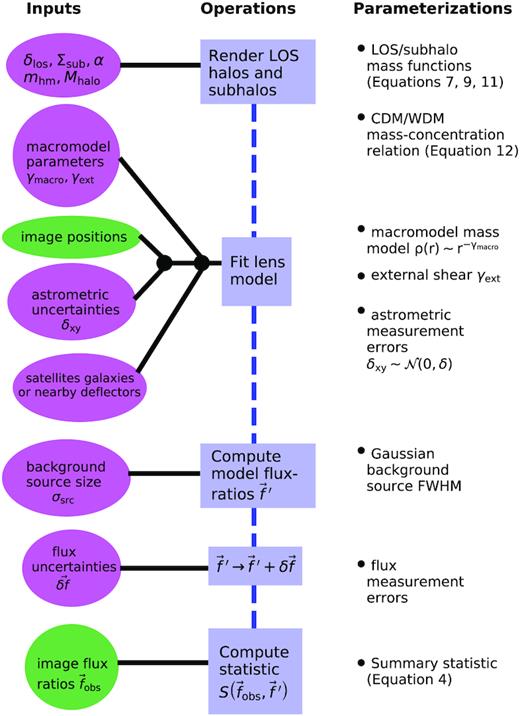
To determine the scaling function |$\mathcal {F} (M_{\rm {halo}}, z)$|⁠, we run a suite of simulations using the semi-analytic modelling code galacticus⁵ (Benson 2012; Pullen, Benson & Moustakas 2014), simulating host haloes and their substructure in the redshift range 0.2 < z < 0.8 and mass range 0.8–3 × 10¹³ M_⊙, with a subhalo mass resolution of 10⁸ M_⊙. In each redshift and mass bin we simulate 24 haloes, resulting in 840 haloes with M_halo ∼ 10¹³ M_⊙ in total.⁶ We average over the projected number densities along each principle axis inside a 15 kpc aperture to obtain trends in the projected number density with host halo mass and redshift in the vicinity of the Einstein radius, where lensed images appear. The galacticus simulations include tidal destruction of subhaloes by the global dark matter mass profile, which affects the evolution of the projected mass density with host halo redshift: at early times, subhaloes are more concentrated in the host, while at later times tidal stripping from the host depletes the population of subhaloes at small radii and the projected number density near the Einstein radius decreases. In addition, the physical size of the host halo at higher redshifts is smaller by a factor of (1 + z)⁻¹, so the number of subhaloes per square physical kpc is higher. We also note that early-type galaxy host haloes simulated by Fiacconi et al. (2016) also show significant evolution with redshift in the projected number density of subhaloes by about a factor of two, very similar to the galacticus predictions.

We fit the evolution with halo mass and redshift predicted by galacticus with the relation

$$\begin{eqnarray*} \log _{10} (\mathcal {F}) = k_1 \log _{10} \left(\frac{M_{\rm {halo}}}{10^{13}\, {{\rm M}_{\odot }}}\right) + k_2 \log _{10}(z+0.5) \end{eqnarray*}$$

(8)

with k₁ = 0.88 and k₂ = 1.7. The galacticus output and the fit from equation (8) are shown in Fig. 2. We only extract information regarding the scaling of projected mass density with halo mass and redshift from the galacticus simulations, and treat the overall normalization of the number density as a free-parameter that absorbs the effects of tidal destruction of subhaloes by the main lens galaxy. We discuss our modelling assumptions in more detail in Section 5.4.

Figure 2.

Output from the galacticus semi-analytic simulations of substructure within haloes used to calibrate the evolution of the SHMF with halo mass and redshift. While on the y-axis we plot the actual projected surface mass density in substructure output by galacticus, we only use the scaling with halo mass in redshift in our modelling, treating the overall normalization of the SHMF as a free parameter. The projected mass density in substructure on the y-axis corresponds to a mass range 10⁶–10¹⁰ M_⊙, where we have extrapolated the mass function from the smallest resolved subhalo (10⁸ M_⊙) to 10⁶ M_⊙ to compute the projected mass.

3.3 The line-of-sight halo mass function

We model line-of-sight structure by drawing halo masses from the Sheth–Tormen halo mass function (Sheth, Mo & Tormen 2001), with two modifications. First, we introduce an overall rescaling factor δ_los which accounts for theoretical uncertainty in the predicted amplitude of the halo mass function (see e.g. Despali et al. 2016). The factor δ_los accounts for the possibility of a selection bias in the quads towards systematically overdense or underdense lines of sight. The second modification we add is a contribution from the two-halo term ξ_2halo(M_halo, z), which accounts for the presence of correlated structure in the vicinity of main deflector parent dark matter halo.⁷ With these modifications the line-of-sight halo mass function takes the form

$$\begin{eqnarray*} \frac{\mathrm{ d}^2N_{\rm {los}}}{\mathrm{ d}m \mathrm{ d}V} = {\delta _{\rm {los}}}(1+ \xi _{\rm {2halo}}(M_{\rm {halo}}, z)) \frac{\mathrm{ d}^2N}{\mathrm{ d}m \mathrm{ d}V} \big \vert _{\rm {ShethTormen}}. \end{eqnarray*}$$

(9)

Haloes along the line of sight are rendered in a double-cone geometry with opening angle 3R_Ein, where R_Ein is the Einstein radius of the main deflector, and a closing angle behind the main deflector such that the cone closes at the source redshift. Finally, we add negative convergence sheets to subtract the mean expected convergence from line-of-sight haloes at each line of sight plane. Without this numerical procedure, lines of sight are systematically overdense relative to the expected matter density of the Universe, akin to lensing in a universe with positive curvature (Birrer et al. 2017a). This may bias results as the macromodel will attempt to compensate for the artificial focusing of light rays in this scenario.

3.4 Modelling free-streaming effects in WDM

Free-streaming refers to the diffusion of dark matter particles out of small peaks in the matter density field in the early Universe. This has the effect of erasing structure on scales below a characteristic free-streaming length which depends on the velocity distribution of the dark matter particles, and hence on their mass and formation mechanism. For a more in-depth discussion, see Schneider et al. (2013).

It is convenient to express free-streaming effects in terms of the half-mode mass m_hm, which is defined in terms of the length-scale where the transfer function between the CDM and WDM power spectra drops to one-half. In the specific case that all of the dark matter exists in the form of thermal relics, a one-to-one mapping between the half-mode mass and the mass of the candidate particle m_DM exists, and has the scaling |${m_{\rm {hm}}}\propto m_{\rm {DM}}^{-3.33}$| (Schneider et al. 2012)

$$\begin{eqnarray*} m_{\rm {hm}}(m_{\rm {DM}}) = 3\times 10^{8} \left(\frac{m_{\rm {DM}}}{\rm {3.3\,keV}}\right)^{-3.33} {{\rm M}_{\odot }}. \end{eqnarray*}$$

(10)

We have run galacticus models (Benson et al. 2013) with WDM mass functions corresponding to 3.3 and 5 keV thermal relics to investigate the effects of free-streaming on the trends with host halo mass and redshift of the projected mass in substructure near the Einstein radius, and determine that the fit in equation (8) is common to both CDM and WDM. We therefore use the same scaling function |$\mathcal {F} (M_{\rm {halo}}, z)$| for WDM SHMFs, and model the effects of free-streaming using the fitting formula from Lovell et al. (2014)

$$\begin{eqnarray*} \frac{\mathrm{ d}N_{\rm {WDM}}}{\mathrm{ d}m} = \frac{\mathrm{ d}N_{\rm {CDM}}}{\mathrm{ d}m} \left(1+\frac{m_{\rm {hm}}}{m} \right)^{-1.3}. \end{eqnarray*}$$

(11)

Since the parameter m_hm is related to the WDM transfer function, it should affect the subhalo and field halo mass functions in a similar manner. We therefore apply the same suppression factor in equation (11) to both the SHMF and the line-of-sight halo mass function in equations (7) and (9), respectively. Lacking a theoretical prediction for the evolution of the turnover with redshift, we do not evolve the shape or position of the free-streaming cut-off in the mass function at higher redshifts.

In WDM scenarios, the delayed onset of structure formation affects the assembly history of dark matter haloes and suppresses their concentrations |$c \equiv \frac{r_{\rm {vir}}}{r_\mathrm{ s}}$|⁸ on mass scales that extend above m_hm (Schneider et al. 2012; Bose et al. 2016). We use the functional form proposed by Bose et al. (2016), and write the WDM concentration–mass relation as

$$\begin{eqnarray*} \frac{c_{\rm {WDM}}(m, z)}{c_{\rm {CDM}}(m, z)} = (1+z) ^{\beta (z)} \left(1+60\frac{m_{\rm {hm}}}{m}\right)^{-0.17} \end{eqnarray*}$$

(12)

with β(z) = 0.026z − 0.04, using the CDM mass–concentration model of Diemer & Joyce (2019) and a scatter of 0.1 dex (Dutton & Macciò 2014). The WDM suppression factor for the mass–concentration relation we use was calibrated for haloes on mass scales below M₂₀₀ ∼ 10⁹ M_⊙, and is accurate in the redshift range z = 0–3. We note that since flux ratios are particularly sensitive to the central density of perturbing haloes, the suppression of halo concentrations far above m_hm (because of the factor of 60 in equation 12) is possibly the dominant effect of dark matter free-streaming on lensing observables. We plot the SHMF and the halo mass–concentration–redshift relation in Fig. 3.

Figure 3.

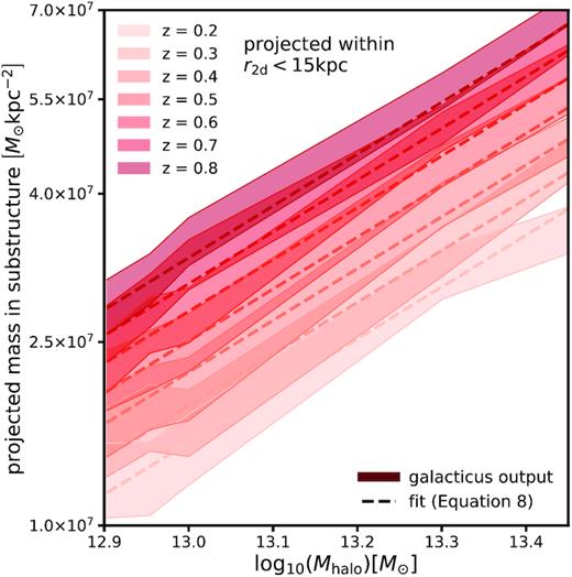
Top: The SHMF as a function of halo mass, redshift, and the half-mode mass m_hm = 10⁷ M_⊙ with |$\Sigma _{\rm {sub}} = 0.012 \,\rm {kpc^{-2}}$|⁠. The line-of-sight halo mass function looks similar, but evolves differently with redshift. Bottom: The mass–concentration relation for CDM and the same WDM model with m_hm = 10⁷ M_⊙. Free-streaming affects the concentration of haloes over one order of magnitude above m_hm.

4 THE DATA

We apply the forward-modelling methodology outlined in Section 2 using the physical model described in Section 3 to eight quadruply imaged quasars. In this section, we describe the sample selection, and how the data for these eight systems were obtained. In Table C1 in Appendix  C, we summarize the data used in the analysis and provide the relevant references.

4.1 The narrow-line systems

The quads in our sample have image fluxes measured using the narrow-line emission from the background quasar. Six of these (WGD 2038, WFI 2033, RX J0911, PS J1606, WGD J0405, and WFI 2026) have flux and astrometry presented by Nierenberg et al. (2019), while the data for B1422 and HE0435 are taken from Nierenberg et al. (2014) and Nierenberg et al. (2017), respectively. The flux uncertainties for the narrow-line lenses are estimated from the forward-modelling method used to fit the narrow-line spectra. For additional details regarding the measurement methodology for the narrow-line flux ratios, we refer to Nierenberg et al. (2017, 2019).

Shajib et al. (2019) analysed several systems in our sample. They measured satellite galaxy location and provided the photometric information for the systems J1606 and WGD J0405, which we used to obtain photometric redshifts (see Appendix  B).

4.2 Lenses omitted from our sample

We apply our analysis to a sample of eight quads, although additional systems exist in the literature with measured flux ratios. We choose only a subset of the total number of possible lenses since the remaining systems either do not have reliable flux measurements, or have complicated deflector morphology that introduces significant uncertainties in the lens modelling. We do not include lenses with fluxes measured using radio emission from the background quasar. Some of these systems may be analysed in a future work upon revision of our modelling strategy and new flux measurements.

Specifically, we do not include quads with main lensing galaxies that contain stellar discs, since accurate lens models for these systems require explicit modelling of the disc. This excludes the system J1330 presented by Nierenberg et al. (2019). We also exclude HS 0810, a system with narrow-line flux measurements presented by Nierenberg et al. (2019), because the flux from the merging images becomes blended together for source sizes larger than 20 pc. This complicates our analysis, as our method for computing image fluxes with extended background sources cannot be applied to merging pairs when the images blur together.

5 PHYSICAL ASSUMPTIONS AND PRIORS

The parametrizations we introduce in Section 3 and the priors use in the forward model reflect certain physical assumptions. In this section, we describe these assumptions, and the prior probabilities attached to each parameter in the forward model for our sample of quads.

5.1 The extended background source

The effect of a dark matter halo of a given mass on the magnification of a lensed image is a function of the background source size (Dobler & Keeton 2006), see also fig. 14 in Amara et al. (2006) and fig. 8 in Xu et al. (2012). In general, more extended background sources are less sensitive to dark matter haloes (in terms of the image magnifications) on the mass scales relevant for substructure lensing, and the minimum sensitivity threshold for a halo of a given max to produce a measurable flux perturbation is determined by the background source size.

The lenses in our sample have fluxes measured using emission from the narrow-line region of the background quasar (Nierenberg et al. 2017, 2019). The narrow-line region is expected to subtend angular scales larger than a micro-arcsecond, corresponding to physical scales larger than |${\sim}1 \,\rm {pc}$|⁠, such that it is immune to microlensing by stars. This physical extent also corresponds to a light-crossing time greater than the typical time delay between lensed images, such that variability in the background quasar should be washed out of the light curves if the source size is indeed large enough to avoid microlensing.

The size of the narrow-line region typically spans up to |${\sim}60 \,\rm {pc}$| (Müller-Sánchez et al. 2011) defined as the full width at half-maximum (FWHM) of the radially averaged luminosity profile. Upper limits of 50–60 pc may also be obtained by forward modelling the spectrum of the lensed images themselves (Nierenberg et al. 2017). We therefore model the background source as a circular Gaussian and impose a uniform prior on the FWHM between |$25\,\,\mathrm{ and}\,\,{-}60 \,\rm {pc}$|⁠.

5.2 Halo and subhalo mass ranges

We render haloes for both the line of sight and SHMFs in the range 10⁶–10¹⁰ M_⊙. Haloes with masses below 10⁶ M_⊙ do not leave imprints on lensing observables for the extended source sizes we consider, which we verify by comparing distributions of image flux ratios with different minimum subhalo masses. The smallest halo masses flux ratios are sensitive to depend on the background source size and the concentration of the halo, but we estimate through ray-tracing simulations that the lower limit lies somewhere between 10⁶ and 10⁷ M_⊙ for the smallest source sizes we model. We include the rare objects more massive than 10¹⁰ M_⊙ by explicitly including them in the lens model, assuming that they host a luminous galaxy, in which case they are detected in the observations of the lenses themselves. This assumption is consistent with current abundance matching techniques (Kim et al. 2018; Nadler et al. 2019).

5.3 The line-of-sight halo mass function

We use the Sheth–Tormen (Sheth et al. 2001) halo mass function to model structure along the line of sight, with two modifications: First, we introduce a rescaling term δ_los to account for a systematic shift in the predicted mean amplitude of the mass function. Second, we include a term ξ_2halo(M_halo, z) that rescales the amplitude of the mass function near the main deflector to account for the presence of correlated structure in the density field near the parent dark matter halo. This results in a |$5{-}10 \, {\rm per\, cent}$| increase in the number haloes near the main deflector.

Apart from uncertainty in the overall amplitude δ_los, we assume the halo mass function in the lens cone volume is well described by the mean halo mass function in the Universe. This is a reasonable approximation as lensing volumes span several Gpc, and we expect fluctuations in the dark matter density along the line of sight should average out over large distances. We note, however, that there is some scatter among the predictions from different parametrizations of the halo mass function below 10¹⁰ M_⊙ (e.g. Despali et al. 2016) and cosmological model uncertainties, for instance associated with σ₈ and Ω_m. It is also possible that lenses are selected preferentially in overdense or underdense lines of sight. We use a flat prior on δ_los between 0.8 and 1.2 to account for these uncertainties.

5.4 The subhalo mass function

Our parametrization of the SHMF is an improvement over previous modelling efforts in predicting strong lensing observables since it explicitly accounts for the evolution of the SHMF with redshift and halo mass, and accounts for the tidal stripping of subhaloes by the host dark matter halo. However, since the galacticus runs do not include a central galaxy,⁹ we cannot predict the effects of tidal stripping on the projected mass in substructure near the Einstein radius, or the possible redshift and halo mass dependence of this effect. Since tidal destruction of substructures appears to be independent of subhalo mass (Garrison-Kimmel et al. 2017; Graus et al. 2018), we absorb the effects of tidal stripping into the normalization parameter Σ_sub in equation (7). Finally, we note that the prescription for rendering haloes outlined in Section 3 does not couple parameters such as the truncation radius to the concentration of subhaloes at infall, and does not model the tidal evolution of subhaloes from the time of infall until the time of lensing. These additional degrees of modelling complexity will be implemented in a future analysis that uses a larger sample size of lenses.

To determine reasonable bounds on Σ_sub, we compare the predicted surface density in substructure obtained by integrating equation (7) over mass with the output from N-body simulations, and from the galacticus runs. At z ∼ 0.7, the ∼10¹³ M_⊙ haloes in Fiacconi et al. (2016) have projected substructure mass densities of |$10^7\, {{\rm M}_{\odot }}\,\rm {kpc^{-2}}$| at 0.02R_vir. Fiacconi et al. (2016) show that this value increases when accounting for baryonic contraction of the halo. The galacticus haloes contain more substructure at the same redshift without accounting for baryonic contraction, corresponding to projected mass densities between |$2.5 \times 10^{7}$| and |$6 \times 10^{7} \,{{\rm M}_{\odot }}\,\rm {kpc^{-2}}$|⁠. Both of these projected mass densities would likely decrease when accounting for tidal stripping. We note, however, that recent works call attention to possible numerical issues that can lead to the artificial fragmentation of subhaloes in N-body simulations (van den Bosch et al. 2018; Errani & Peñarrubia 2019). For reference, |$\Sigma _{\rm {sub}} = 0.012\, \rm {kpc^{-2}}$| corresponds to a projected mass density of |$10^{7}\,{{\rm M}_{\odot }}\,\rm {kpc^{-2}}$| at z = 0.5 in a 10¹³ M_⊙ halo, using equation (7).

With these considerations in mind, we use a wide, flat prior on Σ_sub between 0 and 0.1 |$\rm {kpc^{-2}}$| that should encompass the theoretical uncertainties present in the literature. We reiterate that by factoring out the evolution with halo mass and redshift, we intend for the parameter Σ_sub to be common for all the lenses in our sample with scatter from different tidal stripping scenarios and halo-to-halo variance.

The power-law slope α of the SHMF predicted by N-body simulations is consistently in the range −1.95 to −1.85 (Springel et al. 2008; Fiacconi et al. 2016), and because tidal stripping appears independent of mass the presence of a central galaxy should not cause significant deviations from this prediction. We therefore impose a flat prior on α between −1.95 and −1.85.

5.5 Free-streaming in WDM

The prior on m_hm needs to be chosen with care since statements using confidence intervals depend on the choice of prior. We specify the lower bound on the prior for m_hm with the WDM mass–concentration relation (equation 12) in mind, since the factor of 60 in the denominator of equation (12) results in suppressed halo concentrations nearly two orders of magnitude above the location of the turnover in the mass function (see Fig. 3). We choose a lower bound for m_hm at 10^4.8 M_⊙ that preserves the CDM-predicted halo concentrations down to 10⁷ M_⊙. At 10⁶ M_⊙, even the coldest mass function we model with m_hm = 10^4.8 M_⊙ result in halo concentrations for 10⁶ M_⊙ objects |$25\, {\rm per\, cent}$| lower than the CDM prediction, but we expect the signal from these very low-mass haloes will be sub-dominant given that we model extended background sources which decrease sensitivity to low-mass haloes.

5.6 The parent dark matter halo mass

We use information about the mean population of early-type galaxy lenses, as well as empirical relations between stellar mass, halo mass, and observable quantities such as the image separations and lens/source redshifts, to construct priors for the halo mass of each system.

First, we estimate the ‘lensing’ velocity dispersion from the Einstein radius and lens/source redshifts using the empirical relation between the stellar mass and velocity dispersion derived by Auger et al. (2010) for a sample of strong lens galaxies. We account for the scatter between spectroscopic velocity dispersion and the ‘lensing’ velocity dispersion (Treu et al. 2006), and uncertainties in the fit by Auger et al. (2010), and convert the estimated stellar mass into a halo mass using the halo-to-stellar mass ratio |$\frac{M_{\rm {halo}}}{M_{*}} = 75_{-27}^{+36}$| inferred by Lagattuta et al. (2010). The typical uncertainty in the resulting prior for the halo mass is 0.3 dex.

We use this procedure to construct a prior for the halo mass of each quad, with the exceptions of B1422, PS J1606, and WGD J0405. The stellar velocity dispersions implied by the Einstein radii of these systems is significantly lower than the stellar velocity dispersion in the sample of quads used to calibrate the halo-to-stellar mass ratio in Lagattuta et al. (2010), and as such the estimate of the halo mass using the above procedure may not be accurate for these systems. For B1422, PS J1606, and WGD J0405, we therefore assume the population mean of 10^{13.3 ± 0.3} M_⊙ inferred by Lagattuta et al. (2010). We also assume the population mean halo mass for WFI 2026 since the lens redshift used to estimate the central velocity dispersion is very uncertain.

The system RX J0911 is known to reside near a cluster of galaxies, and thus convergence from the cluster halo contributes to the mass within the Einstein radius. We approximate the contribution from the cluster convergence by noting that it should be approximately equal to the mean external shear we infer of 0.3. We then rescale the Einstein radius by |$\sqrt{0.7}$|⁠, since the stellar mass scales as |$R_{\rm {Ein}}^2$| and where we have used the fact that the mean convergence inside the Einstein radius is approximately equal to one for an isothermal deflector. The priors for the parent halo mass used for each quad are listed in Table 2.

Table 2.

A summary of deflector z_d and source z_s redshifts, and satellite galaxies included in the lens model for the quads in our sample. Galaxy positions prior marked by * denote observed locations, which may differ from the true physical location due to foreground lensing effects from the lens macromodel. We correct for foreground lensing effects in our inference pipeline (see Section 5.8). Satellite galaxy locations are quoted with respect to the light centroid of the main deflector (see Table C1). All priors on the satellite mass |$G2_{\theta _E}$| are positive definite. The raised and lowered numbers around the deflector redshifts for PS J1606, WGD J0405, and WFI 2026 are the 68 per cent confidence intervals on the estimated lens redshifts (see Appendix  B), which we marginalize over.

Lens	zd	zs	log10Mhalo	γext	|$\rm {G2}_x$|	|$\rm {G2}_y$|	|$\rm {G2}_z$|	|$\rm {G2}_{\theta _E}$|
WGD J0405–3308	|$0.29_{0.25}^{0.32}$|	1.71	|$\mathcal {N} (13.3, 0.3)$|	|$\mathcal {U} (0.02, 0.1)$|	–	–	–	–
HE0435–1223	0.45	1.69	|$\mathcal {N} (13.2, 0.3)$|	|$\mathcal {U} (0.02, 0.13)$|	|$^{*}\mathcal {N} (2.585, 0.05)^{*}$|	|$^{*}\mathcal {N}(-3.637, 0.05)^{*}$|	zd + 0.33	|$\mathcal {N}(0.37, 0.03)$|
RX J0911+0551	0.77	2.76	|$\mathcal {N} (13.1, 0.3)$|	see Section 5.9	|$\mathcal {N} (-0.767,0.05)$|	|$\mathcal {N} (0.657,0.05)$|	zd	|$\mathcal {N} (0.2,0.2)$|
B1422+231	0.36	3.67	|$\mathcal {N} (13.3, 0.3)$|	|$\mathcal {U} (0.12, 0.35)$|	–	–	–	–
PS J1606–2333	|$0.31_{0.26}^{0.36}$|	1.70	|$\mathcal {N} (13.3, 0.3)$|	|$\mathcal {U} (0.1, 0.28)$|	|$\mathcal {N} (-0.307, 0.05)$|	|$\mathcal {N} (-1.153, 0.05)$|	zd	|$\mathcal {N} (0.27, 0.05)$|
WFI 2026–4536	|$1.04_{0.9}^{1.12}$|	2.2	|$\mathcal {N} (13.3, 0.3)$|	|$\mathcal {U} (0.03, 0.16)$|	–	–	–	–
WFI 2033–4723	0.66	1.66	|$\mathcal {N} (13.4, 0.3)$|	|$\mathcal {U} (0.13, 0.32)$|	|$\mathcal {N} (0.245, 0.025)$|	|$\mathcal {N}(2.037, 0.025)$|	zd	|$\mathcal {N}(0.02, 0.005)$|
					|$^{*}\mathcal {N}(-3.965, 0.025)^{*}$|	|$^{*}\mathcal {N}(-0.025, 0.025)^{*}$|	zd + 0.085	|$\mathcal {N}(0.93, 0.05)$|
WGD 2038–4008	0.23	0.78	|$\mathcal {N} (13.4, 0.3)$|	|$\mathcal {U} (0.04, 0.12)$|	–	–	–	–

Since we explicitly model the evolution with halo mass, we vary Σ_sub and M_halo independently. We note however that M_halo and Σ_sub are not completely degenerate in our analysis. While the number of lens plane subhaloes depends on both parameters, the truncation radius of the subhaloes depends on M_halo through the distribution of subhalo z-coordinates, which in turn depends on the virial radius of the parent halo (see equation 6), and the two-halo term appearing in equation (9) depends on the halo mass as a larger halo will have more correlated structure around it. Fig. 4 provides a visual representation of the link between M_halo, Σ_sub, α, δ_los, and m_hm.

Figure 4.

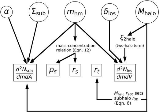
A graphical representation of the dark matter parameters in q_s: α, the logarithmic slope of the SHMF, Σ_sub, the overall scaling of the SHMF, m_hm, the WDM half-mode mass, δ_los, the overall factor for the line-of-sight halo mass function, and M_halo, the main deflector’s parent halo mass. ξ_2halo is implemented through equation (9) (see Section 3.3). These parameters are linked to the physical dark matter quantities they affect. From left to right: the SHMF |$\frac{\mathrm{ d}^2 N}{\mathrm{ d}m \mathrm{ d}A}$|⁠, the normalization ρ_s, scale radius r_s, and truncation radius r_t of individual haloes (see equation 5), and the line-of-sight halo mass function |$\frac{\mathrm{ d}^2 N}{\mathrm{ d}m \mathrm{ d}V}$|⁠. The priors for each of these parameters are summarized in Table 2, and discussed at length in Section 5.

5.7 The main deflector lens model

The galaxies that dominate the lensing cross-section are typically massive early-types with stellar velocity dispersions |$\sigma \gt 200 \ \rm {km} \ \rm {sec^{-1}}$| (Gavazzi et al. 2007; Auger et al. 2010; Lagattuta et al. 2010). The mass profiles of these systems are typically inferred to be isothermal, or close to isothermal (Treu et al. 2006, 2009; Auger et al. 2010; Shankar et al. 2017). These observations motivate a simple parametrization for the main deflector lens model, the singular isothermal ellipsoid plus external shear. We generalize this model to a power-law ellipsoid with a variable logarithmic slope γ_macro to account for uncertainties associated with the mass profile of the lensing galaxy, and the model-predicted flux ratios. We assume a flat prior on the power-law slope γ_macro between 1.95 and 2.2 for each deflector (Auger et al. 2010).

In addition to the logarithmic slope of the main deflector mass profile, we sample values for the external shear strength γ_ext. The prior for γ_ext is chosen on a lens-by-lens basis by first sampling the macromodel parameter space without subhaloes to determine a reasonable starting range for γ_ext. The width and centre of the prior is adjusted after adding substructure such that the posterior distribution of γ_ext obtained for each lens is contained well within the bounds of the prior. The specific priors used for each system are summarized in Table 2. Finally, we use a Gaussian prior for the mass centroid of each quad centred on the main deflector light with a variance of 0.05 arcsec, a typical modelling uncertainty for quadruple-image systems (Nierenberg et al. 2019; Shajib et al. 2019).

Several studies (Evans & Witt 2003; Hsueh et al. 2016, 2017, 2018; Gilman et al. 2017) explore the role of complicated main deflector morphologies on the model predicted flux ratios. As image magnifications are local probes of the gravitational potential, if there are fluctuations in the surface mass profile on scales comparable to the image separation these structures can affect the image magnifications. In particular, stellar discs, if they go unnoticed, can result in systematically inaccurate lens models. With deep Hubble Space Telescope (HST) images of the narrow-line quads in our sample, we can confirm that they do not contain discs, and indeed are representative of the massive elliptical galaxies with roughly isothermal mass profiles that typically act as strong lenses (Auger et al. 2010; Shankar et al. 2017). Gilman et al. (2017) and Hsueh et al. (2018) quantified the systematic uncertainties introduced by modelling early-type galaxy lenses as isothermal ellipsoids with fixed logarithmic slopes γ = 2. These works found that the resulting systematic uncertainties on image magnifications are typically less than |$10\, {\rm per\, cent}$|⁠. This degree of uncertainty is comparable to the variance in model-predicted image magnifications resulting from marginalizing over a power-law ellipsoid mass model with additional degrees of freedom implemented through a variable logarithmic slope γ (Nierenberg et al. 2019). Based on these considerations, we use a power-law ellipsoid with variable logarithmic slopes γ to model the main deflector mass profile.

Three quads in our sample do not have measured spectroscopic redshifts. For two of these, we use photometry from Shajib et al. (2019) to compute photometric redshifts probability distributions with the software eazy (Brammer, van Dokkum & Coppi 2008), and sample the deflector redshift from these distributions in the forward model. For the third system (WFI 2026), which does not have multiband photometry from Shajib et al. (2019), we assume a typical velocity dispersion for a massive elliptical galaxy, and derive a probability distribution for the lens redshift from measured quantities such as the source redshift and measured image separation. We give more details regarding this procedure in Appendix  B.

5.8 Satellite galaxies and nearby deflectors

We model satellite galaxies and other deflectors near the main lens as Singular Isothermal Spheres, and assume they lie at the lens redshift unless they have measured redshifts that place them elsewhere. We marginalize over the position and Einstein radius of these objects using Gaussian priors on the positions centred on the light centroid with a variance of 0.05 arcsec. We use a Gaussian prior on the Einstein radius which is estimated from lens model fitting, or in some cases by direct measurements on the central velocity dispersion (e.g. Wong et al. 2017; Rusu et al. 2019).

In the cases of HE0435 and WFI 2033, the nearby galaxy lies at a higher redshift than the main lens plane. The light from the galaxy is therefore subject to lensing by the main deflector, and its true physical location differs from its observed position. We estimate the true physical locations of these objects by sampling the macromodel parameter space using the image positions as constraints, and read out the physical position of background satellite given its observed (lensed) position. We then place the satellite at this derived physical location in the forward model sampling with uncertainties of 0.05 arcsec. This process significantly speeds up the lensing computations since it does not require the continuous re-evaluation of the physical satellite location given its observed position during each lens model computation.¹⁰ The boost in speed comes at the cost of decoupling the satellite galaxy position from the dark matter parameters q_s in the inference, but we expect the covariance between these quantities will be negligible because the satellite galaxies, even when their locations are corrected for foreground lensing effects, are relatively far from the images, introducing convergence at the main deflector light centroid of <0.1 in both cases.¹¹

In the case of HE0435, we estimate the angular location without foreground lensing of the satellite to be (−2.37, 2.08), while for WFI 2033 we obtain (−3.63, −0.08), for observed (lensed) locations of (−2.911, 2.339) and (−3.965, −0.022), respectively. These coordinates are with respect to the galaxy light centroid (see Table C1). The angular locations of the lensed background satellites are closer to the mass centroid of the main deflector, just as the physical location of the lensed background quasar is concentric with the mass centroid.

The lens-specific priors on satellite galaxies are summarized in Table 2.

5.9 Lens-specific modelling for RX J0911+0551 and WGD 2038–4008

For system RX J0911, we alter the modelling strategy slightly to increase computational efficiency by allowing the external shear strength γ_ext to vary freely while solving for macromodel parameters that fit the observed image positions. For the system WGD 2038, we widen the prior on the power-law slope of the macromodel as the posterior using the default range for γ_macro between 1.95 and 2.2 is biased towards higher values of γ_macro. For WGD 2038, the posterior peaks at γ_macro ∼ 2.25.

6 RESULTS

In this section, we present the results of our analysis. We begin in Section 6.1 by showing dark matter halo convergence maps for some of the top-ranked realizations drawn in the forward model. We then display the posterior distributions for a few individual lenses, showing the simultaneous inference of parameters describing the macro lens model and the dark matter hyper-parameters. In Section 6.2, we present the constraints on the abundance of substructure and dark matter warmth for the full sample of 11 quads.

6.1 Top-ranked realizations and posteriors for individual lenses

Minimizing the summary statistic in equation (4) selects realizations that resemble the observed data as closely as possible. This guarantees that the set of accepted dark matter hyper-parameters q_s yield an accurate approximation of the true posterior distribution for each individual lens with data d_n: p(q_s|d_n). For visualization purposes, and to reinforce the fact that the top-ranked realizations look like the data and satisfy S_lens ≈ 0 (equation 4), in Fig. 5 we display the dark matter halo effective multiplane convergence maps for some of the top-ranked realizations for a subset of quads in our sample. The effective multiplane convergence is defined as half the divergence of the full deflection field |$\boldsymbol{\alpha }$|

$$\begin{eqnarray*} \kappa _{\rm {effective}} \equiv \frac{1}{2} \ \nabla \cdot { \boldsymbol{\alpha }}. \end{eqnarray*}$$

(13)

This definition of the multiplane convergence accounts for the non-linear effects present in multiplane lensing, and satisfies the single-plane definition of convergence as second derivatives of a lensing potential in the absence of multiple lens planes.

Figure 5.

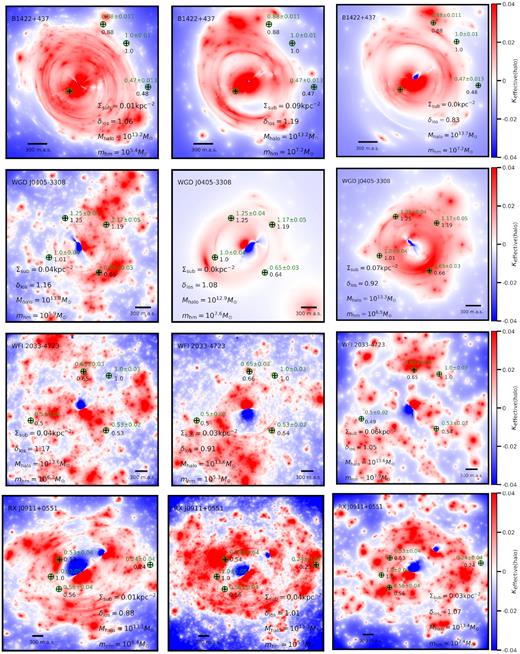
Dark matter halo effective multiplane convergence maps for some of the highest ranked realizations for the subset of quads B1422, WGD J0405, WFI 2033, and RX J0911, each of which has flux ratios inconsistent with smooth lens models. The definition of the effective multiplane convergence takes into account the non-linear effects present in multiplane lensing, and is defined with respect to the mean dark matter density in the Universe such that some regions are underdense (blue), while other regions (specifically, dark matter haloes) are overdense (red). The SHMF normalization, line-of-sight normalization, halo mass and half-mode mass are displayed for each realization. The green text/circles denote observed image positions and fluxes, while the black text/crosses denote the model positions and fluxes. The forward-model data sets fit the image positions and fluxes to within the measurement uncertainties.

To visualize individual realizations of dark matter structure, we define κ_{effective(halo)} ≡ κ_effective − κ_macro, where κ_macro is the convergence from the lens macromodel, including satellite galaxies and nearby deflectors. In the resulting convergence maps, haloes located behind the main lens plane appear sheared tangentially around the Einstein radius due to coupling to the large deflections produced by the macromodel.

In Fig. 5, we show κ_{effective(halo)} maps of randomly selected realizations of dark matter structure whose corresponding q_s parameters were accepted in the final posterior on the basis of their summary statistic S_lens. The specific realizations and the corresponding dark matter parameters q_s correspond to a diverse set of substructure populations, warm and cold, which yield similarly good fits to the observed flux ratios satisfying S_lens ∼ 0. Some models, however, predict flux ratios that match the observed flux ratios more frequently than others. In terms of the Approximate Bayesian Computing algorithm described in Section 2, the frequency with which one dark matter model relative to another predicts observables that resemble the data is a surrogate for the relative likelihood of the models. The probability of accepting a proposed q_s based on the summary statistic in equation (4) is therefore equal to the likelihood p(d_n|q_s) (equation 2), even though the form of this function is unknown and it is never directly evaluated.

The top-ranked realizations for B1422 shown in Fig. 5 each have a relatively massive dark matter halo, or several smaller ones, located near the top left merging triplet image with (normalized) flux 0.88. This is in agreement with the analysis by Nierenberg et al. (2014), who find that a blob of dark matter near this image brings the model-predicted flux ratios into agreement with a smooth lens model.

Although not obvious from examining Fig. 5, the underlying macromodels for each accepted realization are unique, with different external shears, power-law slopes, lens ellipticity, etc. We marginalize over different macromodel configurations by simultaneously sampling the macromodel parameters and the dark matter hyper-parameters in the forward model. To illustrate, in Figs 6, 7, and 8 we show the posterior distributions for several parameters in the lens macromodel, along with the dark matter hyper-parameters Σ_sub and m_hm for HE0435, WFI 2033, and RX J0911. The system HE0435 generally favours models with low SHMF normalizations (low Σ_sub), or a turnover in the mass function with higher Σ_sub. The system WFI 2033 is the opposite, with a posterior favouring CDM-like mass functions with many lens plane subhaloes. The system RX J0911 lies somewhere in between, with a peak in the posterior distribution of m_hm near 10⁷ M_⊙.

Figure 6.

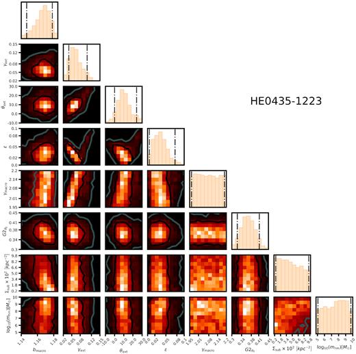
Joint posterior distribution for a subset of M and q_s parameters for the system HE0435. We display the normalization of the main deflector lens model b_macro, the external shear strength and position angle γ_ext and θ_ext, the deflector ellipticity ϵ, the power-law slope of the main deflector mass profile γ_macro, the Einstein radius of the satellite galaxy |$G2_{\theta _E}$|⁠, the normalization of the SHMF Σ_sub, and the half-mode mass m_hm. We simultaneously sample the distributions of these parameters to account for covariance between the macromodel and the dark matter hyper-parameters q_s. The vertical lines denote |$95\, {\rm per\, cent}$| confidence intervals.

Figure 7.

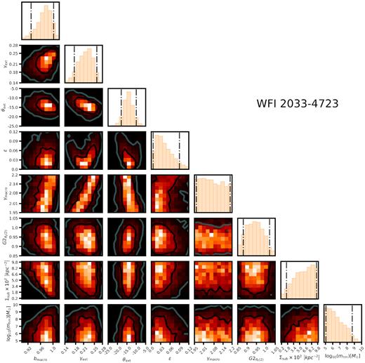
Joint posterior distribution for a subset of M and q_s parameters for the system WFI 2033. The parameters are the same as in Fig. 6. In addition to the main deflector we model two additional nearby galaxies, with Einstein radii |$G2_{\theta _E(1)}$| and |$G2_{\theta _E(2)}$|⁠. We show the distributions of the Einstein radius for the larger nearby galaxy (⁠|$G2_{\theta _E(2)}$|⁠), whose position we correct for foreground lensing effects (see Section 5.8).

Figure 8.

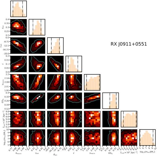
Joint posterior distribution for a subset of M and q_s parameters for the system RX J0911. The parameters are the same as in Fig. 6.

For each of these systems, in particular WFI 2033, there is a visibly obvious covariance between the overall normalization of the main deflector mass profile b_macro,¹² and the parameters Σ_sub and m_hm. This covariance is readily understood: To reproduce the observed image positions, the macromodel responds to the addition of mass in the form of subhaloes in main lens plane by decreasing the overall normalization of the main deflector mass profile, and hence these quantities are anticorrelated. Similarly, WDM models correspond to macromodels with larger b_macro because WDM realizations contain fewer subhaloes. Interestingly, there is some structure in the posterior distribution for the lens ellipticity ϵ in WFI 2033, and both m_hm and Σ_sub.

By simultaneously sampling the lens macromodel and dark matter hyper-parameters, we obtain posterior distributions that account for covariance between M and q_s. We do not use lens model priors from more sophisticated lens modelling efforts (e.g. Wong et al. 2017; Shajib et al. 2019) because these analyses did not include substructure in the lens models and therefore do not account for covariances between the macromodel parameters and the dark matter parameters of interest. For the same reason, we do not decouple the lens macromodel parameters from the dark matter hyper-parameters by first sampling the macromodel parameter space that fits the image positions, and using these distributions as priors in the forward modelling.

6.2 Constraints on the free-streaming length of dark matter

For each quad, we obtain a joint likelihood between the macromodel parameters M and the dark matter-hyper parameters q_s. We marginalize over the parameters in this 20+dimensional space to obtain the four-dimensional space of q_s parameters that includes logarithmic slope of the SHMF α, the scaling of the line-of-sight halo mass function δ_los, the overall scaling of the SHMF Σ_sub, and the half-mode mass m_hm. We reiterate that these four parameters describe universal properties of dark matter and should therefore be common to all the lenses, while the parameters M and the halo mass M_halo are lens-specific. After marginalizing, we compute the product of the resulting likelihoods and obtain the desired posterior distribution in equation (1), which we display in Fig. 9.

Figure 9.

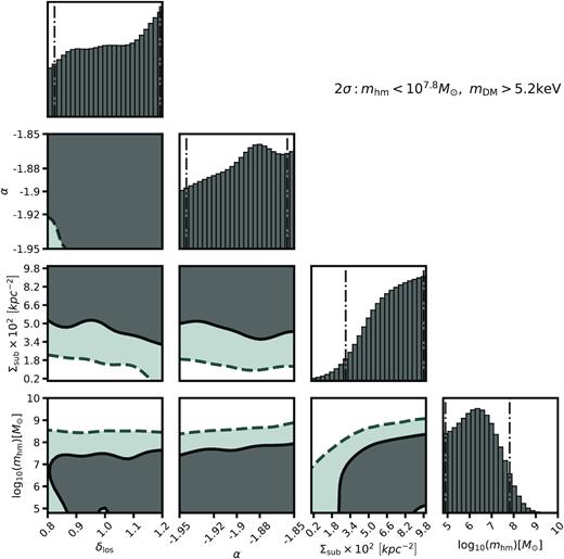
Marginal and joint posterior distributions for the dark matter hyper-parameters δ_los, α, Σ_sub, and m_hm, which represent the overall scaling of the line-of-sight halo mass function, the logarithmic slope of the SHMF, the global normalization of the SHMF that accounts for evolution with halo mass and redshift (see equation 7), and the half-mode mass m_hm relevant to WDM models. The contours show |$68\, {\rm per\, cent}$| and |$95\, {\rm per\, cent}$| confidence intervals, while the dot–dashed lines on the marginal distributions show the |$95\, {\rm per\, cent}$| confidence intervals.

The marginalized constraints on m_hm rule out m_hm > 10^7.8 M_⊙ at 2σ, corresponding to thermal relic particle mass of |$\lt 5.2\,\rm {keV}$|⁠. It is apparent from Fig. 9 that m_hm and Σ_sub are correlated, since haloes added by increasing the normalization can be subsequently removed by increasing m_hm such that the total amount of lensing substructure remains relatively constant. As a result, the marginalized distribution for the normalization Σ_sub appears unconstrained from above, as the normalization can be significantly higher in WDM scenarios. With only eight quads we cannot simultaneously measure m_hm and Σ_sub, although our previous forecasts indicate this is possible with more lenses (Gilman et al. 2018).

The constraints on dark matter warmth in terms of confidence intervals depend on the range of allowed values specified by the prior on Σ_sub. Similarly, the confidence interval on m_hm depends on the lower bound of this parameter that is set by the prior on m_hm. As discussed in Section 5.5, we have chosen the prior on m_hm to encompass the region of parameter space where the data can constrain m_hm, keeping in mind that the WDM mass–concentration relation affects the central densities of subhaloes 60 times above m_hm (equation 12), and the upper bound of |$\Sigma _{\rm {sub}} = 0.1 \,\rm {kpc^{-2}}$| is a conservative choice as most N-body simulations and the galacticus runs predict values below |$0.05 \,\rm {kpc^{-2}}$|⁠. In light of these complications, we also quote likelihood ratios which do not depend on the choice of prior. Relative to the peak of the m_hm posterior, we obtain likelihood ratios for WDM with m_hm = 10^8.2 M_⊙ (m_hm = 10^8.6 M_⊙) of 7:1 (30:1).¹³

The posterior for δ_los indicates the data favour more line-of-sight structure, but the preference is not statistically significant. The parameters δ_los and Σ_sub are anticorrelated, as one would expect as one can, to a certain degree, remove lens plane subhaloes and replace them with line-of-sight haloes while keeping the total amount of flux perturbation constant. This is not a perfect degeneracy, however, since lensing efficiency and the relative number of subhaloes and line-of-sight haloes changes with redshift. Thus, a larger sample of quads at different redshifts could break the covariance between Σ_sub and δ_los.

6.3 Constraints on the subhalo mass function assuming CDM

We perform a suite of CDM simulations using the same priors listed in Table 2, minus the WDM parameter m_hm, with the aim of inferring Σ_sub. We marginalize over δ_los, and over a theoretical-motivated prior on α (between −1.95 and −1.85) based on predictions from N-body simulations (Springel et al. 2008; Fiacconi et al. 2016).

The inference on Σ_sub is shown in Fig. 10. We infer |$\Sigma _{\rm {sub}} = 0.055 \,\rm {kpc^{-2}}$|⁠, with a 1σ confidence interval |$0.029 \lt \Sigma _{\rm {sub}} \lt 0.083 \ \rm {kpc^{-2}}$|⁠. At the 2σ level we obtain |$\Sigma _{\rm {sub}} \gt 0.008 \ \rm {kpc^{-2}}$|⁠. We do not quote an upper 2σ bound on Σ_sub as it is prior dominated. To put these numbers in physical units, the mean value of Σ_sub corresponds to a mean projected mass in substructure for the lenses in our sample between 10⁶ and 10⁹ M_⊙ of |$4.0 \times 10^{7}\, {{\rm M}_{\odot }}\ \rm {kpc^{-2}}$|⁠, and the 1σ confidence interval corresponds to |$2.0{-}6.1 \times 10^{7}\, {{\rm M}_{\odot }}\,\rm {kpc^{-2}}$|⁠. At 2σ, the projected mass constraint is |$\Sigma _{\rm {sub}} \gt 0.6 \times 10^{7} {{\rm M}_{\odot }}\rm {kpc^{-2}}$|⁠. To convert into the average projected mass, we have computed the average of the projected masses for each of the eight lenses in our sample, using the scaling of the halo mass function with redshift in equation (8) while assuming a halo mass of 10¹³ M_⊙.

Figure 10.

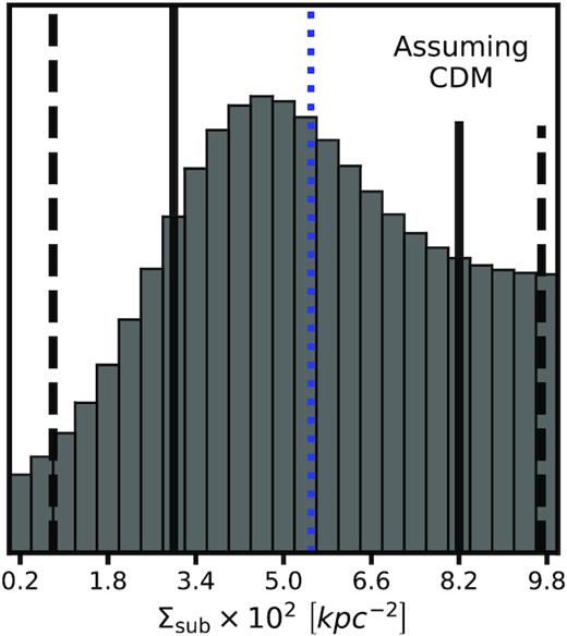
Inference on the global normalization of the SHMF Σ_sub assuming CDM, marginalized over the logarithmic slope α and uncertainty in the overall amplitude of the line-of-sight halo mass function δ_los. The blue dashed lines shows the mean of the marginal distribution, while the black solid (dashed) lines represent |$68\, {\rm per\, cent}$| and |$95 \, {\rm per\, cent}$| confidence intervals. The contours in the joint distribution also represent |$68\, {\rm per\, cent}$| and |$95 \, {\rm per\, cent}$| confidence intervals.

7 DISCUSSION AND CONCLUSIONS

In this section, we review the main results of this work and discuss the implications for cold and warm dark matter. In Section 7.1, we summarize our main results, and in Section 7.2, we compare our results with those obtained in previous works. In Section 7.3, we discuss the sources of systematic uncertainty in our analysis, and we conclude in Section 7.4 by discussing the implications of our result for cold and warm dark matter.

7.1 Summary of the analysis and main results

We have carried out a measurement of the free-streaming length of dark matter and the SHMF using a sample of eight quadruply imaged quasars. The methodology we use to constrain the dark matter parameters of interest has been tested and verified with simulated data (Gilman et al. 2019). Lenses that show evidence for morphological complexity in the form of stellar discs are excluded from our analysis. We model haloes both in the main deflector and along the line of sight, including correlated structure around the main deflector through the two-halo term, and account for evolution of the projected SHMF with redshift and halo mass using a suite of simulations using the semi-analytic modelling code galacticus. We compute image flux ratios by ray-tracing to finite-size background sources, which correctly accounts for the sensitivity of image flux ratios to perturbing haloes. We also marginalize over the macromodel parameters for each system, including the power-law slope of the main deflector, and simultaneously constrain the lens macromodel and dark matter hyper-parameters to account for covariance between these quantities. In addition to the turnover in the halo mass function, we model WDM free-streaming effects on the mass–concentration relation, accounting for the effect of reduced central densities of WDM haloes on lensing observables.

The main results of this analysis are summarized as follows:

• We constrain the half-mode mass m_hm (thermal relic dark matter particle mass) to m_hm < 10^7.8 M_⊙ (⁠|$m_{\rm {DM}} \gt 5.2 \,\rm {keV}$|⁠) at 2σ. Since the confidence intervals depend on the prior used for both m_hm and Σ_sub, we also quote likelihood ratios relative to the peak of the posterior distribution for m_hm: we disfavour m_hm = 10^8.2 M_⊙ (⁠|$m_{\rm {DM}} = 4 \,\rm {keV}$|⁠) with a likelihood ratio of 7:1, and with m_hm = 10^8.6 M_⊙ (⁠|$m_{\rm {DM}} = 3.0 \,\rm {keV}$|⁠) the relative likelihood is 30:1. These bounds are marginalized over the amplitude of the SHMF, the amplitude of the line-of-sight halo mass function, the power-law slope of the SHMF, the parent halo mass, the background source size, and the parameters describing the main deflector mass profile.

• Assuming CDM, we infer a value of the global amplitude of the SHMF|$\Sigma _{\rm {sub}} = 0.055_{-0.027}^{0.032} \rm {kpc^{-2}}$| at 1σ, and |$\Sigma _{\rm {sub}} \gt 0.008 \rm {kpc^{-2}}$| at 2σ. In our lens sample, these values correspond to an average projected mass density in substructure between 10⁶ and 10⁹ M_⊙ of |$4.0_{-2.0}^{+2.1} \times 10^{7} {{\rm M}_{\odot }}\rm {kpc^{-2}}$| and a lower bound of |$0.6 \times 10^{7}\, {{\rm M}_{\odot }}\,\rm {kpc^{-2}}$|⁠, respectively. At fixed redshifts, for a 10¹³ M_⊙ halo at z = 0.2 (z = 0.6) the 1σ constraint corresponds to a projected mass in substructure of |$1.9_{-0.9}^{+0.9} \times 10^7\, {{\rm M}_{\odot }}\,\rm {kpc^{-2}}$| (⁠|$4.1_{-2.0}^{+2.0} \times 10^7 \,{{\rm M}_{\odot }}\,\rm {kpc^{-2}}$|⁠) in the subhalo mass range 10⁶–10⁹ M_⊙. The 2σ constraint corresponds to a projected mass in substructure of greater than |$0.3 \times 10^7 \,{{\rm M}_{\odot }}\,\rm {kpc^{-2}}$| (⁠|$0.6 \times 10^7 \,{{\rm M}_{\odot }}\,\rm {kpc^{-2}}$|⁠) in the same mass range.

7.2 Discussion and comparison with previous work

7.2.1 Constraints on dark matter warmth and the amplitude of the CDM subhalo mass function

The first comprehensive analysis of multiply-imaged quasars was carried out by DK2, who inferred a projected mass fraction in substructure |${\bar{f}_{\rm {sub}}}$|¹⁴ in the range |$0.006 \lt {\bar{f}_{\rm {sub}}}\lt 0.07$| at 2σ modelling only lens-plane substructure, and assuming CDM. Recently, H19 improved on the analysis of DK2 by including the effects of line-of-sight haloes, measuring |$0.006 \lt {\bar{f}_{\rm {sub}}}\lt 0.018$| at 1σ with a mean of 0.011 assuming CDM, and also constrained the free-streaming length of dark matter to m_hm < 10^8.4 (⁠|$m_{\rm {DM}} \gt 3.8 \,\rm {keV}$|⁠).

The 2σ bound from H19 of m_hm < 10^8.4 M_⊙ is weaker than the constraint from this work m_hm < 10^7.8 M_⊙. One possible reason for this difference is that unlike previous work (Birrer et al. 2017b; Gilman et al. 2018, 2019) H19 did not model the suppression of the mass–concentration relation in WDM scenarios, which suppresses the lensing signal more than one order of magnitude above the position of the turnover in the mass function. This is of particular relevance for flux ratio studies because the effect of a perturbing dark matter halo depends on its central density profile. Free-streaming effects on the mass–concentration relation therefore increase the relative differences between CDM and WDM on the scales relevant for substructure lensing, which leads to greater constraining power over WDM models. Finally, we note that in a future analysis modelling the tidal evolution of substructures from the time of infall to the time of lensing may introduce additional constraining power over WDM models by coupling the structural parameters of subhaloes at the time of lensing to their structural properties, such as concentration, at the time of infall.

To facilitate direct comparison between this analysis and that of DK2 and H19 regarding the constraints on the SHMF assuming CDM, we convert our Σ_sub values into estimates of |${\bar{f}_{\rm {sub}}}$| by computing the projected mass density Σ, and then using the fact that |$\frac{\Sigma }{\Sigma _{\rm {crit}}} = 0.5$| near the Einstein radius, where Σ_crit is the critical surface mass density for lensing. In these conversions, we also assume a halo mass of 10¹³ M_⊙, and take care to compute |${\bar{f}_{\rm {sub}}}$| using the same mass range 10⁶–10⁹ M_⊙ used by H19. Our 2σ bounds on Σ_sub correspond to an average mass fraction in substructure |${\bar{f}_{\rm {sub}}}\gt 0.005$| with a mean of |${\bar{f}_{\rm {sub}}}= 0.035$|⁠. At 1σ |$0.018 \lt {\bar{f}_{\rm {sub}}}\lt 0.056$|⁠. This result is statistically consistent with the constraints from H19, and also with those of DK2.

There are several key differences between our analysis and those of H19 and DK2 that pull in opposite directions in terms of constraining power over dark matter models. As mentioned previously we model free-streaming effects on the mass–concentration relation, and include the contribution from the two-halo term to account for correlated structure near the main deflector. These pieces of additional physics add information and increase our constraining power over WDM models. On the other hand, accounting for finite-size background sources decreases the expected magnification signal caused by dark matter haloes and subhaloes, and we expect to infer a higher normalization of the SHMF in our analysis as more substructure is needed to produce the same degree of flux perturbation. Explicitly, by ray-tracing to finite-size background sources we find that the peak of the magnification cross-section for a 5 × 10⁷ M_⊙ halo is reduced by a factor of two for a |$15 \,\rm {pc}$| background source relative to a |$5 \,\rm {pc}$| background source, and by a factor of three for a |$40 \,\rm {pc}$| source. The simplifying assumption of point-sources for the background quasar invoked by H19 and DK2 introduces signal from low-mass haloes whose effects would otherwise be washed out by an extended source.

The tidal truncation of lens plane subhaloes that we model may also reduce the overall impact of subhaloes on lensing observables. We also marginalize over the power-law slope of the main deflector and simultaneously sample the macromodel parameters and the dark matter hyper-parameters. These processes introduce additional covariances in the posterior distributions, and should lead to weaker constraints on Σ_sub and m_hm.

Other lensing studies, primarily those using the technique of gravitational imaging, have also sought to measure the SHMF. Vegetti et al. (2014) inferred |${\bar{f}_{\rm {sub}}}= 0.0064_{-0.0042}^{0.0080}$| at 1σ in the mass range 4 × 10⁶–4 × 10⁹ M_⊙ assuming a prior on the slope of the SHMF centred on α = −1.9, while Hezaveh et al. (2016b) constrained the normalization of SHMF assuming α = −1.9, inferring |$\bar{f}_{\rm {fsub}}$| values comparable to the median |$\bar{f}_{\rm {sub}} = 0.02$| result from DK2 (and our constraint), but with larger uncertainties.

To compare with the analysis of Vegetti et al. (2014), we assume a halo mass of 10¹³ M_⊙ at a lens redshift z_d = 0.25 and a source at z_src = 0.7, characteristic values for the lens sample analysed by Vegetti et al. (2014). Using these values with our expression for the SHMF in equation (7), we obtain |${{f}_{\rm {sub}}}= 0.014_{-0.007}^{+0.008}$| between 4 × 10⁶ and 6 × 10⁹ M_⊙ at 1σ, in the same mass range used by Vegetti et al. (2014). This result is consistent with that of Vegetti et al. (2014).¹⁵ We quote constraints on f_sub to make comparisons with previous work, but we caution that the conclusions derived from inferences of f_sub should be interpreted with care. The physical meaning of this parameter depends on specific assumptions regarding the subhalo mass range and the contribution from dark substructure to the convergence near the Einstein radius, which may change with halo mass and redshift.

Comparing our results with semi-analytic simulations of massive 10¹³ M_⊙ hosts, our results in terms of the projected mass in substructure is consistent with the galacticus simulations used to calibrate the evolution of the SHMF with halo mass and redshift. We stress that our model was not tuned to match the normalization predicted by galacticus, it only made use of the trends of projected substructure mass density with host halo mass and redshift.

Our results are also consistent with N-body simulations of 10¹³ M_⊙ haloes by Fiacconi et al. (2016), who predict projected substructure mass densities of |$2.0{-}2.8 \times 10^{7} \,{{\rm M}_{\odot }}\,\rm {kpc^{-2}}$| after accounting for baryonic contraction of the halo. We infer roughly triple the predicted mass in substructure than the amount predicted by Xu et al. (2015), who simulated 10¹³ M_⊙ haloes by rescaling Milky Way size and cluster size hosts to halo masses of ∼10¹³ M_⊙. Finally, we note that our results arrive on the heels of several works that examine numerical features of N-body simulations that may result in the artificial fragmentation of subhaloes (van den Bosch et al. 2018; Errani & Peñarrubia 2019). Taken at face value, these results suggest that N-body simulations may underpredict substructure abundance in dark matter haloes.

We may also compare our constraints with the projections from Gilman et al. (2019). With a sample of 10 quads, they projected a 2σ bound on m_hm with |$\Sigma _{\rm {sub}} = 0.022\, \rm {kpc^{-2}}$| of 10^7.7 M_⊙ with |$2\, {\rm per\, cent}$| uncertainties in image fluxes, and 10^8.6 M_⊙ with |$6 \, {\rm per\, cent}$| uncertainties. Our constraint of m_hm < 10^7.8 M_⊙ is broadly consistent with these predictions,¹⁶ given the higher mean Σ_sub value of |$0.055 \,\rm {kpc^{-2}}$| we infer in this analysis, and the flux uncertainties in the lens sample which are |${\sim}6 \, {\rm per\, cent}$| on average.

The overall scaling of the line-of-sight halo mass function δ_los is unconstrained with our sample size and choice of prior. This is likely because the prior on δ_los spans a relatively limited range of |${\pm}20\, {\rm per\, cent}$| around the Sheth–Tormen mass function prediction, and with the current sample size of only eight quads we cannot constrain departures from the Sheth–Tormen prediction at the level of |$10{-}20\, {\rm per\, cent}$|⁠.

7.3 Sources of systematic uncertainties

7.3.1 The lens macromodels

Several works (Gilman et al. 2017; Hsueh et al. 2018) have investigated the ability of smooth isothermal mass models plus external shear to fit the smooth mass component of galaxy scale strong lenses. These works reach similar conclusions, determining that isothermal models predict image flux ratios to better than |$10 \, {\rm per\, cent}$| unless a stellar disc is present, in which case explicit modelling of the disc is required (e.g. Hsueh et al. 2017, 2018). Each of these analysis restricted the smooth lens models to exactly isothermal mass density profiles.

The deflectors in our sample show no evidence for morphological complexity that would require explicit modelling beyond a power-law ellipsoid model. Specifically, we exclude all lens systems with known stellar discs to avoid any bias they may introduce. To account for remaining uncertainties associated with the lens macromodel, we highlight two features of our lens modelling implemented in an effort to mitigate this source of systematic uncertainty. First, we note that flux ratios are highly localized probes of the surface mass density in the immediate vicinity of the lensed images, and therefore the main requirement for this work is to accurately predict the mass profile in these four small isolated regions. By relaxing the strictly isothermal mass profile assumption and marginalizing over the logarithmic slope of the main deflector mass profile, we allow for the local mass profile in the vicinity of the lensed images to vary. The additional degree of freedom added in the lens macromodel increases our uncertainties, but accounts for deviations from power-law ellipsoids limited to exact ρ(r) ∝ r⁻² mass profiles.

Second, we note that smooth power-law models predict a distribution of flux ratios, rather than single values (for example, see figs A1–A8 in Nierenberg et al. 2019). Following common practice, Gilman et al. (2017) and Hsueh et al. (2018) identified flux ratio ‘anomalies’ with respect to a single smooth model fit to lensed images, a procedure that does not account for the distribution of flux ratios predicted by smooth lens models that is marginalized over in the full forward-modelling analysis we perform. In this work, we also take care to explore the macromodel parameter space and the dark matter hyper-parameter space simultaneously, which accounts for additional covariances that contribute to the model-predicted flux uncertainties.

7.3.2 Modelling of the dark matter content

We assume specific functional forms for the halo and SHMFs (equations 7 and 9), and the mass–concentration–redshift relation (equation 12). We acknowledge that there are other parametrizations in the literature for both of these quantities (e.g. Schneider et al. 2012; Benson et al. 2013), but in this work we implement only one parametrization of WDM effects on the mass function (equation 11) and halo concentrations (equation 12), which corresponds to one specific WDM model. We note that additional physics, such as the velocity dispersion of dark matter particles in the early Universe, can alter the shape of the mass function, but with the current sample size of lenses it is unlikely we have enough information to constrain these additional features if they were included in the model.

It is possible that free-streaming effects on the halo mass function near the half-mode mass scale may become more pronounced at high redshifts. This could affect both the location and shape of the turnover in the mass function. However, in the absence of a specific prediction for the evolution of the turnover with redshift, we apply the parametrization in equation (11) through the relevant redshift range z = 0–3.5. We note that since the lensing efficiency of haloes decreases approaching source redshift, systematic errors from possible redshift evolution of the WDM turnover will be correspondingly down-weighted. We note that the mass–concentration–redshift relation for WDM calibrated by Bose et al. (2016) that we implement does evolve with redshift, as does the CDM mass–concentration relation from Diemer & Joyce (2019).

7.4 Implications for WDM models

Galaxy–galaxy strong lensing provides a useful compliment to the strongest existing probe of the free-streaming length of dark matter from the Lyman-α forest (Viel et al. 2013; Iršič et al. 2017). Our 2σ bound on the thermal relic mass of |$m_{\rm {DM}} \gt 5.2 \,\rm {keV}$| surpasses than the 3.3 keV constraint from Viel et al. (2013) and matches the |$5.3 \,\rm {keV}$| constraint from Iršič et al. (2017), who invoked additional assumptions regarding the relevant thermodynamics. The key point of this comparison, however, is not so much which method achieves the most precision, but the fact that both methods provide stringent limits and that they are completely independent of each other in observational data and astrophysical assumptions. Independently and in combination, the results from lensing and the Lyman-α forest support the following statement: the halo mass function extends down in a scale-free manner to mass scales of ∼10⁸ M_⊙, where haloes are mostly, if not completely, dark. There appears to be little room left for a viable WDM solution to the small-scale issues of CDM.

ACKNOWLEDGEMENTS

We thank the anonymous referee for a careful reading of the paper and thoughtful comments. We are also grateful to Alex Kusenko and Annika Peter for useful discussions throughout the course of this project, and thank David Gilman for useful comments on an early draft version of this work.

DG, TT, and SB acknowledge support by the US National Science Foundation through grant AST-1714953. DG, TT, SB, and AN acknowledge support from HST-GO-15177. AJB and XD acknowledge support from NASA ATP grant 17-ATP17-0120. Support for Program number GO-15177 was provided by NASA through a grant from the Space Telescope Science Institute, which is operated by the Association of Universities for Research in Astronomy, Incorporated, under NASA contract NAS5-26555. TT and AN acknowledge support from HST-GO-13732. AN acknowledges support from the NASA Postdoctoral Program Fellowship, the UC Irvine Chancellor’s Fellowship, and the Center for Cosmology and Astroparticle Physics Fellowship.

This work used computational and storage services associated with the Hoffman2 Shared Cluster provided by the UCLA Institute for Digital Research and Education’s Research Technology Group. This work also used computational and storage services associated with the Aurora and Halo super computers. These resources were provided by funding from the JPL Office of the Chief Information Officer. In addition, calculations were performed on the memex compute cluster, a resource provided by the Carnegie Institution for Science.

Part of this work is based on observations made with the NASA/ESA Hubble Space Telescope, obtained at the Space Telescope Science Institute, which is operated by the Association of Universities for Research in Astronomy, Inc., under NASA contract NAS 5-26555. These observations are associated with programs |$\#13732$| and |$\#15177$|⁠. Support for programs |$\#13732$| and |$\#15177$| was provided by NASA through a grant from the Space Telescope Science Institute, which is operated by the Association of Universities for Research in Astronomy, Inc., under NASA contract NAS5-26555.

Footnotes

1

https://github.com/sibirrer/lenstronomy

2

The full set of macromodel parameters for a power-law ellipsoid are the overall normalization b_macro, the mass centroid g_x and g_y, the ellipticity and ellipticity position angle ϵ and θ_ϵ, the external shear and shear angle γ_ext and θ_ext, and the power-law slope γ_macro. Nearby galaxies are modelled as Singular Isothermal Spheres.

3

The four image positions provide 4 × 2 = 8 constraints, and the macromodel parameters that are allowed to vary freely, plus the source position, give eight degrees of freedom.

4

Before taking the product, we use a Gaussian kernel density estimator (KDE) with a first-order boundary correction (e.g. Lewis 2015) to obtain a continuous approximation of the likelihood for each lens. We compute the bandwidth according to Scott’s factor (Scott 1992), but caution that care should be taken with the choice of bandwidth to avoid oversmoothing or undersmoothing the likelihood.

5

Code version 7175:2bd6b8d84a39

6

The entire simulation suite using galacticus completed in 1000 CPU hours.

7

In appendix A of Gilman et al. (2019), we describe how this effect is implemented and show that this term contributes a |${\sim}4\, {\rm per\, cent}$| increase in the frequency of flux ratio perturbations induced by objects outside the virial radius of the main deflector.

8

We define r_vir with respect to the matter density contrast 200ρ_crit.

9

galacticus is capable of including the tidal stripping effects from a central galaxy, but we did not include them to minimize computation costs.

10

The physical location of the nearby galaxy needs to be continuously re-evaluated because it’s observed location depends on the foreground lensing effects from the macromodel, and the parameters describing the macromodel are continuously changing while finding a solution to the lens equation (equation 3).

11

The default convention in lenstronomy is to place deflectors at their observed angular locations in the Universe, but it is now possible (in code versions 0.8.0 +) to specify which objects should be treated using the observed (lensed) position instead. We note that the default convention in lensmodel (Keeton, Kochanek & Seljak 1997) is to place objects at their observed (lensed) locations during multiplane ray-tracing.

12

b_macro has units of convergence, or projected mass density divided by the critical surface mass density for lensing.

13

We remind the reader that the relative heights of the peaks in the posterior somewhat depend on the binning method, or in this case the bandwidth estimator of the KDE. In this work, we have applied a KDE with a first-order boundary correction and a bandwidth selected according to Scott’s factor (Scott 1992).

14

Throughout this section, we will use |${\bar{f}_{\rm {sub}}}$| to refer to the average mass fraction in substructure inferred from a sample of multiple lenses in haloes of different masses at different redshifts, and f_sub to refer to the mass fraction in substructure implied by a certain Σ_sub value at a specific redshift and halo mass.

15

Although Vegetti et al. (2014) did not model line-of-sight haloes, the low lens/source redshifts of their sample lessen the impact of line-of-sight haloes on the inferred subhalo mass fraction such that we may compare our results, which include line-of-sight haloes, with theirs.

16

The conversion between the half-mode mass and the mass of the corresponding thermal relic dark matter particle used by Gilman et al. (2019) is off by a factor of h = 0.7, but the comparison between the half-mode masses is robust.

APPENDIX A: CONVERGENCE OF THE POSTERIOR DISTRIBUTIONS

The approximation of the true posterior obtained in Approximate Bayesian Computing (ABC) algorithms converges to the true posterior distribution as the acceptance criterion becomes increasingly more stringent. In our framework, changing the acceptance criterion is equivalent to reducing the number of forward model samples while keeping the number of total accepted realizations fixed. We exploit this property to test for convergence of the posteriors.

In Figures A1 and A2, we compare posteriors constructed from the full set of forward model samples with others derived from a depleted set of forward model samples, where we have discarded one-third of the realizations and accepted the same rejection criterion (accept the realizations corresponding to the 800 lowest values of S_lens) to those that remain. The mass of the posterior distributions remains relatively unchanged, and the 1σ and 2σ contours are nearly identical. We conclude we have generated enough realizations of dark matter structure to reliably construct posterior distributions using the ABC rejection algorithm described in Section 2.

Figure A1.

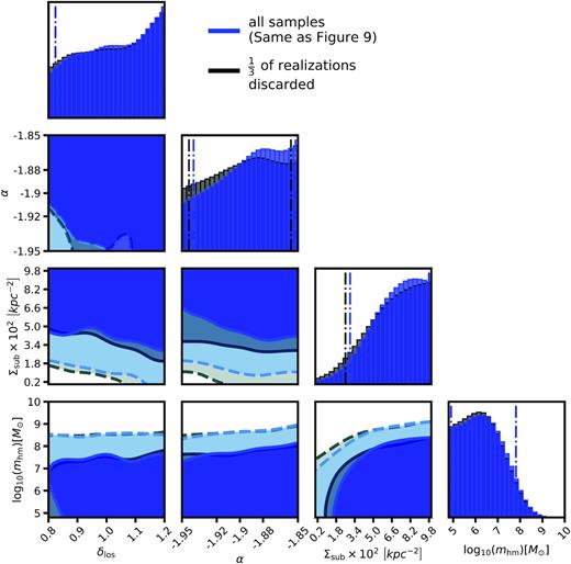
A convergence test of the posterior distributions. By discarding one-third of the forward model samples and applying the same rejection criterion to those that remain, we verify the inference obtained through the ABC rejection algorithm is robust.

Figure A2.

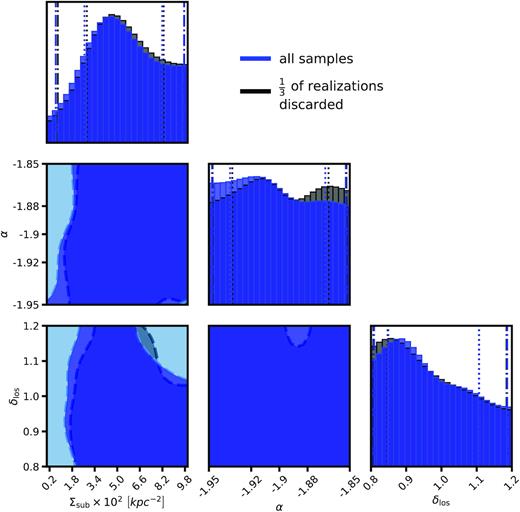
A convergence test of the posterior distributions assuming CDM. Like Fig. A1, one-third of the samples are discarded and the same number of realizations are accepted into the posterior.

APPENDIX B: OBTAINING DEFLECTOR REDSHIFTS

The quads PS J1606 and WGD J0405 do not have measured spectroscopic redshifts, so we use photometry from Shajib et al. (2019) to obtain photometric redshift estimates. The photometry from Shajib et al. (2019) comes in three bands: F160W, F814W, and F475X with magnitude uncertainties of 0.1–0.3 dex. We use the software package eazy (Brammer et al. 2008), and restrict the templates to only consider the SEDs for early-type galaxies, which are |$90\, \mathrm{ per}\, \mathrm{ cent}$| of galaxies acting as strong lenses. We verify this procedure is accurate by applying it to other deflectors in sample analysed by Shajib et al. (2019) that have measured spectroscopic redshifts, and then proceed to derive PDFs for deflector redshifts in the systems PS J1606 and WGD J0405.

The results are shown in Fig. B1. The top row shows four quads from the sample analysed in Shajib et al. (2019) with measured spectroscopic redshifts, and the bottom row shows the PDF’s output by eazy for the systems PS J1606 and WGD J0405.

Figure B1.

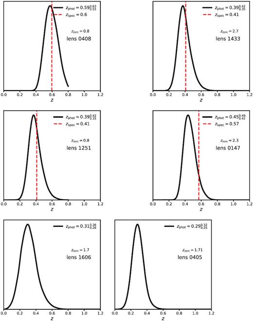
PDFs for main deflector redshifts computed with the software eazy and photometry from Shajib et al. (2019), restricting the photometry templates to those of early-type galaxies. The top rows show four applications of this procedure to quads with measured spectroscopic redshifts (red dotted lines). The bottom row shows the results of this procedure, using the same photometry and template assumptions, applied to the quads PS J1606 and WGD J0405, which do not have spectroscopic redshift measurements.

The system WFI 2026 does not have a photometric redshift, and the photometry available in the literature comes in only one or two bands with larger uncertainties. For this system, we use the equation for isothermal mass profiles relating the Einstein radius R_Ein, source redshift z_s, lens redshift z_d, velocity dispersion σ, and speed of light c

$$\begin{eqnarray*} R_{\rm {Ein}} = 4 \pi \left(\frac{\sigma }{c}\right)^2 \frac{D_{\rm {ds}}(z_\mathrm{ d}, z_\mathrm{ s})}{D_{\rm {s}}(z_\mathrm{ s})} , \end{eqnarray*}$$

(B1)

where D_ds and D_s are angular diameter distances between the lens and the source, and the observer and the source, respectively.

We sample a Gaussian distribution of velocity dispersions typical of early-type galaxies |$240 \pm 30 \rm {km} \rm {s^{-1}}$|⁠, evaluate the right-hand side of equation (B1), and numerically solve for the lens redshift that yields the resulting angular diameter distance. The resulting PDF shown in the bottom right panel of Fig. B2 peaks around z_d = 1, for the measured values R_Ein = 0.67 arcsec, z_s = 2.2. We have experimented with placing WFI 2026 at various specific redshifts, but find the posteriors for Σ_sub, δ_los, α, and m_hm are unchanged within the uncertainties.

Figure B2.

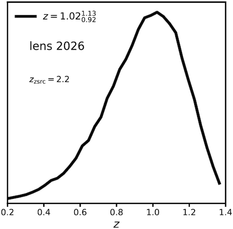
The PDF for the deflector redshift of WFI 2026 obtained by assuming a velocity dispersion of |$240 \pm 30 \ \rm {km} \ \rm {s^{-1}}$| and a roughly isothermal mass profile.

APPENDIX C: DATA

We summarize the data used in this analysis, and the references for the astrometry, fluxes or flux ratios, and the corresponding uncertainties, and satellite galaxies or nearby nearby deflectors in Table C1.

Table C1.

The data used in this analysis. Letters A–D correspond to the lensed images, while G is the galaxy light centroid. The priors sampled for the satellite galaxies or nearby deflectors are quoted in Table 2. Discovery papers are marked with a †.

Lens	Image	dRA	dDec.	NL flux
WGD J0405–3308	A	1.066 ± 0.003	0.323 ± 0.003	1.00 ± 0.04
Nierenberg et al. (2019)	B	0 ± 0.003	0 ± 0.003	0.65 ± 0.04
†Anguita et al. (2018)	C	0.721 ± 0.003	1.159 ± 0.003	1.25 ± 0.03
	D	−0.157 ± 0.003	1.021 ± 0.003	1.17 ± 0.04
	G	0.358 ± 0.05	0.567 ± 0.05	–
HE0435–1223	A	2.424 ± 0.008	0.792 ± 0.008	0.97 ± 0.05
Nierenberg et al. (2017)	B	1.458 ± 0.008	−0.456 ± 0.008	0.98 ± 0.049
Wong et al. (2017)	C	0 ± 0.008	0 ± 0.008	1 ± 0.048
†Wisotzki et al. (2002)	D	0.768 ± 0.008	1.662 ± 0.008	0.54 ± 0.056
	G	1.152 ± 0.05	0.636 ± 0.05	–
RX J0911+0551	A	0 ± 0.003	0 ± 0.003	0.56 ± 0.04
Nierenberg et al. (2019)	B	0.258 ± 0.003	0.405 ± 0.003	1.00 ± 0.05
†Bade et al. (1997)	C	−0.016 ± 0.003	0.959 ± 0.003	0.53 ± 0.04
Blackburne et al. (2011)	D	−2.971 ± 0.003	0.791 ± 0.003	0.24 ± 0.04
	G	−0.688 ± 0.05	0.517 ± 0.05	–
B1422+231	A	0.387 ± 0.005	0.315 ± 0.005	0.88 ± 0.01
Nierenberg et al. (2014)	B	0 ± 0.005	0 ± 0.005	1.00 ± 0.01
†Patnaik et al. (1992)	C	−0.362 ± 0.005	−0.728 ± 0.005	0.474 ± 0.006
	D	0.941 ± 0.01	−0.797 ± 0.01	–
	G	0.734 ± 0.01	−0.649 ± 0.01	–
PS J1606–2333	A	1.622 ± 0.003	0.589 ± 0.003	1.00 ± 0.03
Nierenberg et al. (2019)	B	0 ± 0.003	0 ± 0.003	1.00 ± 0.03
Shajib et al. (2019)	C	0.832 ± 0.003	−0.316 ± 0.003	0.59 ± 0.02
†Lemon et al. (2018)	D	0.495 ± 0.003	0.739 ± 0.003	0.79 ± 0.02
	G	0.784 ± 0.05	0.211 ± 0.05	–
WFI 2026–4536	A	0.164 ± 0.003	−1.428 ± 0.003	1.00 ± 0.02
Nierenberg et al. (2019)	B	0.417 ± 0.003	−1.213 ± 0.003	0.75 ± 0.02
†Morgan et al. (2004)	C	0 ± 0.003	0 ± 0.003	0.31 ± 0.02
	D	−0.571 ± 0.003	−1.044 ± 0.003	0.28 ± 0.01
	G	−0.023 ± 0.05	−0.865 ± 0.05	–
WFI 2033–4723	A	−2.196 ± 0.003	1.260 ± 0.003	1.00 ± 0.03
Nierenberg et al. (2019)	B	−1.484 ± 0.003	1.375 ± 0.003	0.65 ± 0.03
Vuissoz et al. (2008)	C	0 ± 0.003	0 ± 0.003	0.50 ± 0.02
†Morgan et al. (2004)	D	−2.113 ± 0.003	−0.278 ± 0.003	0.53 ± 0.02
	G	−1.445 ± 0.05	2.344 ± 0.05	–
WGD 2038–4008	A	−2.306 ± 0.003	1.708 ± 0.003	1.00 ± 0.01
Nierenberg et al. (2019)	B	0 ± 0.003	0 ± 0.003	1.16 ± 0.02
†Agnello et al. (2018)	C	−1.518 ± 0.003	0.029 ± 0.003	0.92 ± 0.02
	D	−0.126 ± 0.003	2.089 ± 0.003	0.46 ± 0.01
	G	−0.832 ± 0.05	1.220 ± 0.05	–