NGTS-10b: the shortest period hot Jupiter yet discovered

ABSTRACT

We report the discovery of a new ultrashort period (USP) transiting hot Jupiter from the Next Generation Transit Survey (NGTS). NGTS-10b has a mass and radius of |$2.162\, ^{+0.092}_{-0.107}$| M_J and |$1.205\, ^{+0.117}_{-0.083}$| R_J and orbits its host star with a period of 0.7668944 ± 0.0000003 d, making it the shortest period hot Jupiter yet discovered. The host is a 10.4 ± 2.5 Gyr old K5V star (T_eff = 4400 ± 100 K) of Solar metallicity ([Fe/H] = −0.02 ± 0.12 dex) showing moderate signs of stellar activity. NGTS-10b joins a short list of USP Jupiters that are prime candidates for the study of star–planet tidal interactions. NGTS-10b orbits its host at just 1.46 ± 0.18 Roche radii, and we calculate a median remaining inspiral time of 38 Myr and a potentially measurable orbital period decay of 7 s over the coming decade, assuming a stellar tidal quality factor |$Q^{\prime }_{\rm s}$| =2 × 10⁷.

techniques: photometric, stars: individual: NGTS-10, planetary systems

1 INTRODUCTION

To date over 4000 transiting exoplanets have been discovered,¹ 389 of which have been detected by ground-based surveys such as WASP (Pollacco et al. 2006), HATNet (Bakos et al. 2004), HAT-South (Bakos et al. 2013), and KELT (Pepper et al. 2007, 2012). The majority (84 per cent) of the ground-based discoveries are hot Jupiters, planets with masses in the range 0.1 < M_p < 13 M_Jup and periods ≲ 10 d. Given their relatively large transit depth and geometrically increased transit probability, hot Jupiters are amongst the easiest transiting planets to detect, especially from the ground. Ultrashort period (USP) hot Jupiters, those with periods <1 d, are theoretically the easiest to detect but have proven to be extremely rare; only 6 of 389 hot Jupiters detected by ground-based surveys have periods <1 d. Such short period hot Jupiters are ideal targets for studying star–planet interactions and atmospheric characterization through phase curve and secondary eclipse measurements, as well as transmission spectroscopy. This explains why these six planets (namely WASP-18b, Hellier et al. 2009; WASP-19b, Hebb et al. 2010; WASP-43b, Hellier et al. 2011; WASP-103b, Gillon et al. 2014; HATS-18b, Penev et al. 2016, and KELT-16b, Oberst et al. 2017) are some of the most studied systems.

WASP-18b was proposed to undergo rapid orbital period decay through tidal interactions with its host star (Hellier et al. 2009). Wilkins et al. (2017) searched for the period decay. Their joint analysis of published transit and secondary eclipse times, along with new data spanning a 9 yr baseline, found no evidence of departure from a linear ephemeris, indicating that the tidal quality factor for WASP-18 is |$Q^{\prime }_{\rm s}$| ≥ 1 × 10⁶ at 95 per cent confidence. Petrucci et al. (2019) report a null detection of orbital period decay for the WASP-19b system. They analysed 62 archival and 12 new transit observations spanning a decade, establishing upper limits on the rate of orbital period decay of |$\dot{P}=-2.294$| ms yr⁻¹ for WASP-19b, and on stellar tidal quality factor |$Q^{\prime }_{\rm s}$| = (1.23 ± 0.23) × 10⁶ for WASP-19. WASP-43b has been the subject of several studies that calculated the rate of orbital period decay (Blecic et al. 2014; Chen et al. 2014; Murgas et al. 2014; Ricci et al. 2015; Hoyer et al. 2016; Jiang et al. 2016). Hoyer et al. (2016) analysed all available transit light curves (52 from the literature and 15 new) and ruled out the existence of any decay, placing limits of |$\dot{P}=-0.02\pm 6.6$| ms yr⁻¹ and |$Q^{\prime }_{\rm s}$| > 10⁵ on the system. Maciejewski et al. (2018) found no evidence of orbital period decay for WASP-103b and KELT-16b, placing lower limits on |$Q^{\prime }_{\rm s}$| of >10⁶ and >1.1 × 10⁵ with |$\gt 95{{\ \rm per\ cent}}$| confidence, respectively. WASP-12b (Hebb et al. 2009) is another well-studied short period (P = 1.091 42 d; Chakrabarty & Sengupta 2019) hot Jupiter and is currently the only giant planet demonstrating significant orbital period decay. Maciejewski et al. (2018) measured a period shift of approximately 8 min over the past decade and they derived a highly efficient tidal quality factor of |$Q^{\prime }_{\rm s}$| = (1.82 ± 0.32) × 10⁵ for the host star.

Hot Jupiters are also prime targets for atmospheric characterization. The planet’s close proximity to their host stars leads to increased equilibrium temperatures which aid in the detection of phase curves and secondary eclipses, and which may also drive a large atmospheric scale heights, increasing the strength of transmission spectroscopy signals. Several USP hot Jupiters have recently been the target of extensive atmospheric studies, e.g. WASP-18b (Komacek & Showman 2016; Sheppard et al. 2017; Arcangeli et al. 2018, 2019; Helling et al. 2019; Shporer et al. 2019, etc.); WASP-19b (Sing et al. 2016; Sedaghati et al. 2017; Espinoza et al. 2019; Pinhas et al. 2019, etc.); WASP-43 (Keating & Cowan 2017; Gandhi & Madhusudhan 2018; Mendonça et al. 2018a,b, etc.), and WASP-103b (Cartier et al. 2017; Lendl et al. 2017) to list but a few.

The Next Generation Transit Survey (NGTS; Chazelas et al. 2012; Wheatley et al. 2013; McCormac et al. 2017; Wheatley et al. 2017) has been in routine operation on Paranal since 2016 April. To date, we have published eight new transiting exoplanets: a rare hot Jupiter orbiting an M star, NGTS-1b (Bayliss et al. 2018); the sub-Neptune-sized planet NGTS-4b (West et al. 2019); the highly inflated Saturn NGTS-5b (Eigmüller et al. 2019); several other hot Jupiters (NGTS-2b, Raynard et al. 2018; NGTS-3Ab, Günther et al. 2018; NGTS-8b/NGTS-9b, Costes et al. 2020), and the discovery of an USP tidally locked brown dwarf orbiting an M star, NGTS-7Ab (Jackman et al. 2019). We recently published the discovery of another USP hot Jupiter, NGTS-6b (P = 0.88 d; Vines et al. 2019), bringing the total known USP hot Jupiter population to seven.

Here, we present the 10th discovery (9th planet) from NGTS. NGTS-10b is the shortest period hot Jupiter yet found (P = 0.766891 d), and is thus both a good candidate for studying star–planet interactions. With H = 11.9, it is also a good candidate for atmospheric characterization with the James Webb Space Telescope (JWST). In Section 2, we describe the NGTS discovery photometry and the subsequent follow-up photometry/spectroscopy, after which we discuss the analysis of our data and the determination of the host star’s parameters in Section 3. Our global modelling process is described in Section 4, while in Section 5 we model the tidal evolution of the system. In Section 6, we discuss our results, and we close in Section 7 with our conclusions.

2 OBSERVATIONS

2.1 NGTS photometry

NGTS consists of an array of 12 20 cm telescopes and the system is optimized for detecting small planets around K and early M stars. NGTS-10 was observed using a single NGTS camera over a 237 night baseline between 2015 September 21 and 2016 May 14. The observations were acquired as part of the commissioning of the facility. Routine science operations began at the ESO Paranal observatory in 2016 April. A total of |$220\, 918$| images were obtained, each with an exposure time of 10 s. The data were taken using the custom NGTS filter (550–880 nm) and the telescope was autoguided using an improved version of the DONUTS autoguiding algorithm (McCormac et al. 2013). The root mean square (rms) of the field tracking errors was 0.057 pixels over the 237 night baseline. The data were reduced and aperture photometry was extracted using the casutools² photometry package. The data were then detrended for nightly trends, such as atmospheric extinction, using our implementation of the SysRem algorithm (Tamuz, Mazeh & Zucker 2005). We refer the reader to Wheatley et al. (2017) for more details on the NGTS facility, the data acquisition, and reduction processes. The data were searched for transit-like signals using orion; our implementation of the box-fitting least-squares (BLS) algorithm (Kovács, Zucker & Mazeh 2002). A strong signal was found at a period of 0.76689 d. The NGTS data have been phased on this period in Fig. 1. The rms in the scatter out of transit in the NGTS data is |$0.41{{\ \rm per\ cent}}$|⁠, which masks any possible detection of a secondary eclipse (⁠|$\sim 0.1{{\ \rm per\ cent}}$|⁠). We conducted an additional BLS search on the NGTS data after masking the transits of NGTS-10b. No other significant detections were found. The NGTS data set along with all photometry and radial velocities (RVs) presented below are available in a machine-readable format from the online journal.

Figure 1.

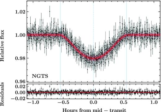
Top: 46 phase folded and detrended transits of NGTS-10b as observed by NGTS. The data have been binned in time to 5 min for clarity and then phase folded. The best-fitting transit model is overplotted in red. Bottom: Residuals after removing the best-fitting model from the top panel. The rms of the scatter out of transit is |$0.41{{\ \rm per\ cent}}$|⁠.

To help eliminate the possibility of the transit signal originating from another object, we conduct several checks for all NGTS candidates, including multicolour follow-up photometry of the transits. This enables us to measure transit depth variations that may be indicative of a false positive detection (e.g. blended eclipsing binary). We search all archival catalogues surrounding the candidate for additional stellar contamination, which may lead to transit depth dilution. We also use the centroid vetting procedure of Günther et al. (2017) to look for contamination from additional unresolved objects. This technique is able to detect sub-millipixel shifts in the photometric centre of flux during transit and can identify blended eclipsing binaries at separations <1 arcsec, well below the size of individual NGTS pixels (5 arcsec). We find no centroid variation during the transits of NGTS-10b, indicating that transit signal originates from NGTS-10.

For NGTS-10, we found one spurious detection of a neighbour in the Guide Star Catalogue v2.3 (Bucciarelli et al. 2008) and one real blended neighbour in Gaia DR2 (Gaia Collaboration 2018). We discuss these objects further in Section 3.1 and outline the treatment of the photometric contamination in Sections 3.1.1 and 4. We note that the background contaminating star falls within the photometric aperture in both the discovery photometry (this section) and the all the follow-up photometry presented in this paper (Sections 2.2 and 2.3).

2.2 Eulercam photometry

Two follow-up light curves of the transit of NGTS-10b were obtained on 2017 October 11 and 2017 December 16 with Eulercam on the 1.2 m Euler Telescope (Lendl et al. 2012) at La Silla Observatory. In October, a total of 89 images with 120 s exposure time were obtained using the Cousins I-band filter. In December, a total of 103 images with 90 s exposure time were obtained in the Gunn V band. Both observations were made in focus. The data were reduced using the standard procedure of bias subtraction and flat-field correction. Aperture photometry was performed with the phot routine from iraf. The comparison stars and the photometry aperture radius were chosen to minimize the rms in the scatter out of transit. A summary of the Eulercam observations is given in Table 1. The Eulercam light curve and best-fitting transiting exoplanet model from Section 4 are shown in Fig. 2. The undetrended follow-up Eulercam data are presented in Fig. A1.

Figure 2.

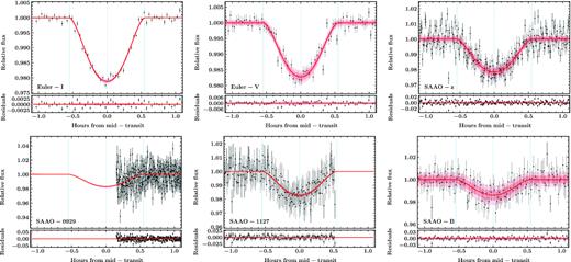
Top: From left to right, we plot the detrended follow-up light curves from Eulercam in the I and V bands on 2017 Oct 11 and 2017 Dec 16, respectively, followed by a z-band transit in from SHOCh on 2016 Nov 27. Bottom: From left to right, we plot the detrended follow-up light curves from SHOCa in the V band from nights 2017 Sept 29 to 2017 Nov 27, followed by a B-band transit on the night of 2018 Jan 29. Each light curve is overplotted with the best-fitting model from Section 4, where the red line and pink shaded regions represent the median and 1 σ and 2 σ confidence intervals of the GP-EBOP posterior transit model. The lower panel below each plot shows the residuals to the fit. The vertical blue lines highlight the start, middle, and end of each transit. The undetrended follow-up data are presented in Fig. A1.

Table 1.

A summary of the follow-up photometry of NGTS-10b transits. The FWHM and the aperture photometry radius (R_aper) values are given in units of binned pixels, if binning was applied. Both R_aper and the number of comparison stars (N_comp) were chosen to minimize the rms in the scatter out of transit (rms_OOT).

Night	Instrument	Nimages	Exptime	Binning	Filter	FWHM	Raper	Ncomp	rmsOOT	Comment
			(s)	(X × Y)		(pixels)	(pixels)		(per cent)
2016-11-27	SHOCh	630	30	4 × 4	z’	1.22	4.0	5	0.57	Full transit
2017-09-29	SHOCa	778	8	4 × 4	V	2.04	4.5	2	1.24	Partial transit
2017-10-11	Eulercam	89	120	1 × 1	I	7.32	15.0	4	0.11	Full transit
2017-11-27	SHOCa	242	30	4 × 4	V	2.1	5.0	5	0.63	Partial transit
2017-12-16	Eulercam	103	90	1 × 1	V	8.15	17.0	7	0.20	Full transit
2018-01-29	SHOCa	3278	4	4 × 4	B	1.06	2.7	1	0.79	Full transit

2.3 SHOC photometry

Four additional transit light curves of NGTS-10b were obtained using two of the three Sutherland High-speed Optical Cameras (SHOC; Coppejans et al. 2013) – SHOC’n’awe (hereafter SHOCa) and SHOC’n’horror (hereafter SHOCh). All observations were obtained with the cameras mounted on the 1 m telescope at SAAO. Observations were taken in focus with 4 × 4 binning.

The data were bias and flat-field corrected via the standard procedure using the ccdproc package (Craig et al. 2015) in python. Aperture photometry was extracted using the SEP package (Bertin & Arnouts 1996; Barbary 2016) and the sky background was measured and subtracted using the SEP background map. The number of comparison stars, aperture radius, and sky background interpolation parameters were chosen to minimize the rms in the scatter out of transit. A summary of the four follow-up light curves, two of which were complete and two of which were partial transits, is given in Table 1. The SHOCa and SHOCh light curves are shown in Fig. 2. The undetrended follow-up SHOC data are presented in Fig. A1.

2.4 TESS photometry

We inspected the TESS full frame images (FFIs) in the area surrounding NGTS-10 and find no evidence of the target nor the bright neighbour HD 42043. The TESScut³ tool returns blank FFIs for this region of sky. We checked with the TESS team, who confirmed that NGTS-10 fell in the overscan region of that particular camera. We therefore ignore TESS in the remainder of this paper.

2.5 Spectroscopy

We obtained multi-epoch spectroscopy for NGTS-10 with the HARPS spectrograph (Mayor et al. 2003) on the ESO 3.6 m telescope at La Silla Observatory, Chile, between 2016 November 3 and 2017 December 22. NGTS-10 was observed under programme IDs 098.C-0820(A) and 0100.C-0474(A) using the HARPS target ID of NG0612-2518-44284. Due to the relatively faint optical magnitude of NGTS-10 (V = 14.340 ± 0.015), we used the HARPS in the high efficiency (EGGS) mode. EGGS mode employs a fibre with a larger, 1.4 arcsec aperture, compared to standard 1.0 arcsec fibre. This allows for higher signal-to-noise spectra at slightly lower resolution of R = 85 000, compared to R = 110 000 in standard (HAM) mode.

We used the standard HARPS data reduction software (DRS) to the measure the RV of NGTS-10 at each epoch. This was done via cross-correlation with the K5 binary mask. The exposure times for each spectrum ranged between 1800 and 3600 s. The RVs are listed, along with their associated error, FWHM, bisector span, and exposure time in Table 2.

Table 2.

HARPS radial velocities for NGTS-10.

BJD	RV	RVerr	FWHM	BIS	Texp
−2450000	(km s−1)	(km s−1)	(km s−1)	(km s−1)	(s)
7696.84979	38.7113	0.0082	7.458	0.011	3600
7753.69446	38.4870	0.0091	7.446	0.078	3600
7756.82948	38.5451	0.0136	7.347	0.056	3600
7877.50407	39.6274	0.0174	7.338	−0.019	3600
8052.85264	38.5652	0.0178	7.336	−0.004	2400
8053.83621	39.4759	0.0151	7.372	0.026	2400
8054.81329	39.4719	0.0192	7.375	0.061	2400
8055.83695	38.5153	0.0077	7.513	0.005	2700
8056.78642	38.9369	0.0093	7.428	0.038	2700
8110.67686	39.6787	0.0216	7.578	0.043	1800

The RVs show a variation in phase with the photometric period detected by orion with semi-amplitude of K =|$595\, ^{+8}_{-6}$| m s⁻¹. Fig. 3 shows the phase folded RVs overplotted with the best-fitting exoplanet model from Section 4.

Figure 3.

Top: RV measurements of NGTS-10 overplotted with the best-fitting model from Section 4. The systemic velocity V_sys = 39.0931 km s⁻¹ has been subtracted from the RVs. Bottom: Residuals after the removal of the model in the upper panel. The rms of the residuals is 9.79 m s⁻¹ and is a combination of both jitter from stellar activity and instrumental noise.

To ensure that the RV signal is not caused by stellar activity, we analyse the HARPS cross-correlation functions (CCFs) using the line bisector technique of Queloz et al. (2001). We find no evidence for a correlation between the RV and the bisector spans. Fitting a line to the bisector spans in Fig. 4, we find a gradient of −0.003 ± 0.042, indicating that the RV signal is coming from orbital motion of NGTS-10 around the system barycentre rather than from stellar activity. The error on the gradient in Fig. 4 is estimated via a bootstrapping technique. We resample the bisector spans in Table 2, with replacement, a total of 1000 times. We fit a straight line to each resampled set and estimate the error on the slope as the standard deviation of the slopes from the 1000 samples.

Figure 4.

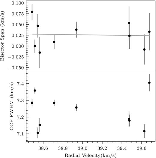
CCF bisector spans (top panel) and CCF full widths at half-maximum (bottom panel) measured from HARPS spectra plotted against the RV of NGTS-10. No correlations are found between either pair of measurements.

3 ANALYSIS

We begin this section by addressing the photometric contamination caused by a star nearby to NGTS-10 (third light). We describe the treatment of the third light in our spectroscopy in Section 3.1.1, photometry in Section 3.1.2, and then continue with the derivation of stellar properties in Sections 3.2–3.5. Finally, in Section 3.6 we hypothesize on the source of excess astrometric noise in the Gaia DR2 (Gaia Collaboration 2018) measurements of NGTS-10.

3.1 Treatment of third light

An additional object (GSC23-S3GL019224, J = 17.63) is reported in the Guide Star Catalogue v2.3 (GSC2.3) with a separation of 5.13 arcsec from NGTS-10. It is flagged as class 3 (non-stellar). As this object would be enclosed inside our photometry aperture, we consulted archival imaging of this area. Closer inspection of the photographic plates, overlaid with GSC2.3, reveals GSC23-S3GL019224 to be a spurious detection caused by the intersection of NGTS-10 and a diffraction spike of HD42043 (located 40.73 arcsec from NGTS-10, V = 9.32, Høg et al. 2000, G = 9.00, Gaia Collaboration 2016b), see Fig. 5. GSC23-S3GL01922 is not reported in 2MASS and more recently Gaia DR2 (Gaia Collaboration 2018) does not report the existence of this source. Hence, we ignore GSC23-S3GL019224 in our treatment of third light below.

Figure 5.

Archival images from the Digital Sky Survey of the area surrounding NGTS-10. HD42043 is highlighted by the yellow square, NGTS-10 is circled in cyan, and the spurious companion GSC23-S3GL019224 is marked with a magenta triangle. As can be seen, the latter appears to come from the intersection of a diffraction spike from HD42043 and NGTS-10. G-6880 is not highlighted as the source is fully encapsulated within the profile of NGTS-10. Each thumbnail is 0.75 arcmin square. North is up and East is left.

However, Gaia DR2 does report a G = 15.59 mag object (object ID: 2911987212508106880; hereafter G-6880) located 1.2 arcsec from NGTS-10 with a position angle of 334.74°. The Gaia DR2 parallax of the companion (0.297 ± 0.081 mas) places it at a much greater distance than NGTS-10 (3.080 ± 0.261 mas). We also note a significant level of astrometric noise for NGTS-10 in Gaia DR2, which we discuss in Section 6. G-6880 was also seen on the HARPS guide camera and we see evidence for it in the CCFs from our HARPS RVs. Treatment of the RV CCF and photometric contamination is discussed in the following subsections.

3.1.1 CCF analysis

A second shallow peak is occasionally visible in the CCF of our HARPS spectra (see Fig. 6). This comes from third light entering the fibre from the nearby object G-6880. The strength of the peak correlates with the instantaneous seeing at La Silla. To demonstrate that the companion is not the host of the eclipsing body, we fit a double Voigt profile to the two peaks in the CCF and measure the RV of each component.

Figure 6.

Top: 10 HARPS CCFs obtained using the K5 mask. A shallow peak can be seen near 62 km s⁻¹ in some of the CCFs. The orbital phase of each CCF is listed below the trace. Each CCF has been offset vertically by 0.15 for clarity. Bottom: The combined CCFs from the top panel. The vertical line in each plot shows the average RV of NGTS-10.

Fig. 7 shows the RVs of both peaks phased to the orbital period from the NGTS photometry. It is clear that the main CCF peak (coming from NGTS-10) is moving in phase with the photometry as expected and the second shallow peak is noisy and incoherent with the NGTS photometry. Given the above and the lack of a centroid shift measured during transit, we are certain that the photometric and RV signals are not caused by G-6880.

Figure 7.

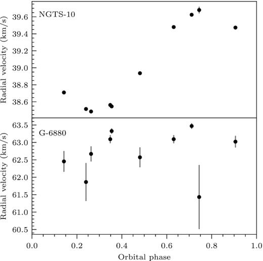
RVs of both peaks in the NGTS-10 CCFs. The top panel shows the RV signal of the main peak from NGTS-10 phased on the orbital period detected by orion. The bottom panel shows the RV signal from G-6880 phased on the same period.

3.1.2 Dilution of transit depth by third light

In order to estimate the photometric dilution caused by G-6880, we simultaneously fit the spectral energy distribution (SED) of both stars. The method is based on the analysis of NGTS-7Ab by Jackman et al. (2019). For completeness, we outline the process here. We used the PHOENIX v2 set of stellar models (Husser et al. 2013) for both stars. We initially convolved these models with the bandpasses given in Table 3 in order to generate a grid of fluxes in T_eff and log g space, assuming a Solar metallicity. This grid was then used for fitting. As the two stars are blended in all catalogue photometry except Gaia G (which is obtained through fitting the line spread function, LSF), we used the combined synthetic flux from the two stars for comparison with the observed values in all other bands.

Table 3.

Stellar properties of NGTS-10 and G-6880. The dilution factors in each bandpass are calculated as f_B/(f_A + f_B), where star A is NGTS-10 and star B is G-6880. The stellar mass, radius, and density assumed for the host are obtained from BJ1217 for a main-sequence host star with T_eff = 4400 ± 100 K. Parameters listed as Double SED and HARPS Spectra as described in Sections 3.1.2 and 3.2, respectively.

Property	Value	Source
NGTS-10 astrometric and photometric properties:
I.D.	06072933-2535417	2MASS
I.D.	2911987212510959232	Gaia DR2
RA	|$06^{\rm {h}} 07^{\rm {m}} 29{^{\rm s}_{.}}3472$|	Gaia DR2
Dec.	−25°35′41|${^{\prime\prime}_{.}}$|6268	Gaia DR2
μRA (mas yr−1)	−2.323 ± 0.343	Gaia DR2
μDec. (mas yr−1)	10.527 ± 0.395	Gaia DR2
V (mag)	14.340 ± 0.015a	APASS
B (mag)	15.274 ± 0.044a	APASS
g (mag)	14.780 ± 0.040a	APASS
r (mag)	13.980 ± 0.050a	APASS
i (mag)	13.637 ± 0.015a	APASS
G (mag)	14.260 ± 0.005	Gaia DR2
NGTS (mag)	13.626 ± 0.010a	NGTS photometry
J (mag)	12.392 ± 0.026a	2MASS
H (mag)	11.878 ± 0.028a	2MASS
K (mag)	11.728 ± 0.025a	2MASS
W1 (mag)	11.644 ± 0.024a	WISE
W2 (mag)	11.672 ± 0.022a	WISE
G-6880 astrometric and photometric properties:
I.D.	2911987212508106880	Gaia DR2
RA	|$06^{\rm {h}} 07^{\rm {m}} 29{^{\rm s}_{.}}3118$|	Gaia DR2
Dec.	−25°35′40|${^{\prime\prime}_{.}}$|6118	Gaia DR2
μRA (mas yr−1)	−1.120 ± 0.219	Gaia DR2
μDec. (mas yr−1)	9.671 ± 0.161	Gaia DR2
G (mag)	15.593 ± 0.005	Gaia DR2
Dilution parameters:
δNGTS	|$0.22\, ^{+0.03}_{-0.02}$|	Double SED
δi	|$0.19\, ^{+0.03}_{-0.02}$|	Double SED
δV	|$0.30\, ^{+0.03}_{-0.02}$|	Double SED
δB	|$0.42\, ^{+0.04}_{-0.03}$|	Double SED
δz	|$0.18\, ^{+0.03}_{-0.02}$|	Double SED
σf	|$0.0498\, ^{+0.048}_{-0.030}$|	Double SED
NGTS-10 derived properties:
Teff (K)	4400 ± 100	Double SED
S	0.287 ± 0.02 × 10−20	Double SED
Av (mag)	|$0.0067\, ^{+0.0174}_{-0.0098}$|	Double SED
Spectral type	K5V	Double SED
Age (Gyr)	10.4 ± 2.5	Double SED
Teff (K)	4600 ± 150	HARPS Spectra
[M/H]	−0.02 ± 0.12	HARPS Spectra
log (g)	4.5 ± 0.2	HARPS Spectra
vsin i⋆ (km s−1)b	≤4.0 ± 0.6	HARPS Spectra
γRV (km s−1)	|$39.0931\, ^{+0.0054}_{-0.0057}$|	HARPS Spectra
log R’HK	−4.70 ± 0.19	HARPS Spectra
Ms (M⊙)	0.696 ± 0.040	B1217
Rs (R⊙)	0.697 ± 0.036	B1217
log g	4.595 ± 0.019	B1217
Prot (d)	17.290 ± 0.008	NGTS photometry
G-6880 derived properties:
Teff (K)	|$6263\, ^{+206}_{-212}$|	Double SED
S	|$0.178\, ^{+0.0070}_{-0.0044}\times 10^{-20}$|	Double SED
log g	4.0 ± 0.26	Double SED
Av (mag)	|$0.0366\, ^{+0.074}_{-0.040}$|	Double SED

Note. 2MASS (Skrutskie et al. 2006); APASS (Henden & Munari 2014); WISE (Wright et al. 2010); Gaia (Gaia Collaboration 2016a); B1217 = Boyajian et al. (2012), Boyajian et al. (2017).

a

Note that all catalogue photometry of NGTS-10 is blended with G-6880, except for Gaia G.

b

v_macro = 0 km s⁻¹.

Gaia DR2 reports an astrometric noise excess of 2.1518 mas for NGTS-10. The Gaia DR2 release notes warn that the parallax measurements are compromised when the astrometric noise excess exceeds 2 mas, hence we chose to ignore the Gaia parallax and instead fit for T_eff, the extinction A_V, and the scale factor S (S = R²/D², where R and D are the radius and distance of the star, respectively) for each star.

When fitting for A_V we used the extinction law of Fitzpatrick (1999) with the improvements of Indebetouw et al. (2005). We also fit for log g of G-6880 but fixed the log g of NGTS-10 at the value determined from our stellar spectra described in Section 3.2. Finally we fit an uncertainty inflation term σ_f, which is used to inflate the uncertainties on observed fluxes and account for potentially underestimated errors.

When fitting, we required the synthetic Gaia G-band flux for each source to match the observed values. This was achieved via a Gaussian prior for each source. We required the extinction of G-6880 to be greater than that of NGTS-10, to match our expectations from their relative distances. In order to fully explore the posterior parameter space, we used emcee (Foreman-Mackey et al. 2013) to generate a Markov Chain Monte Carlo (MCMC) process using 100 walkers for 10 000 steps, conservatively taking the final 1000 steps to sample the distribution. As the parameters derived from the SED fit are model dependent, we inflate the formal error bars by a factor of 2 to account for potential differences in stellar models.

To calculate the dilution of the background source in each of the filters given in Table 1 (and in the NGTS filter), we used the posterior distribution directly from our SED fitting. Each SED model was used to generate synthetic fluxes in each filter, which were then used to calculate the dilution. The resulting dilution values and stellar parameters are given in Table 3 and the SEDs are plotted in Fig 8. We note that the dilution factors calculated here are lower limits based on the completeness of Gaia DR2.

Figure 8.

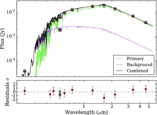
Top: Double SED fit to the available catalogue photometry of NGTS-10 and G-6880. Note, that the two stars are only resolved in the Gaia G band. The SED of NGTS-10 is plotted in green, G-6880 is plotted in magenta, and the combined SEDs of both stars are plotted in black. Cyan markers represent the observed catalogue photometry, while the red markers are our combined synthetic photometry. The Gaia points are plotted with square markers, all others are circles. We have inflated the cyan marker size as they were often hidden behind the red markers. Bottom: The residuals to the double SED fit versus wavelength. The red circles represent the difference between our catalogue and synthetic photometry. The Gaia photometric points are given as cyan squares.

3.2 Stellar properties

The HARPS spectra were ordered by increasing seeing. We combined the six with the sharpest seeing and the least evidence of contamination by G-6880 into a higher SNR spectrum. Using methods similar to those described by Doyle et al. (2013), we determined values for the stellar effective temperature T_eff, surface gravity log g, stellar metallicity [Fe/H], and the projected stellar rotational velocity vsin i_⋆. In determining vsin i_⋆, we assumed a zero macroturbulent velocity, as it is below that of thermal broadening (Gray 2008). Hence, vsin i_⋆ = 4.0 ± 0.6 km s⁻¹ is an upper limit. Lithium is not seen in the spectra. We find T_eff = 4600 ± 150 K and log g = 4.5 ± 0.2 which are consistent with our double SED fit from Section 3.1.2. We note that the T_eff obtained from the combined spectroscopy has a relatively large uncertainty due to the low SNR of the combined spectrum (SNR ∼ 30) and the weak Balmer line. If we adopt the effective temperature for NGTS-10 from the Section 3.1.2, the log g value decreases to 4.3 ± 0.2, but is still consistent with a main-sequence star.

In order to obtain a consistent set of stellar parameters for the third light calculation and the global analysis in Section 4, we adopt the effective temperature of NGTS-10 from the double SED fit in Section 3.1.2. Given the excess astrometric noise for NGTS-10, we also ignore the Gaia distance. Without the distance, we are forced to assume that the star is on the main sequence. If instead the Gaia parallax and the distance (325 ± 29 pc) were correct, our fitted scaling factor S from Section 3.1.2 would imply a stellar radius of 0.77 ± 0.07 R_⊙, which is still consistent with a main-sequence star within the uncertainties. Additionally, as seen below in Section 3.3 the host star’s kinematics show that it is consistent with a thin disc object regardless of whether we trust the Gaia DR2 parallax or not, which strengthens our assumption of a main-sequence host. Finally, we obtain main-sequence mass and radius for a 4400 ± 100 K star using the relations from Boyajian et al. (2012, 2017). We list the stellar parameters in Table 3.

3.3 Kinematics

To check whether NGTS-10 is consistent with belonging to the Galactic thin disc, we calculated its kinematics using the stellar parameters from Table 3. We compared the solution to the selection criteria of Bensby, Feltzing & Lundström (2003) and calculated the thick disc to thin disc (P_thick/P_thin) relative probability. As a check, this was repeated using the slightly larger stellar radius (0.77 ± 0.07 R_⊙) implied by the Gaia parallax. We found that for both scenarios, NGTS-10 was more likely to belong to the thin disc (P_thick < 0.1 × P_thin) than the thick disc. This is also shown in the Toomre diagram in Fig. 9, supporting our assumption that the host star is on the main sequence.

Figure 9.

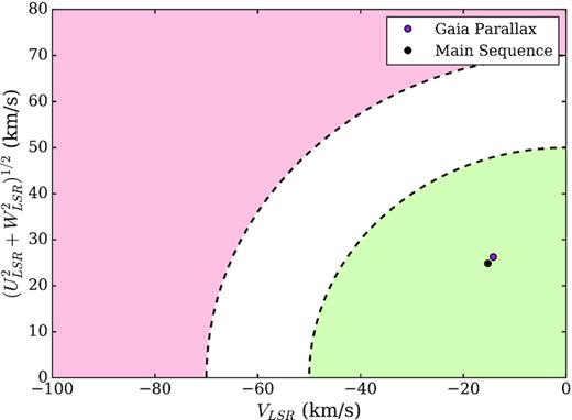
Toomre diagram for NGTS-10 for our two scenarios. The purple marker corresponds to the solution when we use the Gaia parallax and the black marker is when we assume NGTS-10 is on the main sequence. The green and red regions represent the expected total velocity distributions for the thin and thick disc, respectively, using the values from Bensby, Feltzing & Oey (2014). The white area is a region of intermediate probability. Note that in both scenarios, NGTS-10 is well within the expected velocity range for a thin disc source.

3.4 Stellar activity and rotation

We verified the stellar rotation period by calculating the generalized autocorrelation function (G-ACF) of the NGTS photometric time series (Kreutzer et al., in preparation). The ACF is a proven method for extracting stellar variability from photometric light curves (as in McQuillan, Mazeh & Aigrain 2014), and this generalization allows analysis of irregularly sampled data. This method has been used on NGTS data to successfully extract rotation periods from a large numbers of stars within the Blanco 1 open cluster (Gillen et al. 2019).

We first binned the time series to 20 min, giving 2432 data points. As the G-ACF does not return an error on the rotation period directly, we employ a bootstrapping technique. We randomly select 2000 data points from the binned NGTS time series and run the G-ACF analysis. This was repeated 1024 times, giving a rotation period and error of 17.290 ± 0.008 d, where the error is the standard deviation in the periods from the 1024 runs, divided by |$\sqrt{1024}$|⁠.

Fig. 10 shows this clear periodic signal. This period was verified to be unique for objects within the vicinity of NGTS-10 on the NGTS CCD, providing strong evidence that this is not a systematic feature. We note that the rotation period of 17.290 ± 0.008 implies a stellar rotation velocity of 2.04 ± 0.11 km s⁻¹which is smaller than the 4.0 ± 0.6 upper limit quoted in Section 3.2. Extrapolation of the (Doyle et al. 2014) calibration suggests a value for macroturbulence could be v_macro∼3.5 km s⁻¹, which would give a vsin i_⋆∼2.0 km s⁻¹, which is in line with the photometric rotation period above. This high value of macroturbulence, is supported by the relation used by the Gaia-ESO Survey which gives v_macro=3.8 km s⁻¹. Additionally, we find evidence for line core emission in the Ca ii H and K lines with an activity index of log R’_HK = −4.70 ± 0.19. This evidence for stellar activity may additionally support the case for a non-zero macroturbulent velocity.

Figure 10.

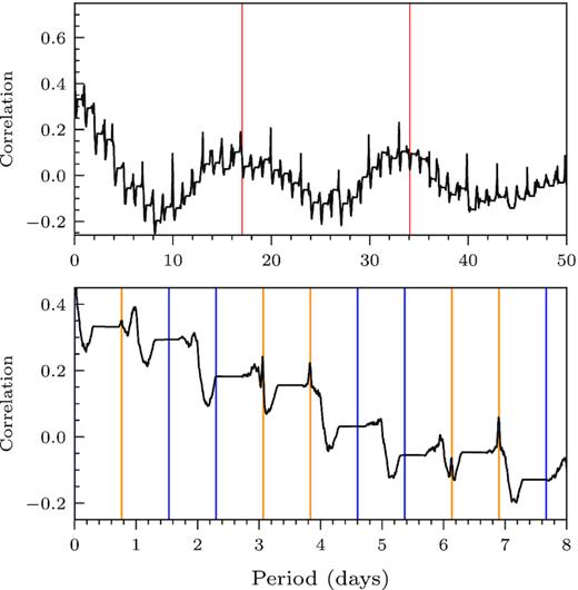
Top: The generalized autocorrelation function (G-ACF) of the NGTS light curve. The red lines highlight the 17.290 ± 0.008 d periodicity detected. Bottom: Zooming further in on the G-ACF reveals the planet transit signal at P = 0.76689 d as predicted. The vertical lines show clear periodic increases in the autocorrelation. Orange lines indicate we observe a transit, and blue lines indicate a gap in the data.

3.5 Stellar age

We place constraints on the age of the host star using the Bayesian fitting process described in Maxted, Serenelli & Southworth (2015), and which is available as the open source bagemass⁴ code. bagemass uses the GARSTEC models of Weiss & Schlattl (2008), as computed by Serenelli et al. (2013), and works in [log (L_star), T_eff].

We perform a stellar model fit using all three sets of model grids available within bagemass, deriving age estimates that agree within 1σ. In Fig. 11, we show the posterior probability distribution for the fit to one of those grids. We adopt a final age of 10.4 ± 2.5 Gyr, calculating as the weighted average of the three fits, which is consistent with the age of the thin disc (8.8 ± 1.7 Gyr; del Peloso et al. 2005) within the uncertainties.

Figure 11.

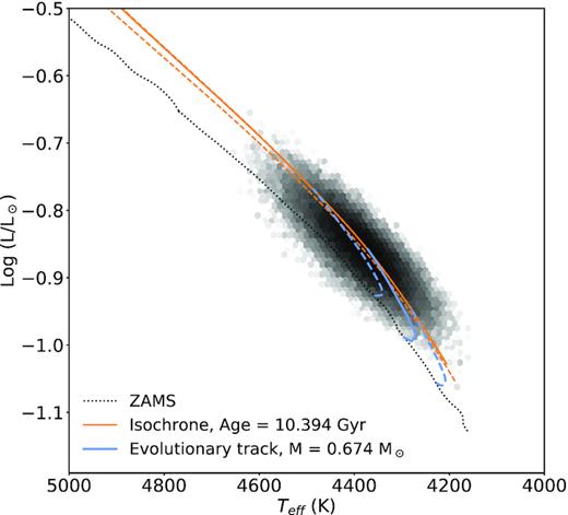
The results from stellar model fitting using bagemass, showing the best-fitting stellar models and the posterior probability distribution of the MCMC fitting process, the colour scale of which represents the density of points. The ZAMS is shown as a dotted black line. The solid blue line is the best-fitting stellar evolutionary tracks, with the blue dashed lines representing evolutionary tracks for the 1σ limits on stellar mass. The solid orange line is the stellar isochrone, with the orange dashed lines representing isochrones for the 1σ limits on stellar age.

3.6 Analysis of Gaia scan angles

Gaia DR2 quotes an astrometric noise of 2.1518 mas for NGTS-10 but only 0.0644 mas for G-6880, which was initially puzzling. With the current data release, we are unable to analyse the astrometric data from individual scans separately to draw more detailed conclusions. Below we hypothesize on what may be happening. Gaia DR2 contains 332 and 122 astrometric measurements of NGTS-10 and G-6880, respectively. Of these, 320 and 122 are flagged as being good, respectively. This discrepancy between the numbers of astrometric measurements for the two sources may point to G-6880 being unresolved in 62 per cent of scans and could help explain the source of the astrometric noise excess. We inspected 89 scan angles available via Gost and measured the angular offsets between the position angle of the NGTS-10/G-6880 blended pair (334.74°) and each individual scan angle. The distribution of angular offsets is shown in Fig. 12. Propagating our assumption above, we draw a line at 62 per cent on the histogram in the lower panel of Fig. 12, indicating that once the scan angle is within 60° of the blend PA, the two sources appear to become confused. We plan to revisit this issue when the individual data astrometric measurements become available in Gaia DR4.

Figure 12.

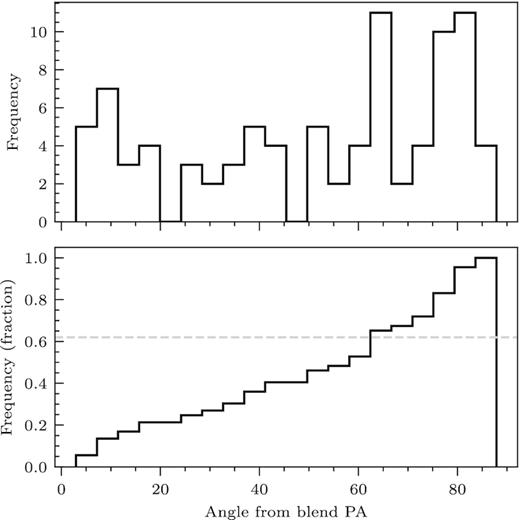
Top: Histogram showing the distribution of Gaia scan angles with respect to the position angle of the NGTS-10 and G-6880 blend. Gaia scanned across the blend over a range of angles from coplanar to perpendicular. Bottom: A cumulative frequency distribution of the data in the top panel. The dashed grey line shows the fraction of measurements where Gaia measures astrometry for NGTS-10 only. To explain the discrepancy between the numbers of measurements of the two sources in the blend, we hypothesize that once the scan angle of Gaia is within approximately 60° of the blend PA, the two sources appear to become confused.

4 GLOBAL MODELLING

We modelled the NGTS and follow-up data with GP-EBOP (Gillen et al. 2017) to determine fundamental and orbital parameters of NGTS-10b. The full data set comprises the NGTS discovery light curve (containing 46 transits), six follow-up transit light curves (in four photometric bands), and 10 HARPS RVs. GP-EBOP comprises a central transiting planet and eclipsing binary model, which is coupled with a Gaussian process (GP) model to simultaneously account for correlated noise in the data, and uses MCMC to explore the posterior parameter space. Limb darkening is treated using the analytic prescription of Mandel & Agol (2002) for the quadratic law.

Each light-curve bandpass possesses its own stellar variability and each transit observation possess its own atmospheric/instrumental noise properties, which will affect the apparent transit shape and hence the inferred planet parameters. To account for this, GP-EBOP simultaneously models the variability and systematics using GPs, at the same time as fitting the planet transits, which gives a principled framework for propagating uncertainties in the noise modelling through into the planet posterior parameters. We chose a Matern-32 kernel for all light curves given the reasonably low level of stellar variability but clear instrument systematics and/or atmospheric variability. Limb darkening profile priors were generated with LDtk (Parviainen & Aigrain 2015) assuming the T_eff, log g, and [Fe/H] values from the double SED fit given in Table 3. We placed Gaussian priors on the dilution factors in each photometry band using the values in Table 3.

The NGTS data were binned to 5 min and the GP-EBOP model binned accordingly. The SAAO B-band light curve was binned to 1 min cadence but we opted not to integrate the GP-EBOP model given the short resulting cadence. All other light curves were modelled at the cadences reported in Table 1.

Given the sparse RV coverage (10 data points over 400 d), we opted not to include a GP noise model in the GP-EBOP RV model, and instead incorporated a white noise jitter term, under penalty, that was added in quadrature to the observational uncertainties. Given the limited information contained within the RV data and the extremely short period, we assumed a circular Keplerian orbit for the planet. We tried fitting the RVs with a linear drift in time but found a zero slope (8.0 ± 8.6 m s⁻¹) and a reduced χ² < 0 (overfitting), so we opted to exclude the linear drift from the RV fit in the final MCMC run. Using the method of Suárez Mascareño et al. (2017) for a star of log R’_HK = −4.70 ± 0.19, we calculate a stellar jitter of 2.9 m s⁻¹. The rms of the RV residuals (see lower panel in Fig. 3) is 9.79 m s⁻¹ and the average error on each RV measurement is 14 m s⁻¹. Hence, the precision of the RV measurements is limited by the instrumental performance and not by stellar jitter.

We performed 200 000 MCMC steps with 300 walkers, discarding the first 100 000 steps as a conservative burn in. The resulting chains yielded posterior values for the fundamental and orbital planet parameters, which are reported in Table 4. The posteriors can be seen in Fig. 13. The grazing nature of the system resulted in skewed distributions of (R_p + R_s)/a, R_p/R_s, and |$\cos \, i$|⁠, hence we extracted the best-fitting values and their uncertainties using the mode and full width at half-maximum of each distribution. We find that NGTS-10b has a mass and radius of M_p = |$2.162\, ^{+0.092}_{-0.107}$|M_J and R_p = |$1.205\, ^{+0.117}_{-0.083}$|R_J, and orbits its host star in 0.7668944 ± 0.0000003 d at a distance of 0.0143 ± 0.0010 au.

Figure 13.

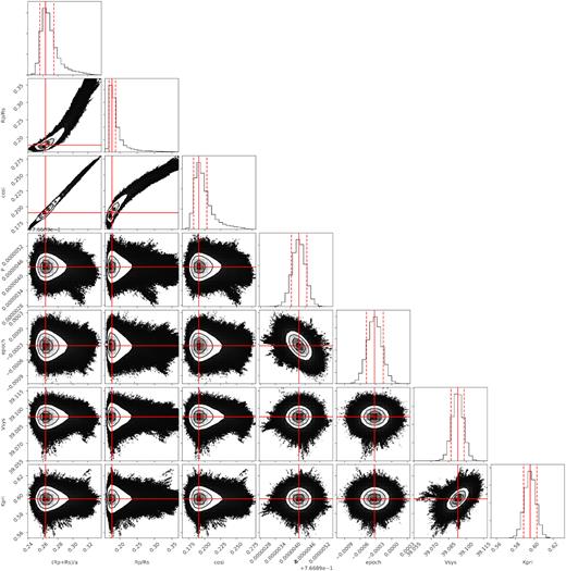
MCMC posterior distributions. A total of 300 walkers and 200 000 steps were used in this fit. We plot the MCMC chain for the final 100 000 steps showing every 500th element only. The solid red lines mark the mode of each parameter’s distribution while the dashed red lines mark the full width at half-maximum. We use the mode as the grazing nature of the system causes the distributions of (R_p + R_s)/a, R_p/R_s, and |$\cos \, i$| to be skewed. Both the median and mean of the distributions overestimate the parameters and do not represent the peak of each distribution.

Table 4.

Best-fitting and derived parameters from the global modelling of NGTS-10b.

Parameter	Symbol	Unit	Value
Transit parameters
Sum of radii	|$( {R}_{\rm {s}}+ {R}_{\rm {p}})/ {a}$|	–	|$0.2637\, ^{+0.0105}_{-0.0081}$|
Radius radio	|${R}_{\rm {p}}/ {R}_{\rm {s}}$|	–	|$0.1765\, ^{+0.0110}_{-0.0070}$|
Cosine inclination	cos i	–	|$0.1890\, ^{+0.0142}_{-0.0071}$|
Impact parameter	b	–	|$0.8523\, ^{+0.03158}_{-0.0197}$|
Epoch	T0	HJD	2457518.84377 ± 0.00017
Period	P	d	0.7668944 ± 0.0000003
Eccentricity	e	–	0 (fixed)
Dilution NGTS	δNGTS	–	|$0.210\, ^{+0.021}_{-0.027}$|
Dilution I band	δI	–	0.200 ± 0.026
Dilution V band	δV	–	0.297 ± 0.026
Dilution z band	δz	–	0.193 ± 0.034
Dilution B band	δB	–	|$0.398\, ^{+0.051}_{-0.045}$|
Radial velocity parameters
Systemic velocity	Vsys	km s−1	39.0931 ± 0.0057
RV semi-amplitude	K	km s−1	|$0.5949\, ^{+0.0077}_{-0.0063}$|
Planet parameters:
Planet mass	Mp	MJ	|$2.162\, ^{+0.092}_{-0.107}$|
Planet radius	Rp	RJ	|$1.205\, ^{+0.117}_{-0.083}$|
Planet density	ρp	g cm−3	|$1.430\, ^{+0.354}_{-0.404}$|
Semimajor axis	a	au	0.0143 ± 0.0010
Semimajor axis	a/Rs	–	|$4.447\, ^{+0.123}_{-0.141}$|
Transit duration	T14	h	1.091 ± 0.019
Equilibrium temp.	Teq	K	|$1332\, ^{+49}_{-54}$|

5 TIDAL MODELLING

Owing to the ultrashort orbital period of NGTS-10b, it is likely to undergo strong tidal interactions with its host star, and ultimately undergo orbital decay. We therefore model the tidal interactions in the system to constrain the remaining lifetime of the planet. We adopt the tidal evolution model of Brown et al. (2011), which implements the equilibrium tide theory of Eggleton, Kiseleva & Hut (1998) as parametrized by Dobbs-Dixon, Lin & Mardling (2004).

We define a set of values for the stellar tidal quality factor |$Q^{\prime }_{s}$|⁠, {|$\log Q^{\prime }_{\rm s}$||5, 6, 7, 8, 9, 10} to explore for the system; these are assumed to be constant with time. It is very likely that the value of |$Q^{\prime }_{s}$| evolves over time as the structure of the star changes, particularly the radial extent of its radiative and convective regions, which are known to affect the efficiency of tidal dissipation. For example, Bolmont & Mathis (2016) found that young stars are much more dissipative than main-sequence stars owing to their extended convective envelopes. However, detailed modelling of the dynamical tide (e.g. following Ogilvie & Lin 2007), which would give a more accurate picture of the future evolution of this system, is beyond the scope of this paper.

We set the planetary tidal quality factor as constant, |$\log Q^{\prime }_{\rm p}$| = 8, as Brown et al. found this parameter to have a negligible effect on semimajor axis evolution. Without knowledge of the planet’s interior structure, estimating the moment of inertia constant is difficult. As the density of NGTS-10b (⁠|$1.430\, ^{+0.354}_{-0.404}$| g cm⁻³) is similar to that of Jupiter (1.33 g cm⁻³), we assume the Jovian moment of inertia 0.2756 ± 0.006 from Ni (2018). Alvarado-Montes & García-Carmona (2019) showed that such an assumption can lead to misrepresentation of the true tidal evolution of a system, and that the physical evolution of giant planets plays a key role in determining the strength of tidal interactions in hot Jupiter systems. However, they also note that the tidal dissipative properties of exoplanets and stars are poorly defined, that constant properties can be a reasonable approximation given the lack of information on interior properties.

For each value of |$\log Q^{\prime }_{\rm s}$|⁠, we draw 1000 random samples from Gaussian distributions in system age, semimajor axis, eccentricity (to avoid divide-by-zero errors, we assume a negligible but non-zero eccentricity of 10⁻⁶), and stellar rotation frequency. Each Gaussian is centred on the model value from Table 4 and has a width equal to the listed 1σ uncertainty. Where the uncertainty is asymmetric, a skewed Gaussian was used.

For each set of random samples, we use a fourth-order Runge–Kutta integrator (adapted from algorithms in Press et al. 1992) to integrate the set of equations (1), (6), (7), and (12) from Brown et al. (2011) forwards from the sampled age until twice the host star’s estimated main-sequence lifetime has elapsed, or until the planet reaches the Roche limit, which we define as

$$\begin{eqnarray} a_{\rm Roche} = 2.46{R_{\rm p}}\left(\frac{{M_{\rm s}}}{{M_{\rm p}}}\right)^{1/3}. \end{eqnarray}$$

(1)

Figs 14 and 15 show the resulting ensemble evolutionary traces for semimajor axis and stellar rotation period, respectively. Also plotted are ‘baseline’ traces which use the values from Table 4 as their starting point. For |$\log Q^{\prime }_{\rm s}$| = 10, i.e. very inefficient dissipation and thus very weak tidal forces, we find that many of the traces reach maximum runtime rather than ending at the Roche limit. Fig. 16 plots histograms of the remaining time to reach the Roche limit for the different values of |$\log Q^{\prime }_{\rm s}$|⁠. For values of |$\log Q^{\prime }_{\rm s}$| more consistent with those found for other hot Jupiters, we find that the planet reaches the Roche limit on time-scales of the order Myr (⁠|$\log Q^{\prime }_{\rm s}$| = 6) to hundreds of Myr (⁠|$\log Q^{\prime }_{\rm s}$| = 8).

Figure 14.

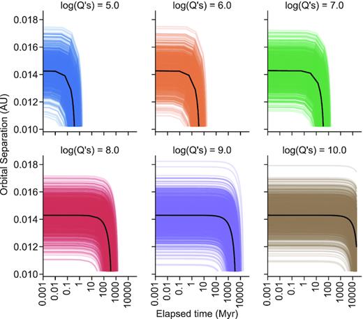
Semimajor axis as a function of elapsed time for different values of |$\log Q^{\prime }_{\rm s}$|⁠. In each panel, each coloured line represents a possible history based on a set of parameters drawn randomly from distributions based on the observed parameters. The black line in each panel denotes the evolution taking the observed parameters at face value. The tracks cut-off when the planet reaches the Roche limit, or twice the estimated main-sequence lifetime of the host star.

Figure 15.

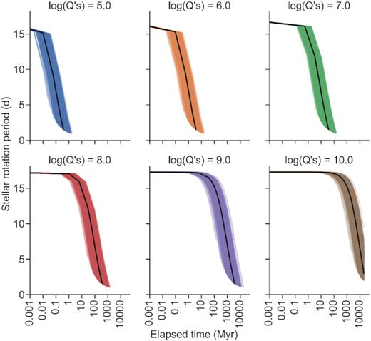
Stellar rotation period as a function of elapsed time for different values of |$\log Q^{\prime }_{\rm s}$|⁠. Format is as for Fig. 14.

Figure 16.

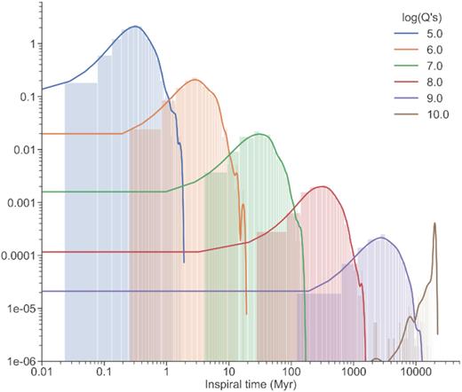
Histograms of inspiral time for different values of |$\log Q^{\prime }_{\rm s}$|⁠. As the efficiency of tidal dissipation decreases, the spread in modelled inspiral time increases. Note that the y-axis is log-formatted for display purposes.

In all cases, the host star is spun up during the tide-driven evolution of the planet’s orbit. For the ‘baseline’ traces, the stellar rotation period when the planet reaches the Roche limit is between 1.4 and 1.9 d. The full range of final stellar rotation periods is 1.0 d ≤P_rot ≤ 9.4 d, though we note that this includes traces that halt at the maximum runtime rather than the Roche limit, and have thus experienced less evolution of the system parameters.

6 DISCUSSION

Our observations and modelling show that NGTS-10 hosts a hot Jupiter with the shortest orbital period yet found. It orbits its K5 host star with a period of only 18.4 h (0.7668944 ± 0.0000003 d). We have determined the mass (⁠|$2.162\, ^{+0.092}_{-0.107}$| M_J) and radius (⁠|$1.205\, ^{+0.117}_{-0.083}$| R_J) of the planet to better than 5 per cent and 10 per cent precision, respectively. Fig. 17 shows NGTS-10b in the context of the current population of transiting hot Jupiters with precisely determined masses and radii (≤20 per cent precision). The top panel highlights NGTS-10b as an extreme object, pushing the bounds of planetary mass/period parameter space. NGTS-10b orbits its host star at only |$4.447\, ^{+0.123}_{-0.141}$| stellar radii (or 1.462 ± 0.179 Roche radii).

Figure 17.

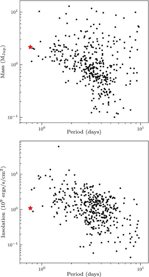
Top: Planet mass versus orbital period. Bottom: Received insolation versus orbital period. In each plot, we show planets with masses and radii determined to 20 per cent precision or better, periods <10 d and masses in the range 0.1–|$13\, M_{\mathrm{Jup}}$|⁠. Error bars are excluded for clarity and NGTS-10b is highlighted with a red star.

Hot Jupiters are typically prime candidates for atmospheric characterization. The close proximity to their host star increases the level of reflected light and raises their equilibrium temperatures leading to increased thermal emission. This in turn permits atmospheric characterization via secondary eclipse and phase curve measurements. Shporer et al. (2019) recently used this technique to measure the low albedo and the inefficient redistribution of energy in the atmosphere of WASP-18b. Atmospheric characterization is also possible via transmission spectroscopy. The transmission spectroscopy signal strength is increased for planets with larger atmospheric scale heights (H) and smaller host star radii. A planet’s atmospheric scale height is driven by its equilibrium temperature and surface gravity. Although NGTS-10b is the shortest period Jupiter yet discovered, the host star is relatively cool (T_eff = 4400 K) which leads to a lower insolation (see bottom panel of Fig. 17 and Table 5) and a lower equilibrium temperature when compared to other USP hot Jupiters. We calculate a fairly typical scale height of H = 135 km for NGTS-10b but given it orbits a relatively small K5V star, the transmission spectroscopy signal strength is comparable to that of the well-studied USP hot Jupiters WASP-18b and WASP-103b. Atmospheric characterization of NGTS-10b in the optical will be challenging given the faintness of the host star (V = 14.3). However, in the infrared the host star is much brighter (H = 11.9), this combined with the expected strength of its transmission spectroscopy signal makes NGTS-10b a potential candidate for atmospheric characterization using JWST and NIRSpec.

Table 5.

Orbital parameters of the currently known USP hot Jupiters.

Name	Period	Semimajor	a/Rstar	a/RRoche	Insolation	Reference
	(d)	axis (au)			(× 109 ergs s−1 cm−2)
NGTS-10b	0.7668944 ± 0.0000003	0.0143 ± 0.0010	|$4.447\, ^{+0.123}_{-0.141}$|	1.462 ± 0.179	1.091 ± 0.214	This work
NGTS-6b	0.882058 ± 0.000001	0.01662 ± 0.00050	3.1268 ± 0.3789	1.1044 ± 0.2149	0.723 ± 0.189	Vines et al. (2019)
WASP-18b	0.941450 ± 0.000001	0.02030 ± 0.00700	3.3838 ± 1.1742	2.8370 ± 1.0109	8.470 ± 5.884	Stassun, Collins & Gaudi (2017)
WASP-19b	0.788838989 ± 0.000000040	0.01634 ± 0.00024	3.4996 ± 0.0758	1.0481 ± 0.0392	4.450 ± 0.298	Wong et al. (2016)
WASP-43b	0.813475 ± 0.000001	0.01420 ± 0.00040	5.0891 ± 0.3683	1.8735 ± 0.1637	0.821 ± 0.191	Hellier et al. (2011)
WASP-103b	0.925542 ± 0.000019	0.01985 ± 0.00021	2.9724 ± 0.1121	1.1725 ± 0.0631	8.944 ± 1.155	Gillon et al. (2014)
KELT-16b	0.9689951 ± 0.0000024	0.02044 ± 0.00026	3.2318 ± 0.1575	1.6032 ± 0.1042	8.209 ± 0.849	Oberst et al. (2017)
HATS-18b	0.83784340 ± 0.00000047	0.01761 ± 0.00027	3.7125 ± 0.2151	1.3797 ± 0.1108	4.046 ± 0.583	Penev et al. (2016)

A major problem with investigations of tidal evolution is placing constraints on |$Q^{\prime }_{\rm s}$|⁠. Previous studies have attempted to do this on a system by system basis (e.g. Brown et al. 2011; Penev et al. 2016), but a recent paper by Penev et al. (2018) described a simple relationship between |$Q^{\prime }_{\rm s}$| and the tidal forcing period, which itself is a simple function of the orbital and stellar rotation periods. We use equations (1) and (2) of Penev et al. (2018) to calculate a value of |$Q^{\prime }_{\rm s}$| = 2 × 10⁷ for NGTS-10. Based on this, we estimate a median inspiral time of 38 Myr for NGTS-10b from the distribution for |$\log Q^{\prime }_{\rm s}$| = 7 in Fig. 16.

However, recent work by Heller (2019) predicted that we are unlikely to observe tidally driven orbital decay in systems such as NGTS-10b owing to extremely inefficient tidal dissipation in the convective envelope of main-sequence, Sun-like stars. Heller (2019) also demonstrated that the pile-up of hot Jupiters around 0.05 au could be reproduced by a combination of the dynamical tide and type-II planet migration. NGTS-10b’s location at much shorter semimajor axis thus suggests either an old age, supporting the bagemass prediction, or stronger tides than are typical for a star of this type.

If we assume that NGTS-10b is likely to have a decaying orbit, it is interesting to consider on what time-scale might we be able to detect changes in orbital period or transit times. We use equation (27) of Collier Cameron & Jardine (2018) to determine the quadratic change in transit time on human-observable time-scales of order one decade. We predict a change of 2 s over 5 yr, and 7 s over 10 yr, assuming |$Q^{\prime }_{\rm s}$| = 2 × 10⁷ (see Fig. 18). NGTS-10b therefore joins WASP-19 and HATS-18 as reasonable candidates for the direct measurement of orbital period decay over the coming years. We note that our current precision on T₀ is approximately 15 s. Therefore, detecting the comparably small variation in transit timing (7 s) will require higher cadence and higher quality transit observations if it is to be measured accurately. We also note that an ongoing RV survey would also be needed to rule out the influence of additional longer period planets in the system.

Figure 18.

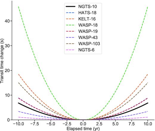
Change in transit time as a function of elapsed time over a 20 yr baseline for NGTS-10b, assuming a value of |$Q^{\prime }_{\rm s}$| = 2 × 10⁷. Also plotted are the equivalent curves for the other currently known USP hot Jupiters listed in Table 5.

7 CONCLUSIONS

We report the discovery of the shortest period hot Jupiter to date, NGTS-10b. We have determined the planetary mass and radius to better than 5 per cent and 10 per cent precision, respectively. NGTS-10 is determined to be a K5 main-sequence star with an effective temperature of 4400 ± 100 K. Our tidal analysis determined a quality factor |$Q^{\prime }_{\rm s}$| = 2 × 10⁷ for NGTS-10 and a median inspiral time of 38 Myr for NGTS-10b. We calculate a potentially measurable transit time change of 7 s over the coming decade. We aim to obtain high-precision transit observations over the coming years to directly measure the efficiency of the tidal dissipation. Due to the blended nature of the system, with a contaminating source, the precise distance to NGTS-10 remains uncertain. Using data from future Gaia releases, we plan to revisit this outstanding issue.

SUPPORTING INFORMATION

shoc_photometry_B-band.dat

shoc_photometry_V-band_20171127.dat

shoc_photometry_z-band.dat

ngts_photometry.dat

shoc_photometry_V-band_20170929.dat

eulercam_photometry_I-band.dat

eulercam_photometry_V-band.dat

harps_radial_velocities.dat

Please note: Oxford University Press is not responsible for the content or functionality of any supporting materials supplied by the authors. Any queries (other than missing material) should be directed to the corresponding author for the article.

ACKNOWLEDGEMENTS

Based on data collected under the NGTS project at the ESO La Silla Paranal Observatory. The construction of the NGTS facility was funded by the University of Warwick, the University of Leicester, Queen's University Belfast, the University of Geneva, the Deutsches Zentrum für Luft- und Raumfahrt e.V. (DLR; under the ‘Großinvestition GI-NGTS’), the University of Cambridge, and the UK Science and Technology Facilities Council (STFC; project reference ST/M001962/1). The NGTS facility is operated by the consortium institutes with support from STFC under projects ST/M001962/1 and ST/S002642/1. This paper uses observations made at the South African Astronomical Observatory (SAAO). The contributions at the University of Warwick by PJW, RGW, DLP, DJA, BTG, and TL have been supported by STFC through consolidated grants ST/L000733/1 and ST/P000495/1. Contributions at the University of Geneva by FB, BC, LDN, ML, OT, and SU were carried out within the framework of the National Centre for Competence in Research ‘PlanetS’ supported by the Swiss National Science Foundation (SNSF). The contributions at the University of Leicester by MRG and MRB have been supported by STFC through consolidated grant ST/N000757/1. EG gratefully acknowledges support from the David and Claudia Harding Foundation in the form of a Winton Exoplanet Fellowship. CAW acknowledges support from the STFC grant ST/P000312/1. TL was also supported by STFC studentship 1226157. MNG acknowledges support from MIT’s Kavli Institute as a Juan Carlos Torres Fellow. DJA acknowledges support from the STFC via an Ernest Rutherford Fellowship (ST/R00384X/1). SLC acknowledges support from the STFC via an Ernest Rutherford Fellowship (ST/R003726/1). JSJ acknowledges support by FONDECYT grant 1161218 and partial support by CATA-Basal (PB06, CONICYT). JIV acknowledges support of CONICYT-PFCHA/Doctorado Nacional-21191829, Chile. DJAB and JMcC acknowledge support by the UK Space Agency. PE, ACh, and HR acknowledge the support of the DFG priority program SPP 1992 ‘Exploring the Diversity of Extrasolar Planets’ (RA 714/13-1). This project has received funding from the European Research Council (ERC) under the European Union’s Horizon 2020 research and innovation programme (grant agreement No 681601). The research leading to these results has received funding from the European Research Council under the European Union’s Seventh Framework Programme (FP/2007-2013)/ERC Grant Agreement n. 320964 (WDTracer). This work has made use of data from the European Space Agency (ESA) mission Gaia (https://www.cosmos.esa.int/gaia), processed by the Gaia Data Processing and Analysis Consortium (DPAC, https://www.cosmos.esa.int/web/gaia/dpac/consortium). Funding for the DPAC has been provided by national institutions, in particular the institutions participating in the Gaia Multilateral Agreement. The research here makes use of the following software packages: astropy (Price-Whelan et al. 2018), numpy (Oliphant 2006), scipy (Jones et al. 2001), matplotlib (Hunter 2007), jupyter notebook (Kluyver et al. 2016), astroquery (Ginsburg et al. 2019).

Footnotes

1

https://exoplanetarchive.ipac.caltech.edu (2019 Sept 24).

2

http://casu.ast.cam.ac.uk/surveys-projects/software-release

3

https://mast.stsci.edu/tesscut/

4

https://sourceforge.net/projects/bagemass/

APPENDIX A: UNDETRENDED PHOTOMETRY

In this section, we show the undetrended follow-up transit photometry of NGTS-10b for completeness.

Figure A1.

Same as Fig. 2 but for the undetrended photometry.

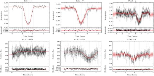
Author notes

Winton Fellow.

Juan Carlos Torres Fellow.