Hypercompact stellar clusters: morphological renditions and spectrophotometric models

ABSTRACT

Numerical relativity predicts that the coalescence of a black hole (BH) binary causes the newly formed BH to recoil, and evidence for such recoils has been found in the gravitational waves observed during the merger of stellar-mass BHs. Recoiling (super)massive BHs are expected to reside in hypercompact stellar clusters (HCSCs). Simulations of galaxy assembly predict that hundreds of HCSCs should be present in the halo of a Milky Way (MW)-type galaxy, and a fraction of those around the MW should have magnitudes within the sensitivity limit of existing surveys. However, recoiling BHs and their HCSCs are still waiting to be securely identified. With the goal of enabling searches through recent and forthcoming data bases, we improve over existing literature to produce realistic renditions of HCSCs bound to BHs with a mass of 10⁵ M_⊙. Including the effects of a population of blue stragglers, we simulate their appearance in Pan-STARRS and in forthcoming Euclid images. We also derive broad-band spectra and the corresponding multiwavelength colours, finding that the great majority of the simulated HCSCs fall on the colour–colour loci defined by stars and galaxies, with their spectra resembling those of giant K-type stars. We discuss the clusters properties, search strategies, and possible interlopers.

black hole physics, gravitational waves, galaxies: nuclei, galaxies: star clusters: general

1 INTRODUCTION

General relativity predicts that a burst of gravitational waves (GW) is emitted during the coalescence of two compact objects (e.g. Fitchett 1983; Redmount & Rees 1989; Wiseman 1992). The first direct observation of such an event took place on 2015 September 14, marking the advent of a new era. Abbott et al. (2016) inferred that the emission originated from the merger of two black holes (BHs) with masses |$29_{-4}^{+4}$| and |$36_{-4}^{+5}$| M_⊙.

Asymmetries in the merging objects (i.e. different masses and spins) are expected to produce asymmetries also in the GW emission, leading to a net flux of linear momentum. To conserve linear momentum, the merging binary and the resulting object recoil accordingly. They get a ‘kick’. The amplitude of such kick is largest for BH binaries, and it must be computed numerically. When this became possible, the expected amplitudes of order 10² km s⁻¹ were confirmed (Pretorius 2005; Baker et al. 2006; Campanelli et al. 2006; Pretorius 2006). Moreover, much larger values, as high as 5000 km s⁻¹ for special configurations, were also obtained (e.g. Campanelli et al. 2007; Tichy & Marronetti 2007; Brügmann et al. 2008; Rezzolla et al. 2008; Lousto & Zlochower 2011, 2013). Via the modelling of GW waveforms, recoil velocities have been estimated for GW170104 (Healy et al. 2018), and for GW150914 (Healy et al. 2019; Lousto & Healy 2019), where the inferred kick attains −1500 km s⁻¹.

As the escape velocities from the most massive galaxies are estimated to be below 3000 km s⁻¹ (e.g. Merritt et al. 2004), the predictions outlined above attracted a great deal of interest: merging galaxies can bring two supermassive black holes (SMBHs) together (e.g. Begelman, Blandford & Rees 1980), and the resulting SMBH could experience a recoil large enough to be appreciably displaced from the centre of the host galaxy, or even ejected in intergalactic space. The first scenario, where the BH receives a moderate kick and is not ejected from its host galaxy, is the one expected to be the most common: the recoiling BH would oscillate about the galaxy centre loosing energy via dynamical friction at each passage through the core of an early-type galaxy (e.g. Gualandris & Merritt 2008), or through the disk and bulge of a late-type galaxy (e.g. Blecha & Loeb 2008; Kornreich & Lovelace 2008); bursts of accretion would follow the passage through a gas-rich disc (e.g. Blecha & Loeb 2008). The second scenario, where recoiling velocities are high enough to remove an SMBH from its host galaxy, is much more unlikely than the first: attaining recoiling velocities in excess of a few hundreds km s⁻¹ requires special configurations for the BH binary (e.g. Lousto & Zlochower 2011; Lousto et al. 2012). For instance, gas accretion on to the merging SMBHs could align their individual spins with the binary orbital angular momentum, heavily hampering the recoil velocity, and producing kicks which are, for the most part, below 100 km s⁻¹ (e.g. Bogdanović, Reynolds & Miller 2007; Dotti et al. 2010).

Depending on the environment where it is born, the recoiling BH carries along a mixture of gas and stars, with the amount of matter bound to the recoiling BH being inversely proportional to the kick velocity, V_k. When the recoiling BH originates in a gas-rich environment (the ‘wet’ merger scenario), for example from a binary embedded in a gaseous disc, then, assuming a disc with a mass much smaller than the binary, the recoiling BH is expected to carry with it a punctured disc with outer radius |$r\propto V_{k}^{-2}$|⁠, and mass |$M_{\mathrm{disc}} \propto V_{k}^{-2.8}$|⁠. This gas will be accreted within a few million years (e.g. Bonning, Shields & Salviander 2007; Loeb 2007).

When gas is not present (the ‘dry’ merger scenario), then the recoiling SMBH will still carry with it a retinue of stars: those located within a distance |$r_{k} \equiv GM_{\bullet }/V_{k}^{2}$| from the SMBH will remain bound after the kick, and the predicted stellar mass of the cluster is M|$_{\star } \propto V_{k}^{-2(3-\gamma)}$|⁠, with γ the slope of the stellar density distribution before the kick (Komossa & Merritt 2008; Merritt, Schnittman & Komossa 2009; O’Leary & Loeb 2009). The effective radius for these clusters is predicted to depend on a number of parameters: the central velocity dispersion of the host galaxy, the stellar density distribution prior to the kick, and the dynamical status of the nucleus (collisional or collisionless, Merritt et al. 2009); while the largest clusters could extend as much as a few tens of parsecs (similarly to globular clusters and ultracompact dwarf galaxies), the great majority is predicted to have sizes below 1 pc (hence the appellative ‘hypercompact’) and velocity dispersion in excess of a few tens of km s⁻¹ (Merritt et al. 2009; O’Leary & Loeb 2009), much larger than the typical velocity dispersion of globular clusters (approximately 10 km s⁻¹, e.g. Pryor & Meylan 1993).

The observed velocity dispersion of an hypercompact stellar cluster (HCSC) is of primary importance: as simulations predict a simple proportionality with the kick velocity (σ_obs ≈ V_k/3.3, Merritt et al. 2009), it is clear that a population of HCSCs observed in the halo of a galaxy would open the door to a direct determination of the kick velocity distribution, therefore constraining the merger history of the host galaxy, the models of galaxy assembly, the simulations of merging BHs and the assumptions upon which they rest. From a determination of M_⋆ and V_k, one could also derive γ, gaining insights on the distribution of stars in the nucleus at the time of the merger.

The predicted number of HCSCs bound to the Milky Way (MW) ranges from a few tens to a few thousands: O’Leary & Loeb (2009) estimated that an MW-like galaxy which undergoes a hierarchical assembly, with no major mergers since redshift z = 1, should retain in its halo hundreds of HCSCs bound to BHs with masses in the range 10³ ≤ M_• ≤ 10⁵ M_⊙, and tens of clusters bound to BHs with M_• ≳ 10⁵ M_⊙. These HCSCs were ejected from the shallow potential well of the building blocks of the main galaxy, and they were trapped in the region which collapsed to make the MW-like galaxy. Later, Rashkov & Madau (2014) used the cosmological simulation Via Lactea II (Diemand et al. 2008) to predict the properties of a population of relic intermediate-mass BHs (IMBHs) in the halo of an MW-type galaxy. These too are leftovers of the galaxy hierarchical assembly. They identified a population of ‘naked’ IMBHs (their subhaloes were destroyed during infall) and ‘clothed’ IMBHs (residing in the nuclei of stripped galaxies). The naked BHs make up 40–50 per cent of the total population and are mostly located within 50 kpc of the halo centre, where tidal stripping is more effective. These BHs are also associated with compact stellar clusters, not necessarily bound to recoiling BHs, but simple residuals of a stripped NSC. The total number of the relic population ranges between 70 and 2000, depending on the BH seeding scenario and the steepness of the M_•–σ relation (Ferrarese & Merritt 2000; Gebhardt et al. 2000) adopted to populate the nuclei. They would be spatially resolved and with apparent magnitude as bright as m_V ≈ 16, in the scenario producing the most massive IMBHs.

Considering the challenges that an all-sky survey would imply to search for HCSCs in our own galaxy, Merritt et al. (2009) produced a prediction for nearby galaxy clusters, where the limited angular extension would ease the task: they estimated that Virgo should contain one HCSC with apparent magnitude K ≤ 20 and up to 150 with K ≤ 26.

Observational evidence for the existence of HCSCs and recoiled SMBHs is scant. O’Leary & Loeb (2012) mined the 7th data release of the Sloan Digital Sky Survey (SDSS DR7) finding 100 HCSC candidates with photometric properties consistent with theoretical models, however, to date none of these has been confirmed as a genuine HCSC. Postman et al. (2012) argued that the SMBH of the Abell 2261 brightest cluster galaxy was ejected via gravitational recoil, and they identified four HCSC candidates located in the vicinity of the galactic nucleus – possible carriers of the putative ejected SMBH; later, Burke-Spolaor et al. (2017) showed that two of them are consistent with either dwarf galaxies or stripped nuclei, while the nature of the other two remains poorly constrained. The puzzling object HVGC-1 was tentatively interpreted as a hypervelocity globular cluster ejected from the Virgo cluster in the aftermath of a three-body interaction; the HCSC scenario was dismissed because of the low metallicity and the low velocity dispersion (σ_⋆ ≤ 80 km s⁻¹, too low when compared with the putative kick velocity, V_k ≥ 1025 km s⁻¹, Caldwell et al. 2014). Boubert et al. (2019) considered the possibility that the fastest star in Gaia DR2 is bound to a recoiling IMBH, but they favoured an interpretation where the measurement is spurious. Several other sources have been proposed as candidate recoiling SMBHs (presumably clothed with an HCSC), but alternative interpretations remain often equally viable and difficult to rule out conclusively (e.g. Bonning et al. 2007; Komossa, Zhou & Lu 2008; Shields et al. 2009; Batcheldor et al. 2010; Civano et al. 2010; Robinson et al. 2010; Jonker et al. 2010; Tsalmantza et al. 2011; Eracleous et al. 2012; Koss et al. 2014; Lena et al. 2014; Menezes, Steiner & Ricci 2014; Markakis et al. 2015; Chiaberge et al. 2017; Kalfountzou, Santos Lleo & Trichas 2017; Makarov et al. 2017; López-Navas & Prieto 2018).

With the aim of facilitating the task of their identification, we present spectroscopic and photometric renditions of HCSCs bound to recoiling BHs with a mass of 10⁵ M_⊙. Photometric renditions are built upon the dynamical simulations of Merritt et al. (2009) and O’Leary & Loeb (2012). The effects of a population of blue stragglers are accounted for, in both photometry and spectroscopy. Methods and results are presented in Section 2, where we provide details on spectroscopic simulations, on the derivation of colours for a number of publicly available data sets, and on the rendition of the cluster morphology, which includes the effects of kick velocity and dynamical ageing. In Section 3, we discuss the derived properties of HCSCs, along with search strategies and challenges in their identification. We sum up and conclude in Section 4.

Through the paper, we assume the cosmological parameters H₀ = 69.6, Ω_M = 0.286, and Ω_vac = 0.714.

2 METHODS AND RESULTS

In this section, we provide details on the methods and tools used to simulate spectra, colours, and morphology of HCSCs. Results are also shown.

2.1 Synthetic spectra

We simulated a set of hypothetical HCSC spectra for clusters with about 10 000 stars – the number of stars expected for a cluster bound to a 10⁵ M_⊙ BH ejected at low velocity (v_k = 150 km s⁻¹), and relatively young (time since the kick τ_k < 10⁷ yr). For each cluster we assumed a single stellar population and a single metallicity. However, the grid of models presented here allowed to explore the effects of different metallicities and ages of the stellar population on the cluster properties.

To simulate the integrated spectra of HCSCs, we generated atmospheric models for the individual stars which make up the cluster, we derived the corresponding spectra via a spectral synthesis software, and we co-added the individual spectra to produce an integrated spectrum for the HCSC as a whole. Additional details on the steps of this process are given below.

As a starting point, we created a Hertzsprung–Russell diagram to represent every evolutionary stage present in the chosen stellar population. These diagrams were produced using the web interface cmd¹ v3.3 in conjunction with the ‘PAdova and TRieste Stellar Evolutionary Code’ (parsec v1.2S, Bressan et al. 2012; Tang et al. 2014; Chen et al. 2015); the evolutionary tracks provided us with the physical parameters for each of the stars present in the star cluster. In the cmd interface, we chose the YBC version of the bolometric correction (Chen et al. 2019), and we included the effects of circumstellar dust adopting the following composition: 60 per cent silicate plus 40 per cent aluminum oxide for M stars, and 85 per cent amorphous carbon plus 15 per cent silicon carbide for C stars (Groenewegen 2006).

To generate the isochrones we adopted a Kroupa initial mass function following a two-part power law (Kroupa 2001, 2002) and we generated a grid of models with metallicities Z = 0.0002, 0.002, 0.02 (solar), 0.03, 0.07, and ages of the stellar population τ_⋆ = 1, 7, and 13 Gyr. To extract stellar parameters we inverted the cumulative mass function generated via cmd, extracting randomly the parameters until we reached the expected total mass bound to the recoiling BH. The stellar parameters were then used to create a series of atmospheric models using atlas9 (Kurucz 1970). atlas9 is a local thermodynamic equilibrium 1D plane-parallel atmospheric modelling software which uses opacity distribution functions to reduce the computational time. These atlas9 atmospheres are used to generate synthetic spectra for each stellar evolutionary stage using synthe, a suite of programs requiring input model atmospheres, chemical abundances, and a list of atomic and molecular species (Kurucz & Furenlid 1979; Kurucz & Avrett 1981); we adopted the atomic and molecular lines lists provided in the Castelli website.² Finally, individual stellar spectra were co-added to create a synthetic integrated-light spectrum for each of the star clusters of a given age and metallicity. The synthetic spectra were created with a wavelength coverage of 3000–24 000 Å at high resolutions (R ∼ 500 000), and then degraded to the desired velocity dispersions.

Blue stragglers were also included in the stellar population of the cluster with the following approach: for each isochrone of a given age, we compiled a separate set of theoretical models with ages in the range of 10–90 per cent the age of the isochrone in question. We then randomly extracted stars with masses 1–2 times the mass of the main-sequence turn-off, with the number of blue stragglers satisfying the relation by Xin et al. (2011) for Galactic open clusters:

$$\begin{eqnarray*} N_{\mathrm{ BS}} = (0.114 \pm 0.006) N_{2} - (1.549 \pm 0.731), \end{eqnarray*}$$

(1)

where N₂ is the number of stars within two magnitudes below the main-sequence turn-off. With this approach the fraction of blue stragglers is approximately 0.3, 1, and 2 per cent in clusters with a stellar population of age τ_⋆ = 1, 7, and 13 Gyr, respectively. Here we note that this approach naturally yields a population of yellow and red stragglers, that is evolved blue stragglers which left the main sequence (e.g. Kaluzny 2003; Leiner et al. 2016).

The resulting spectra are shown in Fig. D1 for a range of metallicities and ages, along with the best-matching spectra from the Pickles (1998) atlas.

2.2 Colours

Using instrument-specific transmission curves and the synthetic spectra described in Section 2.1, we derived the expected colours, in the different filter bands, for a number of publicly available data sets, namely SDSS (the Sloan Digital Sky Survey, York et al. 2000; Blanton et al. 2017), KIDS (the Kilo-Degree Survey, de Jong et al. 2013a, b), VIKING (the VISTA Kilo-degree Infrared Galaxy Survey, Edge et al. 2013), CFHTLS (the Canada-France-Hawaii Telescope Legacy Survey, MEGACAM, Hudelot et al. 2012), Pan-STARRS (the Panoramic Survey Telescope and Rapid Response System, Chambers et al. 2016), Gaia (the Global Astrometric Interferometer for Astrophysics, Perryman et al. 2001; Gaia Collaboration 2016), NGVS (the Next Generation Virgo Cluster Survey, Ferrarese et al. 2012), and 2MASS (the Two Micron All-Sky Survey, Skrutskie et al. 2006). Results are presented in Fig. 1, where colours are shown for different stellar ages and metallicities, and compared with the observed colours of stars, galaxies, and globular clusters.

Figure 1.

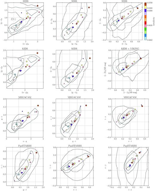
Colour–colour plots for different instruments and different bands. Circles: expected colours for the HCSCs with metallicity as indicated in the colour bar, and with circle size proportional to the age of the stellar population (1, 7, or 13 Gyr); dashed black contours: randomly selected galaxies; and solid grey contours: randomly selected stars. Contour labels indicate the fraction of data outside the contour. Gaia: black dashed contours are quasi stellar objects (QSOs). NGVS: orange crosses are Galactic halo stars and blue diamonds are M31 globular clusters, the green triangle is the hypervelocity cluster HVGC-1 (data from Caldwell et al. 2014); galaxies, which would be located above the globular clusters, have been omitted from this plot. 2MASS: solid contours are point sources; and dashed contours are extended sources. Details on the origin and selection of the plotted data are given in Appendix  B (continues on next page).

Transmission curves were taken from the Spanish Virtual Observatory Filter Profile Service.³ Best-fitting curves to the predicted colour–colour loci are given in Appendix  A.

2.3 Morphology

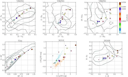
We used skymaker (Bertin 2009) to produce mock images of HCSCs corresponding to observations conducted with Pan-STARRS (Chambers et al. 2016) and with the Near Infrared Spectrometer and Photometer (NISP) on board the forthcoming Euclid telescope (Laureijs et al. 2011). The result is shown in Fig. 2.

Figure 2.

Renderings of HCSCs for Pan-STARRS (first and second columns) and for Euclid/NISP (third and fourth columns). The cluster is bound to a 10⁵ M_⊙ BH at distances of 10 and 30 kpc from the observer, as indicated in the bottom left corner of each panel. The kick velocity increases from 150 to 500 km s⁻¹ as indicated in the top left corner of the panels. Simulated exposure times are t = 40 s for Pan-STARRS and t = 116 s for NISP. The age of the stellar population is τ_* = 7 Gyr, and the metallicity is Z = 0.02 (solar). The time since the kick is τ_k = 100 in N-body units, or τ_k = 1.25, 0.27, 0.03 × 10⁴ yr; we note, however, that this dynamical state of the cluster should persist for a relaxation time (10⁶–10⁷ yr). The number of stars in each cluster is approximately 10 000, 3000, and 500 (decreasing at higher values of V_k). The renderings correspond to the projection on the xy plane of Fig. D2, where the kick-induced asymmetry is maximized. Flux units: counts. Note the spatial-scale change in each row. Arbitrary contours are added to highlight the clusters morphology.

skymaker is a simulator of astronomical images; it takes as input a parameter file and a catalogue. The former specifies a number of parameters, such as seeing, pixel scale, telescope details, and central wavelength, among many others. The latter is a catalogue of coordinates, magnitudes, and a code to discern between stars and galaxies. If a point spread function (PSF) is not provided, then the software derives one taking into account blurring due to the atmosphere, to the telescope motion, diffraction and aberration features, effects due to optical diffusion (i.e. scattered light), and intra-pixel response (i.e. the sensitivity variation within a pixel). Once the objects in the catalogue are rendered, a sky background is added along with Poissonian and Gaussian noise, representing photon noise and noise due to electronics, respectively.

To create the input catalogue for skymaker, we adopted the stellar positions derived via N-body simulations by Merritt et al. (2009), Fig. D2. The simulation was realized with N = 1.5 × 10⁴ equal-mass particles and assuming an initial power-law density profile ρ ∝ r^−7/4. An instantaneous kick of magnitude V_k was delivered to the cluster along the −X-direction at t = 0. We used the results obtained at t = 100 (physical units can be obtained by multiplying the N-body time by GM_•/V|$_{k}^3$|⁠, with G the gravitational constant, M_• the BH mass, and V_k the kick velocity). Stellar locations were derived by inverting the cumulative mass profile derived from the N-body simulation. The process consisted of four steps: (1) we selected a random number uniformly distributed between zero and the total mass of the cluster; (2) by inverting the cumulative mass profile we selected a radial distance from the cluster centre; (3) we picked the N-body point located at that radial distance; and (4) the star coordinate was extracted from a Gaussian distribution centred at the location of the N-body point, and characterized by a standard deviation given by 10 per cent the value of its 3D distance from the cluster centre.

The number of stars in the cluster, right after the kick, was determined so that the bound stellar mass would amount to:

$$\begin{eqnarray*} M_{b} = 11.6\gamma ^{-1.75} \times M_{\bullet } \left(\frac{GM_{\bullet }}{r_{\bullet }V_{k}^2}\right)^{3-\gamma }, \end{eqnarray*}$$

(2)

where γ, here assumed to be 7/4, as in the N-body simulation, is the slope of the stellar density profile before the kick (ρ ∝ r^−γ), and r_• is the radius containing an integrated mass in stars equal to twice M_•. Equation (2) was derived by combining equations (5), (7), and (8) in Merritt et al. (2009). The scaling relation adopted for r_• is:

$$\begin{eqnarray*} r_{\bullet } \approx 8\ \mathrm{pc} \left(\frac{M_{\bullet }}{10^7M_{\odot }}\right)^{0.46}, \end{eqnarray*}$$

(3)

which we derived by fitting the data presented by Merritt et al. (2009) in their fig. 12 for ‘power-law’ galaxies, that is galaxies with a deprojected inner density profile steeper than R^−0.5 (e.g. Lauer et al. 1995, but see also Graham 2013). Although ‘core’ galaxies (those with a central density profile shallower than R^−0.5), are more likely to result from a history of mergers (e.g. Ebisuzaki, Makino & Okumura 1991; Makino & Ebisuzaki 1996; Merritt 2006), and therefore more likely to be the progenitors of HCSCs, we prefer to use the scaling relation derived for ‘power-law’ galaxies as it is better constrained at the low-mass end of the SMBH mass distribution, which is the focus of this work. The difference between the extrapolated values of r_• is, however, small: for M_• = 10⁵ M_⊙, we get r_{•, core} ≈ 0.8 r_{•, power-law}; furthermore, if one would extend fig. 12 of Merritt et al. (2009) to lower masses, such difference would turn out to be much smaller than the scatter in the data points.

To derive magnitudes, we inverted the evolved integrated initial mass functions produced via parsec along with the isochrones (Section 2.1). Stellar masses and the corresponding magnitudes were then extracted and randomly assigned to the N-body points. In this process, we ignored the effects of mass segregation as O’Leary & Loeb (2012) found only moderate evidence that this process was taking place in their models, even though the dynamical simulations included stars spanning a factor 10 in mass. Similar results on mass segregation were obtained for simulations of globular clusters with a nuclear BH: the BH quenches mass segregation by scattering sinking particles out of the core (e.g. Baumgardt, Makino & Ebisuzaki 2004; Gill et al. 2008).

We assumed the telescope and seeing parameters indicated in Appendix  C, a distance to the cluster of 10 and 30 kpc, and a BH mass of 10⁵ M_⊙. Finally, we point out that an accurate representation of the cluster morphology should take into account the cluster expansion. Dynamical studies conclude that the radius enclosing a fixed number of stars evolves as r ∝ t^2/3, however the evolution is expected to deviate from this law when the number of stars in the cluster becomes small (e.g. O’Leary & Loeb 2012, and references therein). Furthermore, Merritt et al. (2009) warn that the true evolution of the cluster is likely affected by a number of phenomena which are still poorly understood and not fully implemented in dynamical simulations. For these reasons, as Merritt et al. (2009), we ignored the cluster expansion.

2.3.1 Effect of different kick velocities

As equation (2) shows, the stellar mass bound to the recoiling BH right after the kick is a function of the kick velocity. The effects of different kick velocities on a HCSC bound to a 10⁵ M_⊙ BH are shown in Fig. 2, which simulates a 40 s Pan-STARRS-DR1 exposure in the r band, and a 116 s Euclid/NISP exposure in the J band (these are the nominal durations of single exposures for the 3π Pan-STARRS survey, e.g. Schlafly et al. 2012, and for the wide-field survey planned for Euclid, e.g. Carry 2018).

2.3.2 Cluster evolution after the kick

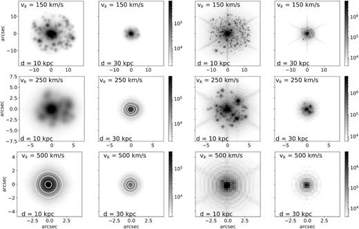
After receiving the GW kick, the cluster is believed to evolve via resonant relaxation (Merritt et al. 2009; O’Leary & Loeb 2012). More specifically, a fraction of the stars is lost via tidal disruption events, and a fraction is ejected because of large-angle scattering (Henon 1969; Lin & Tremaine 1980). Merritt et al. (2009) and O’Leary & Loeb (2012) performed dynamical simulations to quantify the effects due to these processes, finding that the rate of stellar loss depends on the mass of the BH, with clusters around more massive BHs evolving more slowly than clusters around lower mass BHs.

To implement the time evolution, we used the results of the Fokker–Planck simulation of O’Leary & Loeb (2012) for a cluster bound to a 10⁵ M_⊙ BH. We reproduced their function using a smoothly broken power law:

$$\begin{eqnarray*} f(t) = A\left(\frac{t}{t_{b}}\right)^{-\alpha _1}\left\lbrace \frac{1}{2}\left[1 + \left(\frac{t}{t_{b}}\right)^{1/\Delta }\right]\right\rbrace ^{(\alpha _1 - \alpha _2)\Delta }, \end{eqnarray*}$$

(4)

where the amplitude A was matched to the number of stars bound to the BH at the time of the kick (τ_k ≤ 10⁶ yr), and the remaining parameters being t_b = 6.79 × 10⁶ yr, α₁ = −0.12, α₂ = 0.34, and Δ = 1.76. The resulting images, derived from the xy panel of Fig. D2, are presented in Figs 3(a) and (b), for Pan-STARRS and Euclid/NISP, respectively.

Figure 3.

(a) Mock Pan-STARRS-DR1 images of an HCSC as a function of the time since the kick, τ_k, and as a function of the age of the stellar population, τ_⋆. Assumed parameters are: kick velocity V_k = 150 km s⁻¹, distance = 10 kpc, BH mass M_• = 10⁵ M_⊙. The number of stars in each panel (left to right) is approximately 8000, 5000, 2000, and 1000. (b) As in Fig. 3(a) for Euclid/NISP.

3 DISCUSSION

To narrow down the number of HCSC candidates from the mare magnum of galaxies and stars sampled in a survey, one can start with a selection based on colour. For unresolved candidates, this might be the only parameter available, followed by an estimate of the absolute magnitude, kinematics, and by the stellar velocity dispersion, if spectroscopy is feasible. Resolved candidates will offer the possibility of further cuts based on the morphology. We discuss these aspects in the following sections.

3.1 Colours

Fig. 1 shows that the predicted optical and NIR colours of the clusters are not peculiar with respect to the general population of stars and galaxies. This is not surprising, as we have not implemented (and we are not aware of) any peculiar process which could be at play in these clusters, and which could leave a distinctive imprint on their stellar population.

In the optical, the predicted colours follow the locus of stars and galaxies. It is only in the JHK_s colour diagram that HCSCs show an offset from the peaks of the distributions for stars and galaxies. It is for this reason that adding an NIR colour-cut to a set of candidates selected on the basis of their optical colours decreases the sample size by a factor ten. Still, the number of candidates obtained via a search based solely on optical and NIR colours is too large to be constraining.

Muñoz et al. (2014) showed that a uiK_s colour–colour diagram allows for a clean separation between stars, globular clusters, and galaxies. Such colour–colour diagram was used by Caldwell et al. (2014) to investigate the nature of the hypervelocity cluster HVGC-1, finding that it falls in the region defined by the globular clusters. We computed the expected uiK_s colours for our sample of simulated HCSCs (Fig. 1, central panel, bottom row); unfortunately, we found a large scatter which hampers the diagnostic power of this diagram in the search for HCSCs.

It is clear that a colour selection alone will not yield a suitable sample of candidates, unless it turns out that some peculiar process takes place into the exotic environment of such clusters, leaving a strong signature on its spectrophotometric properties, for example an enhanced rate of stellar mergers leading to an excess of blue stragglers. Preliminary simulations show that increasing the number of blue stragglers affects mostly the ultraviolet (UV) colours of subsolar metallicity clusters; instead, adopting the GALEX (Bianchi & GALEX Team 1999) transmission curves, HCSCs with metallicity Z ≥ 0.02 (solar and above) have always colours in the range 6 ≤ (FUV − NUV) ≤ 8, independently of the presence of blue stragglers. Evolved stragglers falling on the red giant branch (RGB) affect optical and NIR colours introducing a higher variance in the result of the simulation (e.g. making a young cluster with solar metallicity appear similar to a supersolar metallicity cluster with an old stellar population).

We draw the reader’s attention to the following three points. First, subsolar metallicity clusters might be unusual: HCSCs, being dislodged galactic nuclei, will likely show supersolar metallicity, and, being residuals of the galaxy-assembly process, their stellar population might also be old (e.g. if an HCSC was ejected at redshift z = 1, and no star formation took place in it, then its stellar population should be at least 7 Gyr old). While an old stellar population with supersolar metallicity might seem an odd combination, we note that several times supersolar solar metallicity has been inferred for the broad-line regions of high-redshift quasars, for example Juarez et al. (2009). The second point to note is that, to date, the only instrument performing sky surveys and sensitive in the near UV is Gaia (the G_BP passband covers the wavelength range 330–680 nm, e.g. Maíz Apellániz & Weiler 2018; Weiler 2018), with no dedicated facilities planned for the foreseeable future. Unfortunately, also our predicted Gaia colours mostly follow the stellar locus. Finally, a pilot search through public data bases shows that only a tiny fraction (below 1 per cent) of candidate HCSCs with optical and infrared (IR) coverage posses also good quality UV data.

We note that our models assume a single stellar population (including blue stragglers) and a single metallicity. On the other hand, HCSCs might share some properties with ancient nuclear star clusters (NSCs): if an NSC was present at the time of the recoil, the HCSC would consist of a subset of stars from the inner region of the NSC. The study of these compact objects is still in its infancy, and it is limited to the local Universe, however, it is becoming clear that they are characterized by complex stellar populations (e.g. Mastrobuono-Battisti et al. 2019; Neumayer, Seth & Boeker 2020). While our individual models for HCSCs might be simplistic, the overall set explores a range of ages and metallicities, including some extreme cases. Clusters with more complex star formation histories fall within the colour–colour loci defined by the simple models presented here, with the scatter in the distribution being inversely proportional to the number of stars bound to the BH. By comparison, Merritt et al. (2009) assumed a single stellar population and a metallicity following a Gaussian distribution; O’Leary & Loeb (2012) proposed two models, the first with constant star formation rate for the 5 Gyr preceding the GW-kick, the second with a single stellar population formed at the time of the kick; furthermore, they explored three metallicity histories: a constant solar metallicity, a constant subsolar metallicity (Z = 2 × 10⁻⁴), and the estimated time evolution for the Galactic Centre. The ugr colours derived here for SDSS can be directly compared with those derived by O’Leary & Loeb (2012). The models produce consistent results, with the larger scatter recovered here in the red side of the colour diagram being ascribed to bright evolved blue stragglers.

To summarize, the combination of parameters producing models which deviate from the bulk of the population of stars and galaxies corresponds to supersolar metallicities and old stellar ages. In light of the observations of supersolar metallicities in the nuclei of high-redshift quasars, this combination, although unusual, might not be unrealistic, allowing to select ancient HCSCs.

In the following section, we show that an HCSC with an old stellar population resembles K and M giant stars, and we highlight the spectrophotometric differences between the two classes of objects.

3.2 Spectra

In Fig. D1, we presented the model spectra derived as explained in Section 2.1. Our derivation of the spectra did not take into account the internal dynamics of the cluster and the resulting shape of the absorption line profiles; for this we refer the reader to Merritt et al. (2009), where the authors dealt with this aspect in great detail. Rather, we will compare the model spectra with the observed spectra of single stars to identify the most probable interlopers, and to identify any difference – besides a high velocity dispersion (i.e. strongly broadened absorption lines) – that would allow to distinguish stars from clusters.

We compared the models with the stellar spectra of the Pickles (1998) atlas, a library of 131 stellar spectra at solar abundance, including all normal spectral types and luminosity classes. We matched the binning of our models and the Pickles spectra, and we selected those resembling the most to the HCSC models (i.e. those producing a smaller residual when subtracted from the model). In Table 1 we indicate, for each metallicity and stellar population age assumed for the cluster, the best-matching spectrum (multiple spectra are indicated whenever the residuals differ by less than 10 per cent). In Fig. D1, we show the simulated spectra, the best-matching spectra from the Pickles atlas, and the residuals.

Table 1.

Spectral type of single-star spectra from the Pickles atlas library resembling the most an HCSC simulated with the metallicity and stellar population age indicated in the table. Spectral class indicated in upper case letter, luminosity class indicated with roman lower case letters. The prefixes r and w indicate metal-rich and metal-weak stars, respectively.

Metallicity	Stellar population age (Gyr)
	1	7	13
0.0002	G0 iii	K0 v	G8 v, K0 v, G0 iii
0.002	F02 iv, F0 v	rK5 iii	rK2 iii
0.02	M2 iii, M1 iii	(w)K0 iii	wK0 iii, K2 v
0.03	F8 iv, G0 iv	M1 iii, M0 iii	wK4 iii
0.07	(w)K3 iii	K2 iii	M2 iii, M3 iii

From Table 1, we can see that HCSCs with a young stellar population (τ_⋆ ≈ 1 Gyr) and subsolar metallicity resemble G and F stars, either on the main sequence, or on the giant and subgiant phases. At the other end of the spectrum, clusters with an old stellar population (τ_⋆ ≈ 13 Gyr) and supersolar metallicity resemble giant K and M stars. Overall, most of the times, the simulated spectra resemble those of giant K stars. It is, therefore, likely that a colour–colour selection alone would be heavily contaminated by such objects.

How could we distinguish an unresolved HCSC from a giant star? Any distance information would help constraining the absolute magnitude of the candidates, applying a further selection cut on the sample. Moreover, the plots presented in Fig. D1 show often, but not systematically, a blue excess in the spectra of HCSCs. This is likely due to the contribution of the hottest main-sequence stars and the blue stragglers in the cluster.

We note, again, that the addition of a population of blue/yellow/red stragglers acts as a confounding ingredient, adding stochasticity to the appearance of the cluster: simulations which do not include stragglers produce spectra which age as expected, that is with the peak shifting towards longer wavelengths and emission in the red portion of the spectrum becoming more and more prominent as the age of the stellar population increases. The addition of stragglers, instead, does not simply contribute with a population of blue stragglers, adding emission to the blue spectral component. Rather, this population also contributes with a few bright giant stars giving a major contribution to the integrated spectrum, ageing, instead of rejuvenating, the appearance of the cluster. We also note that the adopted number of blue stragglers (0.3, 1, and 2 per cent for τ_⋆ = 1, 7, and 13 Gyr) could be a lower limit: as explained in Section 2.1, this fraction was derived for Galactic open clusters, where the stellar density is much lower than the one expected for HCSCs. The high density in the nuclei of HCSCs might enhance the production rate of blue stragglers.

To summarize, the simulated spectra of HCSCs often resemble those of K-type giant stars, however, the presence of a blue excess could be used to distinguish an unresolved HCSC from a single star.

3.3 Morphology of a resolved HCSC

Figs 2, and 3(a) and (b) show rendered versions of the N-body model presented in Fig. D2. For this model, the time since the kick is t = 100 × GM_•/V|$^{3}_{k}$|⁠; although this quantity amounts to 2700 yr for M_• = 10⁵ M_⊙ and V_k = 250 km s⁻¹, this state of the cluster should be representative for a full relaxation time, that is approximately 10⁶ yr. After that time, we assume that the cluster starts loosing stars as described in Section 2.3.2.

Fig. 2 shows the effect of increasing kick velocities for a cluster with solar metallicity (Z = 0.02), a stellar population of intermediate age (τ_* = 7 Gyr), and located at distances of 10 and 30 kpc. The first two columns show the rendering of a Pan-STARRS r-band image. At the resolution of Pan-STARRS (median seeing θ_r ≈ 1.2 arcsec and pixel size p = 0.25 arcsec), the cluster corresponding to V_k = 150 and 250 km s⁻¹ is (barely) resolved to a distance of 30 kpc, showing evidence for a low-density envelope and a denser, compact core. For V_k = 500 km s⁻¹ the cluster is featureless, at visual inspection, and barely resolved at best. With the adopted saturation level and exposure time (reflecting the duration of a single exposure in the 3π Pan-STARRS survey, Schlafly et al. 2012), the core is saturated when V_k = 150 km s⁻¹ and for V_k = 250 km s⁻¹ at d = 10 kpc.

The last two columns of Fig. 2 show the rendering of a Euclid/NISP J-band image. As NISP will be diffraction-limited, with a pixel size of p ≈ 0.3 arcsec, it is not surprising to find a much sharper image, with the cluster being resolved also for V_k = 500 km s⁻¹ at d = 10 kpc. The core is saturated in all six renderings. It must be stressed, however, that the rendering depends on the background and the instrument PSF, two parameters which, at the time of writing, are not well known.

An observable quantity that one could derive for an HCSC and use it to mine catalogues, similarly to O’Leary & Loeb (2012), is the Petrosian radius, that is the radius where the local surface brightness equals the average surface brightness within that radius (Petrosian 1976). However, this parameter is not ideal for clusters which are resolved and which include bright stars in their halo. Such clusters will be treated as a collection of individual objects in a survey catalogue. Moreover, for the cluster as a whole, the condition defining the Petrosian radius might be satisfied at multiple radii because the local surface brightness would not be monotonic. Therefore, this parameter can not be used for most of the scenarios explored here.

3.3.1 Kick signatures

From Fig. D2, it is clear that at t = 100 the cluster core is still flattened, with the major axis aligned with the kick direction. However, this important morphological feature (it carries information on the kick direction) is lost in the rendered images presented in Figs 2, and 3(a) and (b). The reason resides in the combination of stellar density profile and resolution effects: first, the cluster is characterized by a steep density profile; that is already at r ≲ 1 × GM_•/V|$^{2}_{k}$| (in N-body units), or r ≲ 0.02 pc (for M_• = 10⁵ M⊙ and V_k = 150 km s⁻¹), the stellar density is 10²–10⁵ times lower than it is at the very nucleus (the exact value depends on the adopted density distribution before the kick, see fig. 3 in Merritt et al. (2009); we used simulations produced from an initial density ρ ∝ r^−7/4). Second, when magnitudes and stellar evolutionary stages are assigned to the N-body points, a few of them correspond to the evolutionary stages ‘RGB’, ‘core helium burning’, or ‘EAGB’. These are all bright stars (−5 < M_J < 3, −1 < M_r < 3), and the great majority of them are packed in the central density cusp. As a result, such bright stars are not resolved in the mock observations, and the convolution with the PSF erases the photometric asymmetry which, naively, would be expected from the spatial distribution alone.

To constraint the kick direction one could, therefore, rely on the asymmetry of the extended envelope, which evaporates as time goes by. As it is evident in Fig. D2, at t = 100 GM_•/V|$^{3}_{k}$| (or after one relaxation time) stars are still distributed asymmetrically in the envelope: defining the envelope as the region outside the elliptical bulge with semimajor axes 13 and 10 (in N-body units), about 40 per cent of the envelope stars are located within the quadrant defined by position angles in the range −45: 45 deg, where PA = 0 deg corresponds to the positive side of the X-axis, or the counter-kick direction. However, Figs 3(a) and (b), which are renderings of the xy panel of Fig. D2, show that already at t ≥ 10⁷ yr such asymmetry looses its prominence. Projection effects, and higher recoil velocities (implying a lower number of bound stars), would only weaken the asymmetry and the conspicuity of the halo as a whole.

3.3.2 Light profile

What is the light profile that one would recover from an image of a resolved HCSC? Similarly to O’Leary & Loeb (2012), we derived, for the clusters rendered in Figs 3(a) and (b), the logarithmic slope of the cumulative light profile: Γ_i = d ln(I_i)/d ln(r) ≈ ln(I_{i + 1}/I_i)/ln(r_{i + 1}/r_i) and the average intensity within annuli of radius r_i = 0.23, 0.68, 1.03, 1.76, 3.00, 4.63, 7.43, 11.42, 18.20, and 28.20 arcsec (the same adopted to produce the SDSS and Pan-STARRS catalogues). The width of the annuli is δ = 1.25r_i − 0.8r_i. The derived slopes are given in Table 2; plots of the intensity profiles are shown in Fig. 4.

Figure 4.

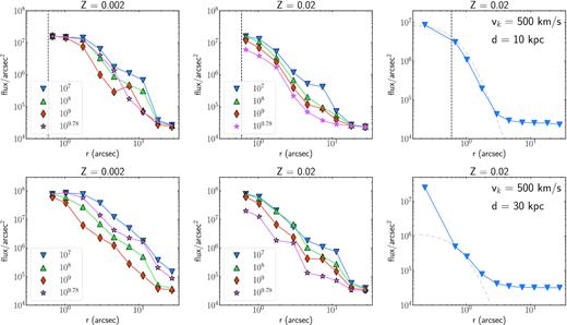
Light profiles derived from the rendered HCSCs presented in Figs 3(a) and (b) (first and second columns) and for two clusters from Fig. 2 (third column) for Pan-STARRS (top row) and Euclid/NISP (bottom row). The plot shows the average intensity of light within annuli. The adopted metallicity is indicated on top of the panels. The time since the kick (τ_k) is indicated in the legend in years for the clusters from Figs 3(a) and (b). Symbols with a solid black edge indicate the presence of saturated pixels in the nucleus. The vertical dashed line, in the top row, marks the typical FWHM/2 of the Pan-STARRS seeing in the r band. The luminosity of the older cluster with metallicity Z = 0.002 increases because of a few stars on the EAGB. For comparison, a Plummer (1911) profile, representative of globular clusters, is plotted as a dashed grey curve in the third column. We stress that the inner flattening visible in the first and second columns is due to the presence of saturated pixels.

Table 2.

Logarithmic slope of the cumulative surface brightness associated with the profiles presented in Fig. 4. Assuming M_• = 10⁵ M_⊙, V_k = 150 km s⁻¹, and d = 10 kpc, unless otherwise specified. The range of values was derived from projections of the clusters on the xy, xz and yz planes.

τk	τ⋆	Γ1	Γ2	Γ3	Γ4	Γ5	Γ6	Γ7
(Gyr)	(Gyr)
Pan-STARRS
	Z = 0.002
0.01	1	–	1.3	0.67	0.43–0.45	0.26–0.28	0.11	0.07
0.1	1.1	–	1.3	0.67	0.36–0.4	0.2–0.22	0.08–0.09	0.05
1	2	–	1.3	0.6–0.61	0.25–0.28	0.13–0.14	0.05	0.03
6	7	–	1.3	0.67	0.35–0.36	0.19–0.23	0.07–0.08	0.03–0.04
	Z = 0.02
0.01	7	–	1.3	0.55–0.56	0.21–0.22	0.12	0.05–0.06	0.03
0.1	7.1	–	1.3	0.46–0.47	0.18	0.09–0.1	0.04	0.02
1	8	–	1.1–1.2	0.38–0.39	0.14–0.15	0.08	0.03	0.02
6	13	–	0.97–1.13	0.31–0.44	0.11–0.17	0.06–0.09	0.02–0.03	0.01–0.02
	Z = 0.02, Vk = 500 km s−1
0.001	7	0.93	0.89–0.9	0.25–0.26	0.09	0.05	0.02	0.01
Euclid/NISP
	Z = 0.002
0.01	1	–	1.04	0.57	0.38	0.24–0.25	0.1–0.11	0.06
0.1	1.1	–	0.98–0.99	0.38	0.18	0.1–0.11	0.04	0.02
1	2	–	0.87–0.89	0.25–0.29	0.09–0.11	0.06	0.02–0.03	0.01
6	7	–	1.04	0.55	0.25–0.27	0.15	0.06–0.07	0.04
	Z = 0.02
0.01	7	–	1.01–1.03	0.36–0.4	0.15–0.16	0.08–0.09	0.03–0.04	0.02
0.1	7.1	–	0.97–1.03	0.34–0.38	0.16–0.17	0.09	0.03	0.02
1	8	–	0.81–0.91	0.27–0.29	0.1–0.11	0.06	0.02	0.01
6	13	–	0.62–0.67	0.18–0.21	0.07–0.08	0.04	0.02	0.01
	Z = 0.02, d = 30 kpc, Vk = 500 km s−1
0.001	7	0.18	0.18	0.05	0.02	0.01	–	–

The clusters presented in Figs 3(a) and (b) are nearby and ejected with low velocity. Therefore, they are well-resolved and individual stars in the halo can be discerned. However, Fig. 2 shows that clusters ejected at higher velocities and located further away would be almost featureless and with a smooth profile. In Fig. 4, we show the light profiles for two of those clusters, making a comparison with a Plummer (1911) profile, which is typical for globular clusters. The comparison shows that the profile of an HCSC observed with a resolution of about 1 arcsec (as for PanSTARRS and other ground-based surveys) is similar to a Plummer profile. From the light profile alone, the HCSC can, therefore, be misclassified as a globular cluster. On the contrary, observations at higher resolution (such as those expected for Euclid) reveal the presence of a nuclear cusp, which deviates from the Plummer profile.

In the barely-resolved scenario, a first step towards a better understanding of the object nature might be the inspection of the residuals obtained after fitting and subtracting a PSF. We used galfit (Peng et al. 2002, 2010) to apply this approach on the rendered Pan-STARRS images for a cluster ejected with V_k = 500 km s⁻¹ and located at d = 10 kpc (bottom left panel in Fig. 2, the adopted PSF was a star rendered with skymaker, using the same parameters adopted to render the cluster). The result is shown in Fig. 5: the residuals show clear deviations from a pure point source, suggesting a more complex nature of the object. The resolved structure is due to the presence of an extended envelope, which might be the host of one or more RGB stars. Although a small fraction of the stars in the cluster are in such evolutionary phase (i.e. <1 per cent), because of their absolute magnitude, which can be as low as M_r = −1 (M_J = −5), they have a considerable weight in determining the appearance of the cluster, both in the well-resolved scenario (where the cluster appears as an unresolved nucleus embedded into an extended envelope), and in the barely-resolved case (where a single off-centre star might be responsible for an elongated extension, resembling a slightly resolved binary star or a compact galaxy and a foreground bright star).

Figure 5.

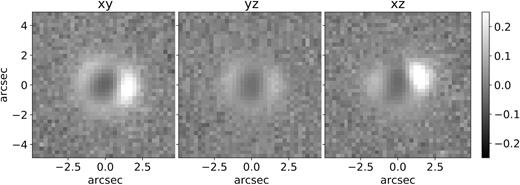
Fractional residuals obtained after fitting and subtracting a PSF from the HCSC simulated for Pan-STARRS assuming V_k = 500 km s⁻¹ and d =10 kpc.

The presence of the extended envelope depends from (at least) three factors: the age of the cluster, the kick velocity, and the metallicity. Ageing of a cluster is due to the combined action of dynamical ageing and ageing of the stellar population. Dynamical ageing is more important for low-mass clusters; for example O’Leary & Loeb (2012) found that clusters bound to BHs with mass M_• ≥ 10⁷ M_⊙ lose a very small fraction of their mass over 10¹⁰ yr, instead, the number of stars bound to a 10⁴ M_⊙ BH decreases dramatically with time. An HCSC bound to a 10⁵ M_⊙ BH is predicted to loose almost 90 per cent of its initial stars, however, also for V_k = 250 km s⁻¹, the HCSC should retain almost 3000 stars at the time of the kick, which translates into a cluster consisting of about 300 stars after 10¹⁰ yr. The effect of the stellar population ageing is clear, instead, in Figs 3(a) and (b), where, in general, the cluster envelope fades away while stars grow old; however, depending on the initial age of the stellar population, the cluster might brighten up (e.g. because of stars going through the giant phase). The kick velocity, V_k, has perhaps the most important effect on the presenze of an envelope, as shown in Fig. 2, with its size being dramatically reduced for V_k > 250 km s⁻¹. Finally, metallicity plays a mild role, with the number of bright stars decreasing at higher metallicity (high-metallicity stars loose more mass via stellar winds, e.g. Trani, Mapelli & Bressan 2014).

3.4 Search strategies and challenges

Searching for a subset of objects in a large data set requires the capability to remove false positives, and to identify the desired targets with the minimum amount of follow up observations.

The most distinctive characteristic of HCSCs is their high velocity dispersion in conjunction with their moderate absolute magnitude; this combination of parameters separates them well from the population of globular clusters, ultracompact dwarf galaxies, and elliptical galaxies (Merritt et al. 2009). However, the spectroscopic information needed to populate such a diagram is not readily available for a large data set, and it is expensive to acquire. More realistically, a search for HCSCs would start with the mining of large public data bases, with the aim of narrowing down the sample, and collect, in progressive steps and for a small subset of prime candidates, the necessary information to constrain their nature.

As shown in Sections 2.2 and 3.1, in a colour–colour diagram HCSCs fall near or at the maximum of the distribution of stars and galaxies. Therefore, a selection based on optical colours alone will be heavily contaminated by false positives, and will not produce a sample of candidates small enough to allow the collection of additional data without investing substantial effort. It is clear, however, that a data base search would greatly benefit from a multiwavelength approach: probing a larger portion of the candidate’s spectral energy distribution would set more stringent constraints. For example, our experiments show that combining optical and NIR constraints allows to reduce the sample size by a factor 10 with respect to the selection based on optical colours alone. Alternatively, one could opt for a search of old high-metallicity clusters which, in colour–colour diagrams, lie outside the region containing the bulk of the population of stars and galaxies.

When the candidates are not resolved, then kinematic and parallax information, in conjunction with absolute magnitude estimates will help constraining the nature of the candidates and remove a number of false positives: for example in a search targeting HCSCs in the Galaxy halo one could remove sources showing no evidence for proper motion, these are likely extragalactic sources; moreover, the proper motion of HCSCs should be peculiar with respect to the proper motion of other objects in the vicinity. When searching for unresolved clusters, many interlopers will be K-type giant stars, followed by G and M giants. Given a low-resolution broad-band spectrum, accurately flux-calibrated, then a blue excess in the spectrum of the candidates, at λ < 5000 Å, might help distinguishing between single stars and composite objects.

For candidates which are barely resolved, then binary stars (either visual or physical) will be an important population of interlopers. In that case, a shift in the photometric centroid from single-epoch observations at multiple wavelengths, and a periodic astrometric shift would allow to remove false positives. However, the orbital period of resolved binaries can be very long, precluding the detection of periodic astrometric shifts.

When the candidates are resolved, additional constraints can be placed on the light profile and, if bright off-centre stars are present, then Gaia might also detect the relative motion of the stars and allow to set dynamical constraints.

4 SUMMARY AND CONCLUSIONS

The possibility that hundreds of HCSCs populate galactic haloes is alluring. Their discovery would show that supermassive BHs do merge, and that GW BHs from their birthplaces (i.e. galactic nuclei). Their characterization (i.e. measurement of velocity dispersion, stellar mass, and effective radius) would allow to determine the distribution of GW recoils, would cast light on the assembly of the host galaxy, and on the distribution of stars in the nuclear environment at the time of merger. While several candidate HCSCs have been reported, none has been securely identified. If predictions are correct, they have already been imaged in existing surveys. Identifying them is, however, non-trivial. In an effort to further our understanding of these objects and to ease the task of their identification, we expanded on the existing literature by producing broad-band spectra and photometric renditions of hypothetical HCSCs bound to recoiling BHs of mass 10⁵ M_⊙. We used the renditions to derive light profiles, and the broad-band spectra to compute the colours that HCSCs would display in a number of recent data bases.

Photometric renditions were based on the dynamical simulations presented in Merritt et al. (2009) and O’Leary & Loeb (2012), which we used to implement the spatial distribution of stars and the cluster evaporation. We produced images of the clusters as they would appear in the 3π Pan-STARRS survey and in the wide-field survey of the instrument NISP on board the forthcoming Euclid space telescope. Images and light profiles were derived for a range of kick velocities, distances, metallicities, dynamical ages, and ages of the stellar population, with the inclusion of blue, yellow, and red stragglers. While clusters ejected at moderate velocities (250 km s⁻¹) and located at a distance of a few tens of kpc are barely resolved by current surveys, they can be resolved by Euclid, with both the instruments NISP and VIS (the Visible Imager, an instrument with a better resolution than NISP). When observed at a resolution of about 1 arcsec, typical of ground-based surveys, HCSCs located a few tens of kpc away and ejected with velocities above 250 km s⁻¹ would appear featureless and with light profiles resembling those of globular clusters. The inner cusp of HCSCs can be revealed, instead, with subarcsecond resolutions, such as those achievable with Euclid. The capability to resolve the light profile is important when implementing a search, as it allows to place additional constraints on the candidates (colours, we showed, have limited constraining power). It is, therefore, desirable to develop a library of models exploring the full parameter space of BH masses, stellar masses, and cluster age.

We used stellar evolutionary models to generate a set of broad-band synthetic spectra and the corresponding colours that HCSCs would display. While optical colours were previously derived by Merritt et al. (2009) and O’Leary & Loeb (2012), we computed colours for additional bands, and for specific surveys, including recent ones, such as Gaia and NGVS, among others. We covered, therefore, a larger portion of the spectrum, providing more stringent constraints for the selection of a sample. We show that most of the times, in a colour–colour diagram, HCSCs fall very close to the peak of the distribution of stars and galaxies. The exception are high-metallicity clusters (Z = 0.07) with an old stellar population (τ_⋆ = 13 Gyr). While this combination is somewhat unusual, it might provide a good representation for old HCSCs: being dislodged galactic nuclei, leftovers of the galaxy-assembly process, it is not unreasonable to argue that they might resemble the nuclei of those high-metallicity quasars observed at high redshift.

The fact that most HCSCs fall very near the peak of the distribution of stars and galaxies, in colour–colour diagrams, implies that a search based on colours alone will be heavily contaminated by false positives. The set of simulated spectra allowed us to make a direct comparison with a library of observed stellar spectra to identify the most likely interlopers, and we found that HCSCs resemble, most of the times, K-type giant stars. However, often the spectra of HCSCs show a blue excess with respect to those of single stars. A possible distinctive signature which requires, however, the availability of spectra with carefully calibrated fluxes.

The ever increasing availability of data bases opens new opportunities to searching for HCSCs, and Euclid will soon perform an unprecedented optical and NIR survey covering 40 per cent of the extragalactic sky. Results of the present paper can be used to select candidates across multiple data bases, and to gain insights on their nature. While we focused on the properties of HCSCs bound to 10⁵ M_⊙ BHs (among the most massive and bright expected within the MW halo), it is desirable to produce a comprehensive library of models, exploring the full parameter space of BH masses (especially below 10⁵ M_⊙), stellar masses, and properties of the stellar population.

SUPPORTING INFORMATION

Supplementary data are available at https://zenodo.org/record/3763444 online.

Please note: Oxford University Press is not responsible for the content or functionality of any supporting materials supplied by the authors. Any queries (other than missing material) should be directed to the corresponding author for the article.

ACKNOWLEDGEMENTS

We thank D. Merritt, O. R. Pols, V. Belokurov, V. Hénault-Brunet, K. M. López, D. Rogantini, and A. Nanni for fruitful discussions. We thank D. Merritt for sharing the N-body data used in this work, L. Girardi for assistance with the use of cmd, and the referee for constructive comments which improved the clarity and content of the paper. DL, JPR, ZKR, and PGJ acknowledge funding from the European Research Council under ERC Consolidator grant agreement no. 647208 (PI: PGJ).

This publication made use of the Sloan Digital Sky Survey, the Panoramic Survey Telescope and Rapid Response System, the Kilo-Degree Survey, the VISTA Kilo-Degree Infrared Galaxy Survey, Gaia, and the Two Micron All-Sky Survey data bases, and used observations obtained with MegaPrime/MegaCam. This research also used the Spanish Virtual Observatory (SVO) Filter Profile Service (http://svo2.cab.inta-csic.es/theory/fps/) supported from the Spanish MINECO through grant AyA2014-55216.

Software: This research made use of astropy,⁴ a community-developed core python package for astronomy (Astropy Collaboration 2013; Price-Whelan et al. 2018), numpy (van der Walt, Colbert & Varoquaux 2011), and matplotlib (Hunter 2007).

Footnotes

1

http://stev.oapd.inaf.it/cmd

2

http://wwwuser.oats.inaf.it/castelli/

3

http://svo2.cab.inta-csic.es/svo/theory/fps3/. For Gaia, we adopted the filter dubbed Gaia2m for faint sources (G >10.87), which is based on the revision of Maíz Apellániz & Weiler (2018).

4

http://www.astropy.org

5

https://skyserver.sdss.org/CasJobs/login.aspx

6

http://tapvizier.u-strasbg.fr/adql/

7

http://www.cadc-ccda.hia-iha.nrc-cnrc.gc.ca/en/megapipe/cfhtls/cq.html

8

http://mastweb.stsci.edu/ps1casjobs/home.aspx

APPENDIX A: BEST-FITTING RELATIONS FOR THE COLOUR–COLOUR LOCI

SDSS:

$$\begin{eqnarray*} g - r = (0.63 \pm 0.1) * (u - g) - (0.3 \pm 0.2) \end{eqnarray*}$$

(A1)

$$\begin{eqnarray*} r - i = (0.44 \pm 0.04) * (g - r) - (0.02 \pm 0.04) \end{eqnarray*}$$

(A2)

$$\begin{eqnarray*} i - z = (0.64 \pm 0.03) * (r - i) - (0.02 \pm 0.01) \end{eqnarray*}$$

(A3)

KIDS + VIKING (AB mag):

$$\begin{eqnarray*} g - r = (0.63 \pm 0.1) * (u - g) - (0.3 \pm 0.2) \end{eqnarray*}$$

(A4)

$$\begin{eqnarray*} r - i = (0.39 \pm 0.04) * (g - r) - (0.02 \pm 0.04) \end{eqnarray*}$$

(A5)

$$\begin{eqnarray*} i - Z = (0.6 \pm 0.02) * (r - i) - (0.02 \pm 0.01) \end{eqnarray*}$$

(A6)

MEGACAM:

$$\begin{eqnarray*} g - r = (0.6 \pm 0.08) * (u - g) - (0.11 \pm 0.12) \end{eqnarray*}$$

(A7)

$$\begin{eqnarray*} r - i = (0.47 \pm 0.04) * (g - r) - (0.02 \pm 0.04) \end{eqnarray*}$$

(A8)

$$\begin{eqnarray*} i - z = (0.61 \pm 0.02) * (r - i) - (0.01 \pm 0.01) \end{eqnarray*}$$

(A9)

Pan-STARRS1:

$$\begin{eqnarray*} r - i = (0.51 \pm 0.04) * (g - r) - (0.02 \pm 0.04) \end{eqnarray*}$$

(A10)

$$\begin{eqnarray*} i - z = (0.52 \pm 0.02) * (r - i) - (0.02 \pm 0.01) \end{eqnarray*}$$

(A11)

$$\begin{eqnarray*} z - y & = (0.59 \pm 0.02) * (i - z) + 0.01 \end{eqnarray*}$$

(A12)

VIKING:

$$\begin{eqnarray*} Y - J = (1.2 \pm 0.03) * (Z - Y) + (0.17 \pm 0.01) \end{eqnarray*}$$

(A13)

$$\begin{eqnarray*} J - H = (1.25 \pm 0.12) * (Y - J) + (0.05 \pm 0.06) \end{eqnarray*}$$

(A14)

$$\begin{eqnarray*} H - K_s = (0.39 \pm 0.07) * (J - H) - (0.1 \pm 0.04) \end{eqnarray*}$$

(A15)

NGVS (AB mag):

$$\begin{eqnarray*} (i - Ks) = (0.38 \pm 0.07) * (u-i) - (0.61 \pm 0.2) \end{eqnarray*}$$

(A16)

Gaia:

$$\begin{eqnarray*} G - RP &=& (-0.36 \pm 0.05) * (BP - G)^2\nonumber \\ && + \, (1.18 \pm 0.07) * (BP - G) + (0.12 \pm 0.02) \end{eqnarray*}$$

(A17)

2MASS:

$$\begin{eqnarray*} H - K_{s} = (0.36 \pm 0.06) * (J - H) - (0.11 \pm 0.04) \end{eqnarray*}$$

(A18)

APPENDIX B: SOURCE SELECTION FOR COLOUR–COLOUR PLOTS

SDSS: we used the Catalog Archive Server Jobs System (CasJobs⁵) interface to query SDSS DR15. Magnitudes and extinction corrections were obtained from the tables (‘views’) Stars and Galaxy. Within the colour ranges of interest, we obtained 10 000 galaxies and 10 000 stars.

KIDS: we used the TAPVizieR⁶ online service to query the third DR of the KIDS catalogue. Candidate stars and galaxies were distinguished on the basis of the parameter mClass (null for galaxies and equal to 5 for stars). Magnitude uncertainties were selected to be in the range (0,1). Plotted colours are homogenized and extinction-corrected GAaP (Gaussian Aperture and Photometry) colours from the database. Within the colour range examined here, we obtained 10 000 galaxies and approximately 8000 stars.

MEGACAM: we queried the CFHTLS catalogue⁷ selecting star and galaxy candidates from the CFHTLS wide fields. We selected magnitudes (mag auto) in the range [0,21] as the star/galaxy classification becomes less reliable for fainter objects, and magnitudes uncertainties were selected to be in the range [0,0.5]. The search was restricted to areas which are not masked (the keyword dubious was set to zero), and the value of the keyword flags was required to be no larger than 10. Candidate stars and galaxies were distinguished on the basis of the keyword class star, which we required to be at least 0.9 for stars, and no larger than 0.1 for galaxies. Within the desired colour range, we obtained 10 000 galaxies and 10 000 stars.

Pan-STARRS: we queried the Pan-STARRS1 CasJobs⁸ to select candidate galaxies and stars. To separate galaxies from stars we used the PSF likelihood (in the range [−0.1,0.1] for galaxies, and in the range [0.9,1.1], in absolute value, for stars), and the empirical separation based on the discrepancy between the PSF and Kron magnitudes (iPSFMag−iKronMag > 0.05 to select galaxies, and iPSFMag−iKronMag < 0.05 to select stars, Farrow et al. 2014). The search was restricted to objects with magnitude and magnitude uncertainty larger than zero. To derive colours we used Kron magnitudes for galaxies, PSF magnitudes for stars. Within the colour ranges taken into account in this paper, we obtained 10 000 galaxies and about 9000 stars.

VIKING: we used the TAPVizieR online service to query the second data release of the Viking catalogue. To distinguish stars from galaxies we used the keyword Mclass, which takes the value of 1 for candidate galaxies and −1 for candidate stars. Objects were selected to have magnitude uncertainties in the range (0,0.5) for the bands Z and Y, and (0,1) for the Ks band. Colours were computed using Petrosian magnitudes for candidate galaxies and aperture magnitudes (ap3) for candidate stars. Within the wanted colour ranges, we selected 10 000 galaxy candidates and 10 000 star candidates.

Gaia: we selected spectroscopically confirmed stars, QSOs, and galaxies in SDSS with a counterpart in the Gaia-DR2 catalogue within a radius of 0.1 arcsec. The number of galaxies in the Gaia data base falling in the colour–colour region of Fig. 1 is negligible. The number of stars and galaxies plotted is approximately 10⁵.

2MASS: point and extended sources have been selected via the CasJobs interface from the table PhotoObjAll and PhotoXSC, respectively. Point sources have been selected to satisfy the following criteria: (i) photometric quality flag ph_qual = AAA (that is measurements with S/N ≥ 10 and photometric uncertainty cmsig ≤ 0.1); (ii) reduced chi-square goodness of fit for the profile-fit photometry in the range 0.7 < m_psfchi <1.3, where m represents the magnitudes j, h,and k. We derived colours from ‘default magnitudes’ (rd_flag =2) derived from profile-fitting measurements. Extended sources were selected from the table PhotoXSC to satisfy the following constraints: (i) galaxy score g_score < 1.4; (ii) confusion flag m_flg_i20e = 0 (where m represents the magnitudes j, h, and k). Within the colour ranges considered here, we obtained 10 000 galaxies and 10 000 stars.

APPENDIX C: skymaker CONFIGURATIONS FILES

Parameters adopted in the skymaker configuration file used to render the Pan-STARRS images are given below. Exposure time and wavelength from Schlafly et al. (2012), mirror diameters from Hodapp et al. (2004). Following Roddier (1981), the simulated exposure times are deemed long enough to require the parameter ‘seeing type’ to be set equal to ‘long exposure’.

-------------------------------------------------
IMAGE_TYPE	SKY
MAG_LIMITS	15, 21.8
PIXEL_SIZE	0.25	# arcsec
GAIN	1.0	# e-/ADU
READOUT_NOISE	10.5	# e-
SATUR_LEVEL	888949.1	# ADU
EXPOSURE_TIME	40	# sec
MAG_ZEROPOINT	29	# ADU/sec
PSF_OVERSAMP	10
SEEING_TYPE	LONG_EXPOSURE
SEEING_FWHM	1.2	# arcsec
M1_DIAMETER	1.8	# meters
M2_DIAMETER	0.9	# meters
WAVELENGTH	0.617	# microns
BACK_MAG	22	# mag/arcsec2
=======================================

Parameters used to render the NISP J-band images are given below. Exposure time from Carry (2018), wavelength and readout noise from Laureijs et al. (2011), mirror diameters from the ESA Euclid webpages. Parameters followed by an asterisk (*) are uncertain.

-------------------------------------------------
IMAGE_TYPE	SKY
MAG_LIMITS	17*, 24
PIXEL_SIZE	0.3	# arcsec
GAIN	1.0	# e-/ADU
READOUT_NOISE	4.5	# e-, predicted
		# upper limit
SATUR_LEVEL	6553500	# ADU
EXPOSURE_TIME	116	# sec
MAG_ZEROPOINT	29.1	# ADU/sec
PSF_OVERSAMP	2
SEEING_TYPE	NONE	# diffraction
		# limited
M1_DIAMETER	1.2	# meters
M2_DIAMETER	0.35	# meters
ARM_COUNT	3	# number of
		# spider-arms
ARM_THICKNESS	10	# millimiters
WAVELENGTH	1.26	# microns
BACK_MAG	23*	# mag/arcsec2
=======================================

APPENDIX D: ADDITIONAL FIGURES

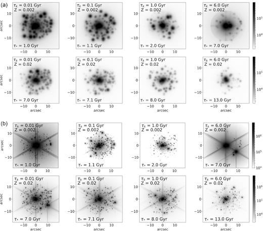
Synthetic spectra along with best-matching spectra from the Pickles library are shown in Fig. D1. Positions of stars within the HCSC as derived by Merritt et al. (2009) at t = 100 × GM_•/V|$^{3}_{k}$| are reproduced in Fig. D2.

Figure D1.

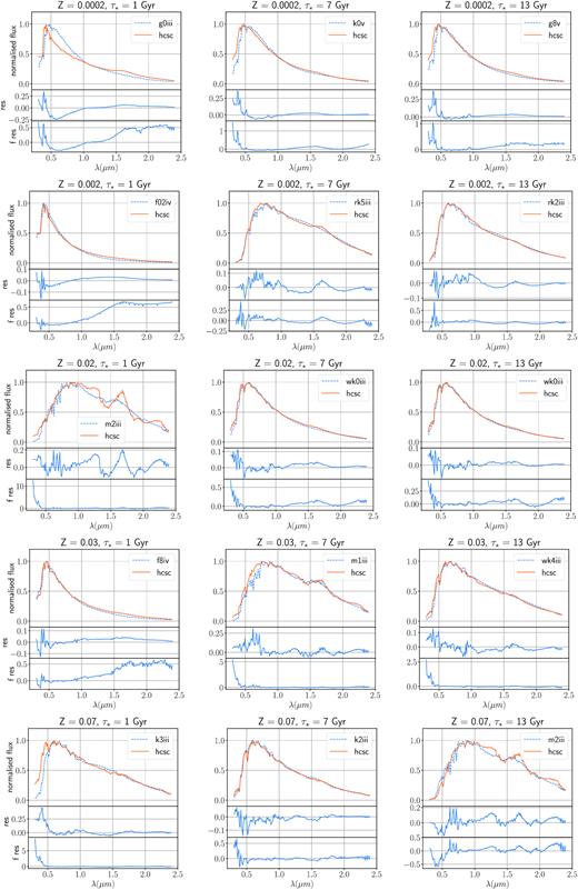
HCSC model spectra with metallicity and stellar population age as indicated in the plot title, and best-matching stellar spectra from the Pickles atlas. Residual (model-star) and fractional residual (model-star)/star are plotted in the bottom panels. Stellar names are indicated following the scheme xxy, with xx the spectral type, and y the luminosity class. The nomenclature rxxy and wxxy refers to metal-rich and metal-weak stars, respectively.

Figure D2.

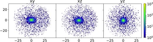
Positions of stars within the HCSC as produced by Merritt et al. (2009) at t = 100 × GM_•/V|$^{3}_{k}$|⁠; the kick was in the −X direction (horizontal negative values in the left-hand and central panels) at t = 0. Units of length are GM_•/V|$^{2}_{k}$|⁠. The colour indicates the number of stars at a given location.