


ABSTRACT
We present Hubble Space Telescope imaging of a pre-explosion counterpart to SN 2019yvr obtained 2.6 yr before its explosion as a type Ib supernova (SN Ib). Aligning to a post-explosion Gemini-S/GSAOI image, we demonstrate that there is a single source consistent with being the SN 2019yvr progenitor system, the second SN Ib progenitor candidate after iPTF13bvn. We also analysed pre-explosion Spitzer/Infrared Array Camera (IRAC) imaging, but we do not detect any counterparts at the SN location. SN 2019yvr was highly reddened, and comparing its spectra and photometry to those of other, less extinguished SNe Ib we derive |$E(B-V)=0.51\substack{+0.27\\ -0.16}$| mag for SN 2019yvr. Correcting photometry of the pre-explosion source for dust reddening, we determine that this source is consistent with a log (L/L⊙) = 5.3 ± 0.2 and |$T_{\mathrm{eff}} = 6800\substack{+400\\ -200}$| K star. This relatively cool photospheric temperature implies a radius of 320|$\substack{+30\\ -50}~\mathrm{ R}_{\odot}$|, much larger than expectations for SN Ib progenitor stars with trace amounts of hydrogen but in agreement with previously identified SN IIb progenitor systems. The photometry of the system is also consistent with binary star models that undergo common envelope evolution, leading to a primary star hydrogen envelope mass that is mostly depleted but still seemingly in conflict with the SN Ib classification of SN 2019yvr. SN 2019yvr had signatures of strong circumstellar interaction in late-time (>150 d) spectra and imaging, and so we consider eruptive mass-loss and common envelope evolution scenarios that explain the SN Ib spectroscopic class, pre-explosion counterpart, and dense circumstellar material. We also hypothesize that the apparent inflation could be caused by a quasi-photosphere formed in an extended, low-density envelope, or circumstellar matter around the primary star.
1 INTRODUCTION
Core-collapse supernovae (SNe) are the terminal explosions of stars with initial mass >8 M⊙ (Burrows, Hayes & Fryxell 1995). This aspect of massive star evolution was empirically confirmed by the discovery of the blue supergiant progenitor of SN 1987A (Podsiadlowski 1993) and subsequent discovery of over two dozen SN progenitors in nearby galaxies (Smartt et al. 2015, and references therein, with more discovered since). The majority of these stars are red supergiant (RSG) progenitors of hydrogen-rich type II SNe (SNe II), although several hydrogen-poor SN IIb progenitor stars, all of which are A–K supergiants, have also been explored in the literature (notably for SNe 1993J, 2008ax, 2011dh, 2013df, and 2016gkg; Aldering, Humphreys & Richmond 1994; Crockett et al. 2008; Maund et al. 2011; Van Dyk et al. 2014; Kilpatrick et al. 2017).
To date, there is only one confirmed example of a progenitor star to a hydrogen-stripped SN Ib; the progenitor of iPTF13bvn in NGC 5608 was initially identified as a compact Wolf–Rayet (WR) star in pre-explosion Hubble Space Telescope (HST) imaging (Cao et al. 2013) and confirmed as the progenitor by its disappearance (Eldridge & Maund 2016; Folatelli et al. 2016). There are numerous upper limits on the progenitor systems of other SNe Ib in the literature (Eldridge et al. 2013). These limits suggest that SN Ib progenitor systems tend to have low optical luminosities, although Eldridge et al. (2013) assume zero host extinction, whereas SNe Ib are known to occur in regions of high extinction (e.g. Drout et al. 2011; Stritzinger et al. 2018).
The transition from hydrogen-rich type II to hydrogen-poor type IIb to hydrogen-free type Ib SNe, and finally to helium-free type Ic SNe is commonly understood as a continuum in final hydrogen (or helium) mass in the envelopes of their progenitor stars (Filippenko 1997; Dessart et al. 2011, 2012, 2015; Yoon et al. 2012; Yoon 2015; Maund & Ramirez-Ruiz 2016). Possible mechanisms that can deplete stellar envelope mass include radiative mass-loss (Heger et al. 2003; Crowther 2007; Smith 2014), eruptive mass-loss (Langer et al. 1994; Maeder & Meynet 2000; Ramirez-Ruiz et al. 2005; Dessart, Livne & Waldman 2010), and mass transfer in binary systems (Woosley et al. 1994; Izzard, Ramirez-Ruiz & Tout 2004; Fryer et al. 2007; Yoon 2017). Stars with higher initial masses or metallicities are predicted to be more stripped at the time of core collapse due to their strong radiative winds (Heger et al. 2003). However, extremely high-mass stars that can efficiently deplete their envelopes have more compact and thus less explodable cores, which is thought to lead to a significant fraction of failed SNe, that is, direct collapse to a black hole with no luminous transient (Burrows et al. 2007; Sukhbold et al. 2016; Murguia-Berthier et al. 2020). In addition, the large relative fraction of stripped-envelope SNe in volume-limited surveys (i.e. SNe Ib and Ic; Li et al. 2011; Shivvers et al. 2017a; Graur et al. 2017a, b) suggests they come from a progenitor channel including stars with initial masses <30 M⊙ (Smith et al. 2011; Eldridge et al. 2013).
Mass transfer in a binary system is therefore an appealing alternative mechanism to strip massive star envelopes as the majority of massive stars are observed to evolve in binaries (Kiminki & Kobulnicky 2012; Sana et al. 2012), and binary interactions can lead to a wide variety of outcomes based on mass ratio, orbital period, and the characteristics of each stellar component (e.g. Wu et al. 2020). In particular, Case B (during helium core contraction; Kippenhahn & Weigert 1967) or Case BB (after core helium exhaustion for a star with previous Case B mass transfer; Delgado & Thomas 1981) mass transfer can remove nearly all of a star’s hydrogen envelope, although this process typically stops before hydrogen is completely depleted (Yoon, Woosley & Langer 2010; Yoon 2015, 2017). Stars with a small amount of hydrogen remaining might also swell up in the latest stages of evolution (Divine 1965; Habets 1986; Götberg, de Mink & Groh 2017; Laplace et al. 2020) and fill their Roche lobes to restart mass transfer. If mass transfer is non-conservative, that is some of the material is not accreted by the companion star, this scenario can lead to dense circumstellar material (CSM) in their local environments. Thus, when the primary star explodes the SN ejecta might encounter and shock this material, producing strong thermal continuum and hydrogen and helium line emission at optical wavelengths (i.e. SN IIn and Ibn features; Vanbeveren et al. 1979; Claeys et al. 2011; Maund et al. 2016; Smith 2017; Yoon, Dessart & Clocchiatti 2017; Götberg et al. 2019). Thus, the final envelope mass, radius, and composition of the star can result in SNe with diverse photometric and spectroscopic properties (James & Baron 2010) ranging from type II to type IIn to type Ic-like evolution.
One prediction from this model of binary mass transfer is that there may be a continuum between SNe with type IIb and Ib-like behaviour, depending on their final hydrogen mass. Dessart et al. (2012) find that progenitor stars with as little as 10−3 M⊙ hydrogen envelope mass would produce an SN whose spectra exhibit broad H α line emission up to 10 d after maximum light (although other studies find the envelope mass can be as large as 0.02–0.03 M⊙ with no H α signature; Hachinger et al. 2012). Stars on either edge of this mass threshold are expected to vary not only in the spectroscopic evolution of their resulting SN but also their appearance in pre-explosion imaging. Above this threshold, spectroscopic evolution should be similar to archetypal SNe IIb such as SN 1993J (Filippenko, Matheson & Ho 1993; Richmond et al. 1994; Woosley et al. 1994), and the progenitor star can inflate to radii >400 R⊙ (Yoon 2017; Laplace et al. 2020). Indeed, the progenitor of SN 1993J was a K-type supergiant with a photospheric radius 300–600 R⊙ (Nomoto et al. 1993; Aldering et al. 1994; Fox et al. 2014). In contrast, stars with final hydrogen-envelope masses low enough that they would be classified as a type Ib SN prior to maximum light are only expected to inflate to radii of at most ∼100 R⊙ (Yoon et al. 2012; Yoon 2015, 2017; Kleiser, Fuller & Kasen 2018; Laplace et al. 2020), and in many cases they remain significantly smaller. This should result in hotter progenitor stars for a given luminosity.
Intriguingly, some SNe Ib exhibit signatures of circumstellar interaction with hydrogen-rich gas weeks to months after explosion, which suggests their progenitor stars (or binary companions) recently released this material from their envelopes. The best-studied example to date is SN 2014C (Milisavljevic et al. 2015; Tinyanont et al. 2016, 2019; Margutti et al. 2017), which was discovered in NGC 7331 at ≈15 Mpc, but several other stripped-envelope SNe with similar evolution have been presented in the literature (e.g. SNe 2001em, 2003gk, 2004dk, 2018ijp, 2019tsf, 2019oys; Chugai & Chevalier 2006; Bietenholz et al. 2014; Chandra 2018; Mauerhan et al. 2018; Pooley et al. 2019; Sollerman et al. 2020; Tartaglia et al. 2020) as well as the initially hydrogen-free superluminous SN iPTF13ehe (Yan et al. 2017). Although non-conservative mass transfer or common envelope ejections have been proposed as the source of this material (Sun, Maund & Crowther 2020), it is still unclear what evolutionary pathways lead to these apparently hydrogen-stripped stars or what exact mechanism causes an ejection timed only years before explosion (up to 1 M⊙ of hydrogen-rich CSM for SN 2014C in Margutti et al. 2017).
Understanding how common stripped-envelope SNe with circumstellar interactions are might aid in ruling out less likely mechanisms, but constraining the exact rate is difficult as few SNe are close and bright enough to follow to late times and stripped-envelope SNe tend to be further extinguished in their host galaxies (Stritzinger et al. 2018). Some SN Ib exhibit clear signatures of circumstellar interaction with helium-rich material at early times (so-called SNe Ibn, with narrow emission lines of helium indicative of interaction between SN ejecta and slow moving, circumstellar helium; Pastorello et al. 2008; Shivvers et al. 2017b), potentially from massive, helium-rich WR stars undergoing extreme mass-loss immediately before explosion (Smith et al. 2017). However, events from this class are rare and there with significant photometric and spectroscopic diversity (Hosseinzadeh et al. 2017). Margutti et al. (2017) analysed 183 SNe Ib and Ic with late-time radio observations and found that 10 per cent exhibit evidence for rebrightening consistent with SN 2014C-like evolution, implying this phenomenon may be relatively common. However, volume-limited samples with light curves beyond 100 d of discovery (when most of these interactions occur; Sollerman et al. 2020) are small (e.g. in Li et al. 2011; Shivvers et al. 2017a), and so there may be an observational bias preventing precise constraints on the intrinsic rate of these interactions in SNe Ib/c.
In this paper, we discuss a progenitor candidate for the SN Ib 2019yvr discovered in NGC 4666 on UTC 2019 December 27 12:30:14 (MJD 58844.521) by the Asteroid Terrestrial impact Last Alert System (ATLAS; Smith et al. 2019).1 We present early-time light curves and spectra of SN 2019yvr demonstrating that it resembles several other SNe Ib and is spectroscopically most similar to iPTF13bvn, albeit with much more line-of-sight extinction than most known SNe Ib. We also note that SN 2019yvr exhibited signatures of circumstellar interaction at >150 d from discovery, with evidence for relatively narrow H α, X-ray, and radio emission at these times (Auchettl et al., in preparation). From this information, we infer that SN 2019yvr is similar to SN 2014C, with early-time type Ib-like evolution but transitioning around 150 d to a light curve powered by shock interaction with CSM at all wavelengths.
NGC 4666 has deep Hubble Space Telescope/Wide Field Camera 3 (HST/WFC3) imaging in F438W, F555W, F625W, and F814W bands (roughly BVRI, respectively) that covers the site of SN 2019yvr 2.6 yr before its explosion (Foley et al. 2016; Shappee et al. 2016; Graur et al. 2018). Compared with limits on the progenitor stars of other SNe Ib in the literature (Eldridge et al. 2013) as well as the detection of the progenitor star of iPTF13bvn (Cao et al. 2013), these data are among the deepest pre-explosion imaging for any SN Ib. We compare follow-up adaptive optics-fed imaging to the pre-explosion HST images and identify a single progenitor candidate and compare the progenitor candidate photometry to single- and binary-star models in Section 4. Finally, we discuss the inferred candidate properties in the context of SN 2019yvr and models of stripped-envelope SNe in Section 5 and our final conclusions in Section 6.
Throughout this paper, we assume a distance to NGC 4666 of m − M = 30.8 ± 0.2 mag (14.4 ± 1.3 Mpc) derived from the light curve of the type Ia SN ASASSN-14lp also observed in this galaxy (Shappee et al. 2016). We assume a redshift to NGC 4666 of z = 0.005 080 (Allison, Sadler & Meekin 2014) and Milky Way reddening E(B − V) = 0.02 mag (Schlafly & Finkbeiner 2011).
2 OBSERVATIONS
2.1 High-resolution pre-explosion images of the SN 2019yvr explosion site
We analysed HST/WFC3 imaging of NGC 4666 obtained from the Mikulski Archive for Space Telescopes.2 These data were observed over five epochs from 2017 April 21 to August 7 (Cycle 24, GO-14611, PI Graur; see Table 2), corresponding to 980–872 d (2.68–2.39 yr) before discovery of SN 2019yvr. Using our analysis code hst123,3 we downloaded every HST image covering the explosion site of SN 2019yvr. These comprised WFC3/UVIS flc frames calibrated with the latest reference files, including corrections for bias, dark current, flat-fielding, bad pixels, and geometric distortion. We optimally aligned each image using TweakReg with 1000–2000 sources per frame and resulting in frame-to-frame alignment with 0.1–0.2 pix (0.005–0.010 arcsec) root-mean-square dispersion. We then drizzled all images in each band and epoch with astrodrizzle. With the drizzled F555W frame as a reference, we obtained photometry in the flc frames of every source on the same chip as the SN 2019yvr explosion site using dolphot (Dolphin 2016). Our dolphot parameters followed the recommended settings for WFC3/UVIS4 as described in hst123. We show a colour image constructed from the F814W, F555W, and F438W frames obtained on 2017 June 13 in Fig. 1.
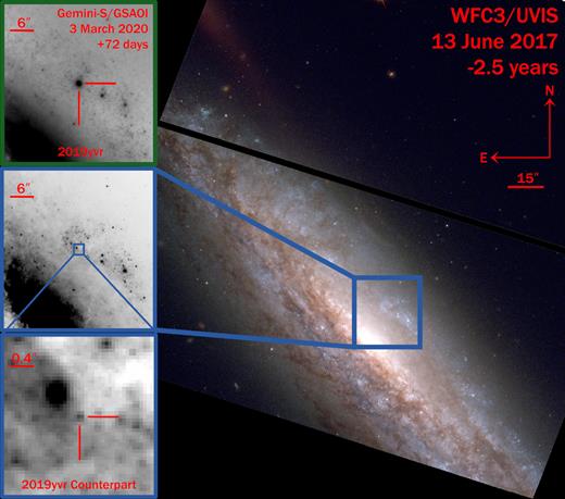
(Right) Hubble Space Telescope imaging of the SN 2019yvr explosion site from 2.5 yr before discovery consisting of F814W (red), F555W (green), and F438W (blue). All images are oriented with north up and east to the left. The colour image on the right is 165 arcsec × 165 arcsec, while the left-upper and left-middle images are 38.8 arcsec × 38.8 arcsec, and the left-lower image is 2.4 arcsec × 2.4 arcsec. The blue box denotes the approximate location of SN 2019yvr. (Upper left): Gemini-S/GSAOI H-band image of SN 2019yvr obtained 67 d after discovery of the transient. The image is centred on the location of SN 2019yvr. (Middle left): Pre-explosion F555W imaging of NGC 4666 showing the same location as the upper left. (Lower left): Pre-explosion F555W imaging zoomed into the blue box from the middle left. The location of the SN 2019yvr progenitor candidate derived from our Gemini-S/GSAOI imaging is shown as red lines, which agrees with the location of a single point source as discussed in Section 4.1.
In addition, multiple epochs of Spitzer/Infrared Array Camera (IRAC) imaging of NGC 4666 were obtained from 2005 January 4 to 2014 September 25, or roughly 15.0–5.3 yr before discovery of SN 2019yvr. There was a single epoch of Channel 4 (7.9 µm) imaging that observed NGC 4666 (AOR 21999872; PI Rieke), but no Spitzer/IRAC observations cover NGC 4666 in Channel 3 (5.7 µm). We downloaded the basic calibrated data (cbcd) frames and stacked them using our custom Spitzer/IRAC pipeline based on the photpipe imaging and reduction pipeline (Rest et al. 2005; Kilpatrick et al. 2018a). The IRAC frames were stacked and regridded to a pixel scale of 0.6 arcsec pixel−1 using SWarp (Bertin 2010). We performed photometry on the stacked frames using DoPhot (Schechter, Mateo & Saha 1993) and calibrated our data with Spitzer/IRAC instrumental response (for the cold and warm missions where appropriate; Hora et al. 2012) in the stacked frames. Based on the PSF width and average sky background, the average depth of the Spitzer/IRAC images is approximately (3σ; AB mag) 24.3, 24.6, and 23.0 mag at 3.6, 4.5, and 7.9 µm, respectively.
2.2 Adaptive optics imaging of SN 2019yvr
We observed SN 2019yvr in H band on 2020 March 8, or 72 d after discovery, with the Gemini-South telescope from Cerro Pachón, Chile and the Gemini South Adaptive Optics Imager (GSAOI; McGregor et al. 2004). We used the Gemini Multi-conjugate Adaptive Optics System (GeMS; Rigaut et al. 2014) with the Gemini South laser guide star system to perform adaptive optics corrections over the GSAOI field of view (85 arcsec × 85 arcsec) and using SN 2019yvr itself to perform tip-tilt corrections. We alternated observations between a field covering SN 2019yvr and a relatively empty patch of sky 4 arcmin to the south in an on–off pattern, totalling 1005 s of on-source exposure time over 39 frames. Using the GSAOI reduction tools in IRAF,5 we flattened the images with a flat-field frame constructed from observations of a uniformly illuminated screen in the same filter and instrumental setup with unilluminated frames of the same exposure time to account for bias and dark current. We then subtracted the sky frames from our on-source frames.
GSAOI has a well-understood geometric distortion pattern (Neichel et al. 2014). We used this distortion pattern to resample each on-source frame to a corrected grid, aligned the individual exposures, and constructed a mosaic from each amplifier in the on-source frames with the GSAOI tool disco-stu.6 Finally, we stacked the individual frames with SWarp using an inverse-variance weighted median algorithm and scaling each image to the flux of isolated point sources observed in every on-source exposure. The final stacked frame is shown in the upper-left inset of Fig. 1 centred on SN 2019yvr.
2.3 Photometry of SN 2019yvr
We observed SN 2019yvr with the Swope 1.0-m telescope and Direct/4K × 4K imager at Las Campanas Observatory, Chile from 2020 January 1 to 28 in uBVgri. Following reduction procedures described in Kilpatrick et al. (2018a), we performed all image processing and photometry on the Swope data using photpipe (Rest et al. 2005). The final BVgri photometry of SN 2019yvr were calibrated using PS1 standard sources (Flewelling et al. 2020) observed in the same field as SN 2019yvr and transformed into the Swope natural system following the Supercal method (Scolnic et al. 2015). In u band, we calibrated our images using SkyMapper standards (Onken et al. 2019) in the same frame as SN 2019yvr.
We also observed SN 2019yvr with the Las Cumbres Observatory (LCO) Global Telescope Network 1-m telescopes from 2019 December 29 to 2020 February 3 with the Sinistro imagers and in g′r′i′. We obtained the processed images (from the banzai pipeline; McCully et al. 2018) from the LCO archive and processed them in photpipe, registering each image to a corrected grid with SWarp (Bertin 2010) and performing photometry on the individual frames with DoPhot (Schechter et al. 1993). We then calibrated the g′r′i′ photometry using gri PS1 standards.
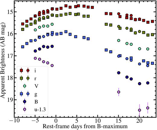
All Swope and LCO photometry are listed in Table A1 and shown in Fig. 2. We estimated the time of maximum light in V band by fitting a low-order polynomial to the overall light curve and derive a time of V-band maximum light at MJD 58853.64 (2020 January 5.64). Detailed modelling of the light curves and inferred explosion parameters will be presented by Auchettl et al. (in preparation).
2.4 Spectroscopy and classification of SN 2019yvr
We triggered spectroscopic observations of SN 2019yvr on the Faulkes-North 2-m telescope at Haleakalā, Hawaii with the FLOYDS spectrograph (Program NOAO2020A-008, PI Kilpatrick). The spectrum was observed on 2020 January 2 roughly 5 d after the initial discovery report from ATLAS and 3 d before SN 2019yvr reached V-band maximum. The observation was a 1500-s exposure at an average airmass of 1.35 and under near-photometric observing conditions. We reduced the spectrum following standard procedures in IRAF, including corrections for telluric absorption and correcting the wavelength solution for atmospheric diffraction using the sky lines. The final reduced spectrum is shown in Fig. 3.
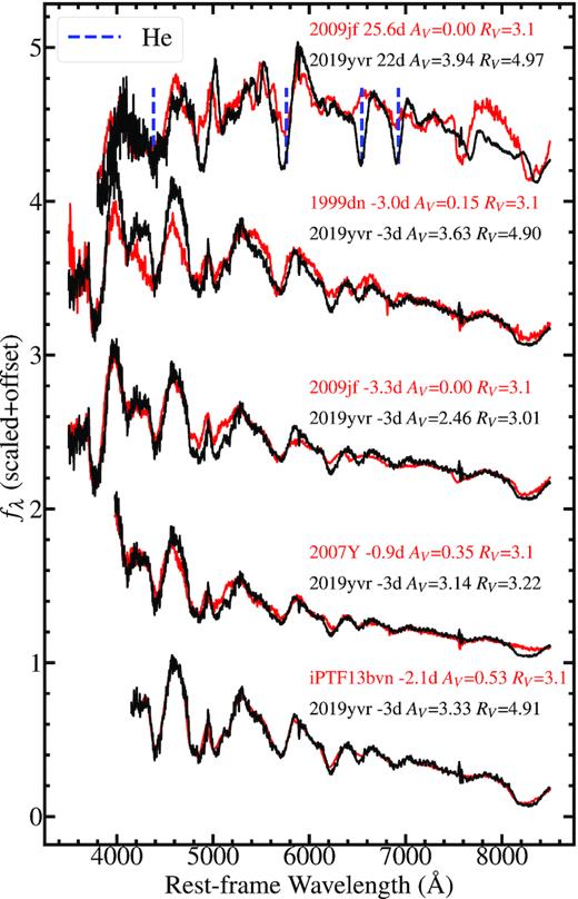
Our spectra of SN 2019yvr (black) with comparison to other SNe Ib (red). All dates are indicated with a ‘d’ with respect to V-band maximum light. The comparison spectra have been dereddened for Milky Way extinction based on values in Schlafly & Finkbeiner (2011) and dereddened for host extinction based on values in Deng et al. (2000); Benetti et al. (2011) (for SN 1999dn), Stritzinger et al. (2009) (for SN 2007Y), Valenti et al. (2011) (for SN 2009jf), and Srivastav et al. (2014) (for iPTF13bvn). We removed the recessional velocity for z = 0.005 080 from the SN 2019yvr spectra and dereddened them following the methods given in Section 3.3. The best-fitting extinction and RV parameter are given next to each SN 2019yvr spectrum. We highlight lines of He i at λλ4471, 5876, 6678, and 7065, which are present in both epochs, demonstrating that SN 2019yvr is a SN Ib.
We also observed SN 2019yvr on the Keck-I 10-m telescope on Maunakea, Hawaii with the Low-Resolution Imaging Spectrograph (LRIS; Program 2019B-U169, PI Foley) on 27 January 2020, approximately 22 d after V-band maximum as seen from our light curve. The observation was a 180-s exposure obtained during morning twilight at an average airmass of 1.16 and under near-photometric conditions. We reduced these data using a custom pyraf-based LRIS pipeline (Siebert et al. 2020),7 which accounts for bias-subtraction, flat-fielding, amplifier crosstalk, background and sky subtraction, telluric corrections using a standard observed on the same night and at a similar airmass, and order combination. The final combined spectrum is shown in Fig. 3.
Our spectra reveal characteristic SN Ib features with strong, broad absorption lines of He i λλ4471, 5876, 6678, and 7065 (Fig. 3). These features and the lack of any apparent Balmer line emission indicate that SN 2019yvr is a typical SN Ib, and our comparisons to other SNe Ib such as iPTF13bvn (Srivastav, Anupama & Sahu 2014) suggest it is well matched to this spectroscopic class as a whole. From the spectrum obtained at 3 d before maximum light, we infer a velocity from Ca absorption of 22 000 km s−1. We also note prominent lines of Na i D absorption at the redshift of NGC 4666 (z = 0.005 080). We do not detect evidence for any diffuse interstellar bands (DIBs) that can be used to derive line-of-sight extinction in the regime of large Na i D column densities (e.g. Phillips et al. 2013). The complete spectroscopic evolution of SN 2019yvr will be addressed by Auchettl et al. (in preparation).
3 EXTINCTION TOWARDS SN 2019yvr AND ITS PROGENITOR SYSTEM
Stripped-envelope SNe Ib are known to occur in regions of high extinction in their host galaxies (Drout et al. 2011; Galbany et al. 2016a, b; Stritzinger et al. 2018). However, if there is significant extinction due to dust in the circumstellar environment of SN 2019yvr, it may be variable between the time the HST images and imaging and spectra of SN 2019yvr were obtained. Moreover, we have no a priori constraint on the dust composition or gas-to-dust ratio in the local interstellar environment of SN 2019yvr, which is a major factor in understanding the magnitude of extinction at all optical wavelengths.
Based on the relatively low Milky Way reddening of E(B − V) = 0.02 mag and the fact that SN 2019yvr exhibited red colours (Fig. 2) and strong Na i D absorption, we infer that SN 2019yvr and its progenitor system are heavily extinguished by its host’s interstellar and/or its own circumstellar environment. Moreover, if we do not correct for any additional extinction, the V-band light curve would peak at only −15.1 mag. This is extremely faint compared with other SNe Ib/c and suggests AV > 1 mag (Drout et al. 2011; Stritzinger et al. 2018, although this inference may be affected by Malmquist bias if known samples of SNe Ib are not representative of the overall luminosity function).
Throughout the remainder of this section, we consider contextual information about the host galaxy NGC 4666, observations of SN 2019yvr, and the extinction properties of circumstellar dust around analogous stripped-envelope SN Ib progenitor systems in order to infer the total extinction to the SN 2019yvr progenitor system. Our goal is to derive a V-band extinction AV and reddening law parameter RV that can be used to estimate the total extinction in the HST bandpasses as observed in pre-explosion data.
3.1 Extinction inferred from Na i D
One quantity that is correlated with line-of-sight reddening in both SNe (Stritzinger et al. 2018) and quasars (Poznanski, Prochaska & Bloom 2012) is the equivalent width of Na i D. We detect Na i D in our 2019yvr LRIS spectrum with equivalent width of 4.2 ± 0.2 Å, which is significantly larger than the maximum Na i D equivalent width (2.384 Å) from the quasars used to derive the reddening relation in Poznanski et al. (2012), implying that we might overestimate the total extinction by applying their relation. Indeed, our measured Na i D equivalent width combined with the Poznanski et al. (2012) relation would indicate SN 2019yvr has a light of sight E(B − V) > 1000 mag, which is impossible for any extragalactic optical transient. This finding could be due in part to saturation in the Na i D line for the original sample of quasars in Poznanski et al. (2012), which prevents an accurate measurement of the true column of Na i D as a function of the total column optical extinction. We infer that the Poznanski et al. (2012) relationship is not accurate in this high extinction and large Na i D equivalent width regime where we find SN 2019yvr (consistent with findings in Stritzinger et al. 2018).
If we instead use the relation between AV and Na i D equivalent width in Stritzinger et al. (2018), which was derived specifically from SN Ib/c colour curves, we find SN 2019yvr has a line-of-sight extinction AV = 3.4 ± 0.6 mag. However, we emphasize that the validity of this relationship at such large equivalent widths has not been tested, and, more broadly, there is significant scatter in the correlation between Na i D equivalent width and optical extinction (Phillips et al. 2013). Therefore, we turn to other extinction indicators to better estimate the line-of-sight extinction.
3.2 Extinction inferred from SN 2019yvr spectra
Spectra and light curves of SNe Ib similar to SN 2019yvr can be used to constrain its line-of-sight extinction. As host extinction is a dominant systematic uncertainty in estimating intrinsic stripped-envelope SN colours, any differences in broad-band colours between SNe at similar epochs can be attributed to extinction. Here, we compare our SN 2019yvr spectra to those of other SNe Ib applying a Cardelli, Clayton & Mathis (1989) extinction law with variable E(B − V) and RV to deredden our SN 2019yvr until they closely match.
Our best-fitting parameters for V-band extinction (AV) and RV inferred for SN 2019yvr based on matching to template spectra as shown in Fig. 3 and described in Section 3.2. As in Fig. 3, the epoch of each SN 2019yvr and template spectrum is given in days with respect to V-band maximum light. χ2 is given in units of reduced |$\chi ^{2}/\chi ^{2}_{\mathrm{min}}$|. We give parameters for each template spectrum used and the inverse χ2-weighted average for AV and RV. However, see caveats in Section 3.2.
| Epoch | Template (epoch) | AV,Temp. | AV,19yvr | RV,19yvr | χ2 |
|---|---|---|---|---|---|
| (d) | (d) | (mag) | (mag) | ||
| −3 | iPTF13bvn (−2.1) | 0.53 | 3.33 ± 0.24 | 4.91 ± 0.37 | 1.00 |
| −3 | SN 2007Y (−0.9) | 0.35 | 3.14 ± 0.29 | 3.22 ± 0.41 | 4.40 |
| −3 | SN 2009jf (−3.3) | 0.00 | 2.46 ± 0.32 | 3.01 ± 0.40 | 4.08 |
| −3 | SN 1999dn (−3.0) | 0.15 | 3.62 ± 0.24 | 4.90 ± 0.49 | 5.31 |
| +22 | SN 2009jf (+25.6) | 0.00 | 3.94 ± 0.38 | 4.97 ± 0.56 | 17.42 |
| Mean | 3.3 ± 0.4 | 4.1 ± 0.9 |
As reported in Section 2.4, our SN 2019yvr spectra correspond to approximately −3 and +22 d relative to V-band maximum. For the latter spectrum, only SN 2009jf had a spectrum sufficiently close in V-band epoch to perform a robust comparison between spectral shape. Thus, while the best-fitting cases all correspond to the early-time spectrum, our second epoch serves to validate the results of this analysis. In this way, we derive a line-of-sight extinction to SN 2019yvr of AV = 2.4–3.9 mag, although most of our best-fitting values are around AV = 3.2–3.6 mag. These values are consistent with Na i D, but there is significant scatter in AV, implying that there are systematic uncertainties in our method.
3.3 Extinction inferred from SN 2019yvr colour curves
We further investigate the interstellar host reddening using colour curve templates from Stritzinger et al. (2018) and compare to our Swope and LCO colour curves of SN 2019yvr (Fig. 4). Using a Cardelli et al. (1989) reddening law, we vary the values of AV and RV in order to derive colour corrections due to interstellar reddening. We apply these corrections to our B − g, B − V, g − r, and g − i colour curves to find the best fit with Stritzinger et al. (2018) template colours as shown in Fig. 4. The best-fitting values are quantified with respect to the summed χ2 values in B − g, B − V, g − r, and r − i and across all epochs. The final reduced χ2 value for different values of AV and RV is shown in Fig. 5.
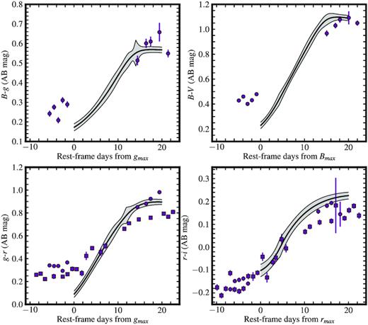
Colour curves of SN 2019yvr corrected for Milky Way and interstellar host extinction (with AV = 2.4 mag and RV = 4.7) as discussed in Section 3.3. Circles correspond to our Swope photometry while squares are for LCO photometry. We overplot templates for extinction-corrected SN Ib colour curves from Stritzinger et al. (2018) as black lines with the 1σ uncertainties in each template as a grey shaded region.
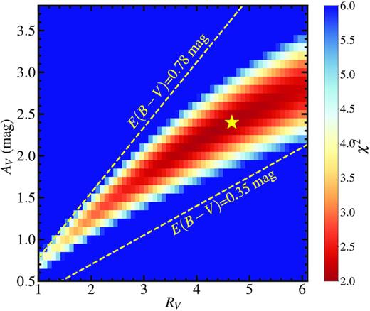
χ2 values as a function of assumed interstellar V-band extinction AV and reddening law parameter RV and comparing SN 2019yvr colours to the colour templates in Section 3.3 and Fig. 4. The best-fitting extinction parameters are AV = 2.4 mag and RV = 4.7 (yellow star) with an implied a best-fitting E(B − V) = 0.51 mag. The yellow dashed lines show the 1σ best-fitting limits of E(B − V).
We find the best-fitting values using our colour curve matching are |$A_{V}=2.4\substack{+0.7\\-1.1}$| mag and |$R_{V}=4.7\substack{+1.3\\-3.0}$| and implying a best-fitting |$E(B-V)=0.51\substack{+0.27\\-0.16}$| mag. The value of RV is limited at the high end by our boundary condition that RV < 6.0. Based on well-measured values of RV for SN host galaxies (e.g. the wide variety of SN Ia hosts presented in Amanullah et al. 2015), which tend to have 1.3 < RV < 3.6, we infer that our prior RV < 6.0 is a conservative upper bound on realistic values of the reddening law parameter.
3.4 Final extinction value adopted for SN 2019yvr
Overall, the level of extinction inferred from our spectral analysis is consistent with our estimate from the V-band light curve as well as the value inferred from the Stritzinger et al. (2018) Na i D relation. While the latter relationship diverges significantly at large extinction values (also similar to Poznanski et al. 2012), we infer from the agreement between these three estimates that the line-of-sight host extinction inferred for SN 2019yvr is close to the value inferred from our spectral and colour curve analyses. However, the colour curve analysis involves more independent measurements of the SN 2019yvr optical spectrum, and this analysis has been validated for several SNe Ib by Stritzinger et al. (2018). Thus, although there is agreement between all of our methods, we infer that |$A_{V}=2.4\substack{+0.7\\-1.1}$| mag and |$R_{V}=4.7\substack{+1.3\\-3.0}$| is most representative of the line-of-sight extinction to SN 2019yvr, and we use these values and our χ2 distribution on extinction in Fig. 5 below.
However, the critical question to the analysis below is how much extinction did the SN 2019yvr progenitor star experience? While it is reasonable to assume that the interstellar host extinction inferred from SN 2019yvr would be the same as the extinction that its progenitor star experienced (especially on the 2.4–15.0 yr time-scale of our pre-explosion data), there could be additional sources of extinction present when the pre-explosion data were obtained to which our SN 2019yvr observations are not sensitive or vice versa. In particular, circumstellar dust could have been present in the pre-explosion environment but vapourized soon after explosion, or else there could be material ejected by the progenitor star very soon before explosion that was not present when the HST or Spitzer data were obtained. Below we consider both scenarios and the effects of circumstellar material and extinction on our overall data set.
3.5 Possibility of more circumstellar extinction 2.6 yr prior to core collapse
All massive stars exhibit winds that pollute their environments with gas and dust (Smith 2014), and this material can lead to significant circumstellar extinction when the wind is dense, clumpy, and relatively cool. Thus it is possible that the SN 2019yvr progenitor star experienced significant circumstellar extinction from a shell of dust that was vapourized before it could be observed in the SN. Auchettl et al. (in preparation) find evidence for a significant mass of hydrogen-rich CSM from H α, X-ray, and radio emission. Rebrightening in the light curve of SN 2019yvr beginning >150 d after discovery suggests that this material is in a shell likely at >1000 au from the progenitor star, thus ejected years or decades before core collapse.
The question we address here is whether there could also be material closer to the progenitor star that contributes to circumstellar extinction but was vapourized soon after core collapse, implying that the line-of-sight extinction estimated above underestimates the extinction at the time of the HST observations. There is no obvious sign of any such material, for example, in evolution of the Na i D profile or excess emission in early-time light curves and spectra.
Dust geometries and properties most likely to be associated with circumstellar extinction due to material close (2–10× the photospheric radius as in Kochanek, Khan & Dai 2012) to the progenitor star but unconstrained by our SN 2019yvr observations can be probed with our mid-infrared Spitzer/IRAC limits. Assuming this material was present on the time-scale of the IRAC observations, we model an optically thin shell of dust to our limits of 22.8, 23.1, and 21.5 mag in IRAC bands 1, 2, and 4, respectively (see Section 4.1 for a discussion of the IRAC limits). A warm shell of gas and dust (T > 200 K) would result in bright mid-infrared emission even in cases where it is relatively compact (<1 au). Following analysis in Kilpatrick et al. (2018a), Kilpatrick & Foley (2018), and Jacobson-Galán et al. (2020), we modelled optically thin shells of silicate dust with grain sizes >0.1 µm and a range of temperatures from 200 to 1500 K. At hotter temperatures, the dust would likely sublimate and thus would not exhibit the same extinction properties or attendant mid-infrared emission. Similarly, a shell at large distances from its progenitor star might be so cool that it does not emit significant flux at <10 µm where our IRAC data probe, even if it has a large mass.
The dust mass limits we derive are strongly temperature dependent, with the coolest temperatures yielding the weakest limits on mass (Md < 9 × 10⁻⁴ M⊙ and Ld < 4 × 10⁴ L⊙ at 200 K) whereas hotter dust leads to relatively strong limits on dust mass (Md < 2 × 10⁻⁸ M⊙ and Ld < 9 × 10⁴ L⊙ at 1500 K). We used the 0.1 µm silicate dust grain opacities from Fox et al. (2010, 2011) to calculate these limits. Assuming the same dust grain composition, we approximate the limits on optical depth in V band as τV = ρκVrdust, where rdust is the implied blackbody radius of the dust shell, |$\rho \approx M_{\mathrm{ d}}/(4/3 \pi r_{\mathrm{dust}}^{3})$|, and κV is the opacity in V band. Under these assumptions, the optical depth must be τV < 3–187, with the strongest limits again coming from the hottest dust temperatures.
Approximating AV = 0.79τV as in Kochanek et al. (2012) and Kilpatrick & Foley (2018), these limits are not constraining on the total circumstellar extinction due to a compact dust shell. Indeed, circumstellar dust absorption could be the dominant source of extinction in the SN 2019yvr progenitor system, but we would have no contextual information from the pre-explosion Spitzer/IRAC photometry to constrain the magnitude of that extinction.
The strongest argument against such a compact, warm shell of gas, and dust is the lack of any hydrogen or helium emission associated with circumstellar interaction in early-time spectra or any near-infrared excess in the photometry as shown in Figs 3 and 2. However, these arguments are biased by the epoch of the first observations. SN 2019yvr had a reported discovery on 2019 December 27 by ATLAS with the last previous non-detection occurring on 2019 December 11 at >18.6 mag in o band (Smith et al. 2019). Subsequent non-detection reports by the Zwicky Transient Facility give a more constraining non-detection in g band at >19.5 mag on 2019 December 13.9 However, this still allows for 14 d when SN 2019yvr could have interacted with CSM in its immediate environment. Although the first spectrum of SN 2019yvr did not exhibit evidence for flash ionization or narrow emission lines due to CSM interaction, this would not be surprising if the explosion was already more than several days old (e.g. flash ionization lasted for <6 d for the type IIb SN 2013cu; Gal-Yam et al. 2014). Deeper and higher cadence early-time observations and pre-explosion limits, especially from high-resolution, near-, and mid-infrared imaging, would have been needed to provide meaningful constraints on the presence and total mass of such material.
3.6 Possibility of less circumstellar extinction 2.6 yr prior to core collapse
There is strong evidence for circumstellar interaction around SN 2019yvr in optical spectra, radio, and X-ray detections starting around 150 d after discovery (Auchettl et al., in preparation). The development of narrow Balmer lines at these late times indicates this material is hydrogen rich. A delayed interaction points to a shell of material at a large projected separation from the progenitor (≈1000 au assuming an SN shock velocity of ≈10 000 km s−1).
A key consideration above is whether this CSM was present at the time of the HST observations or if it was ejected in the subsequent 2.6 yr before core collapse. In the latter case, any dust synthesized in the CSM would not be present in the HST data and thus |$A_{V}=2.4\substack{+0.7\\-1.1}$| mag would be an overestimate of the extinction affecting any emission we detect in pre-explosion data.
Based on the HST observations and follow up data of the SN, we cannot constrain this scenario. However, one prediction from this scenario would be an intermediate-luminosity transient associated with an extreme mass-loss episode over this time. We analysed this location of the sky and found no luminous counterparts in pre-explosion imaging from the ASAS-SN Sky Patrol10 (Shappee et al. 2014; Kochanek et al. 2017) or the Catalina Surveys Data Release 2 (Drake et al. 2009), but these limits only extend to <13 mag given contamination from the bright center of NGC 4666. Thus we cannot provide a meaningful estimate on any such CSM, but we consider the possibility that AV < 2.4 mag in our analysis of pre-explosion counterparts in Sections 4 and 5 below. In general, we assume that the extinction inferred from SN 2019yvr is the same between the epoch of HST observations and the time of explosion. Overall, we consider |$A_{V}=2.4\substack{+0.7\\-1.1}$| mag and |$R_{V}=4.7\substack{+1.3\\-3.0}$| to represent the total line-of-sight extinction to the SN 2019yvr progenitor system at the time the pre-explosion HST imaging was obtained.
4 THE PROGENITOR CANDIDATE TO SN 2019YVR
4.1 Aligning adaptive optics and pre-explosion imaging
We obtained positions for 114 point sources in our GSAOI adaptive optics image using sextractor (Bertin & Arnouts 1996) and compared these to the positions of the same sources in the F555W HST/WFC3 image as obtained in dolphot. From these common sources, we derived a coordinate transformation solution from GSAOI→HST. We also derived the systematic uncertainty in this transformation by splitting our sample of common astrometric sources in half, re-deriving the coordinate transformation, and then comparing the offset between the remaining HST sources and their positions from our GSAOI image and transformation. Repeating this procedure, we are able to derive an average systematic offset between our GSAOI and HST sources. We assume the root-mean-square of these offsets dominates the error in our astrometric solution, which we find is σα = 0.16 WFC3/UVIS pixels (0.008 arcsec) and σδ = 0.18 WFC3/UVIS pixels (0.009 arcsec).
The position of SN 2019yvr in our GSAOI image corresponds to a single point source in the WFC3/UVIS imaging to a precision of 0.1 WFC3/UVIS pixels (≈0.6σ as the uncertainty on the position of this source from our GSAOI is negligible). We detect this source in the drizzled F555W image at 34σ significance, and there are no other sources at the >5σ level within a separation of 0.27 arcsec or 30 times the astrometric uncertainty. Our WFC2/UVIS photometry is listed in Table 2.
HST WFC3/UVIS photometry of the SN 2019yvr progenitor candidate. All magnitudes are on the AB system.
| MJD | Filter | Exposure (s) | Magnitude | Uncertainty |
|---|---|---|---|---|
| WFC3/UVIS photometry of 2019yvr progenitor candidate | ||||
| 57864.06972 | F438W | 1140 | 26.2028 | 0.2207 |
| 57864.11750 | F625W | 1134 | 24.8352 | 0.0466 |
| 57864.17879 | F555W | 1200 | 25.4011 | 0.0720 |
| 57864.24510 | F814W | 1152 | 24.1778 | 0.0498 |
| 57890.23024 | F555W | 1143 | 25.1599 | 0.0612 |
| 57890.24828 | F625W | 1140 | 24.8008 | 0.0443 |
| 57917.36677 | F438W | 1140 | 26.3646 | 0.4810 |
| 57917.39478 | F625W | 1134 | 24.9420 | 0.0538 |
| 57917.43295 | F555W | 1200 | 25.5264 | 0.0853 |
| 57917.46140 | F814W | 1152 | 24.3412 | 0.0588 |
| 57944.68250 | F555W | 1143 | 25.2253 | 0.0621 |
| 57944.75022 | F625W | 1140 | 24.8760 | 0.0478 |
| 57972.22031 | F438W | 1140 | 25.9439 | 0.2410 |
| 57972.23837 | F625W | 1134 | 25.0531 | 0.0559 |
| 57972.28531 | F555W | 1200 | 25.4908 | 0.0829 |
| 57972.30377 | F814W | 1152 | 24.2492 | 0.0575 |
| Average photometry | ||||
| 57917.88560 | F438W | 3420 | 26.1382 | 0.1622 |
| 57904.13112 | F555W | 5886 | 25.3512 | 0.0319 |
| 57917.74983 | F625W | 5682 | 24.8971 | 0.0221 |
| 57918.00342 | F814W | 3456 | 24.2533 | 0.0319 |
We also examined the position of SN 2019yvr in pre-explosion Spitzer/IRAC imaging. Using the same alignment method as above, we determined the location of SN 2019yvr in the Spitzer/IRAC stacked images using our GSAOI image of SN 2019yvr. Our alignment uncertainty is typically σ ≈ 0.2 IRAC pixels (0.12 arcsec) from GSAOI→IRAC in each channel. We found no evidence of a counterpart in any epoch or the cumulative, stacked pre-explosion frames. Therefore, we place an upper limit on the presence of a pre-explosion counterpart in the stacked IRAC frames by injecting and recovering artificial stars at the location of SN 2019yvr and using the native IRAC point response function for each channel. Our pre-explosion limits for IRAC are reported in Table 3.
IRAC limits on the presence of a pre-explosion counterpart to SN 2019yvr progenitor candidate. All magnitudes are on the AB system.
| Average MJD | Wavelength | Exposure | Limit |
|---|---|---|---|
| (µm) | (s) | (mag) | |
| Spitzer/IRAC pre-explosion limits | |||
| 57917.88560 | 3.6 | 1530.0 | >22.8 |
| 57904.13112 | 4.5 | 1864.8 | >23.1 |
| 57918.00342 | 7.9 | 278.0 | >21.5 |
| Average MJD | Wavelength | Exposure | Limit |
|---|---|---|---|
| (µm) | (s) | (mag) | |
| Spitzer/IRAC pre-explosion limits | |||
| 57917.88560 | 3.6 | 1530.0 | >22.8 |
| 57904.13112 | 4.5 | 1864.8 | >23.1 |
| 57918.00342 | 7.9 | 278.0 | >21.5 |
4.2 The nature of the HST counterpart to SN 2019yvr
Stripped-envelope SNe are known to occur in the brightest, highest extinction, and highest metallicity regions of their host galaxies (Galbany et al. 2016a, b). The iPTF13bvn progenitor system was identified in a relatively uncrowded region of NGC 5086 (Cao et al. 2013) and subsequently confirmed as the actual progenitor by its disappearance (Eldridge & Maund 2016; Folatelli et al. 2016), but in general SNe Ib/c are found in crowded regions of their host galaxies (when the surrounding environment can be resolved, as in Eldridge et al. 2013). For example, the candidate progenitor system of the stripped-envelope SN Ic 2017ein was in an environment with several other luminous sources (Kilpatrick et al. 2018b). This fact and the counterpart’s high optical luminosity suggest it may in fact have an unresolved star cluster or a chance coincidence.
The progenitor candidate is point-like in all pre-explosion HST data. The source does not appear extended in any of the WFC3/UVIS frames, with dolphot average sharpness= −0.02, roundness= 0.36, and classified as a bright star, which is consistent with a circular point source at WFC3/UVIS resolution. The source is not blended with any other nearby sources and has an average crowding = 0.09. Therefore, we conclude that the candidate counterpart is consistent with being a single, isolated point source in all of our images.
One possible scenario is that the candidate source is dominated by emission from multiple stars in a single system or open cluster (similar to those in Bastian et al. 2005; Gieles et al. 2006; Gieles & Portegies Zwart 2011). The PSF size of HST/WFC3 in F555W is ≈0.067 arcsec, or 4.7 pc at the distance of NGC 4666. Many open clusters are smaller than this, and might be so compact as to resemble a point source. The F555W (roughly V band) absolute magnitude we infer for this source is −7.8 mag (assuming AV = 2.4 mag), which would be extremely low luminosity for the population of clusters in Gieles et al. (2006). Thus, while we cannot currently rule out the possibility that the source is a cluster we find it much more likely that the source is dominated by emission from a single star or star system associated with SN 2019yvr.
We estimate a single-trial probability of chance coincidence by considering that there are 3281 sources (of any type) detected at >5σ in a 10 arcsec region surrounding the candidate SN 2019yvr counterpart in any of the HST frames. Thus, at most 6.7 arcsec2 or 2 per cent of this region is subtended by area within 3σ (astrometric uncertainty) of any source, which is a conservative upper limit on the probability of chance coincidence between the counterpart and SN 2019yvr. We find it is unlikely that SN 2019yvr coincides with this source by chance, although we acknowledge that this scenario cannot be ruled out definitively before we demonstrate that the source has disappeared (as in the case of iPTF13bvn; Eldridge & Maund 2016; Folatelli et al. 2016).
Given that SN 2019yvr coincides with a single, bright source, that source is point-like and isolated from nearby sources, and the relatively low likelihood of a chance coincidence, we consider this source to be a credible progenitor candidate to SN 2019yvr. Below we assume that this object is dominated by emission from a single stellar system that hosted the SN 2019yvr progenitor star.
4.3 Photometric properties of the pre-explosion counterpart
We show the light curve of the SN 2019yvr progenitor candidate at times relative to explosion in Fig. 6. The source is relatively stable with at most 0.47 mag peak-to-peak variability (corresponding to 3.4σ) in F555W over a baseline of 110 d. Thus, we infer that the progenitor candidate did not exhibit any extreme variability with constant flux at the <0.24 mag level in all bands. This suggests that if the counterpart is a star, it was not in an eruptive or any other highly variable phase during these observations, as these events are typically accompanied by large differences in luminosity or colour (as in pre-SN outbursts associated with SNe IIn, e.g. Smith et al. 2009; Mauerhan et al. 2013; Kilpatrick et al. 2018a).
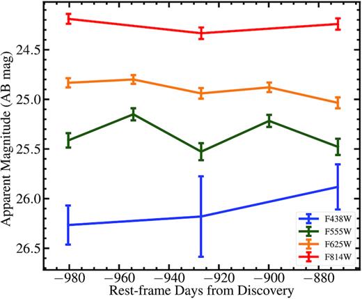
The pre-explosion light curve of the SN 2019yvr progenitor candidate in all four HST filters for which we have imaging. The source is not significantly variable, with at most 0.47 mag peak-to-peak variations as discussed in Section 4.3.
Thus, we are confident that the average photometry across all four HST bands in which we detect the progenitor candidate is representative of its overall spectral energy distribution (SED). Taking an inverse-variance weighted average of across all epochs in each band, we derive average photometry mF438W = 26.138 ± 0.162, mF555W = 25.351 ± 0.032, mF625W = 24.897 ± 0.022 mag, and mF814W = 24.253 ± 0.032 mag as shown in Table 2. Temporarily, ignoring any correction due to host extinction but accounting for Milky Way extinction, the source has mF555W − mF814W (roughly V − I) of 1.065 ± 0.045 mag and MF555W = −5.5 mag assuming our preferred distance modulus above (both values are in AB mag). This is roughly consistent with temperatures of Teff = 3360 K, which is broadly comparable, although slightly hotter, than most terminal RSGs at solar metallicity (Choi et al. 2016). This suggests that the source either has a cool photosphere or is heavily extinguished, in agreement with expectations from our analysis of SN 2019yvr. However, if the source is extinguished due to CSM, there is no clear evidence from pre-explosion variability whether any of this material was ejected during the window of the HST or Spitzer observations.
4.4 Comparison to blackbodies and single-star spectral energy distributions
Assuming that the counterpart is dominated by the SED of a single star, we estimate the luminosity and temperature of that star by fitting various SED models to the HST photometry. Broadly, we use blackbody and stellar SEDs obtained from Pickles & Depagne (2010).
We use a full forward modelling and Monte Carlo Markov Chain (MCMC) approach to simulate the in-band apparent magnitudes assuming the distance above and drawing extinction (AV) and reddening (RV) parameters following the |$\chi ^{2}_{\mathrm{ext}}$| probability distribution from our light-curve analysis in Section 3 and as shown in Fig. 5. For a blackbody with a given effective temperature Teff and luminosity L as well as extinction values drawn from the χ2 distribution discussed above, we simulate an intrinsic, absolute magnitude Mi in each band i and convert to an apparent magnitude mi with in-band Milky Way extinction AMW,i, the implied host extinction AH,i, and our preferred distance modulus μ = 30.8 mag. We include the distance modulus uncertainty in the uncertainty for our derived luminosity, but we do not incorporate this value in our MCMC as distance only affects the overall scaling of the spectral fit rather than the SED shape.
In this way, we incorporate the differences between the observed and forward-modelled magnitudes as well as between the values of AV and RV for each trial and the best-fitting values from our colour curve template fitting. Assuming a blackbody SED, we estimate the best-fitting parameters |$T_{\mathrm{eff}} = 7700\substack{+900\\-1000}$| K and |$\log (L/L_{\odot })= 5.3\substack{+0.2\\-0.3}$|. Although we include the distance modulus uncertainty in our luminosity (and radius) uncertainty estimates, we did not include this value in our fitting method as it does not affect the overall shape of the SED. The implied photospheric radius for the best-fitting blackbodies are R = 250 ± 30 R⊙. As we incorporate AV and RV from the light-curve analysis into our models, we also constrain these parameters with best-fitting values |$A_{V}=2.8\substack{+0.3\\-0.4}$| mag and |$R_{V}=5.2\substack{+0.8\\-0.7}$| assuming the intrinsic blackbody spectrum.
We also compared our photometry to single-star SEDs from Pickles & Depagne (2010). We use stars of all spectral classes, fitting only to a scaled version of the stellar SED as a function of effective temperature. Using the same MCMC method, our walkers drew a temperature randomly and then chose the stellar SED with the closest effective temperature. The best-fitting SEDs are consistent with stars in the F4–F0 range (intrinsic |$T_{\mathrm{eff}} = 6800\substack{+400\\-200}$| K; see Figs 7 and 8) with an implied luminosity log (L/L⊙) = 5.3 ± 0.2 and a photospheric radius |$R = 320\substack{+30\\-50}$| R⊙. Thus, the best-fitting values are broadly consistent between blackbody and Pickles & Depagne (2010) model SEDs. There is some systematic uncertainty in the exact temperature of the latter models given the sampling of the Pickles & Depagne (2010) spectra, which are increasingly sparse for hotter stars. However, this effect is small at temperatures 5000–10 000 K where there are 40 spectra of varying spectral classes.
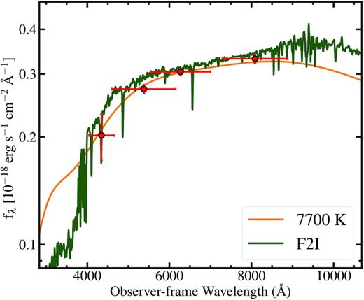
The best-fitting SEDs to the average pre-explosion HST photometry of the SN 2019yvr progenitor candidate. Our best-fitting blackbody has Teff = 7700 K, while the best-fitting single-star Pickles & Depagne (2010) model is an F2I star with Teff = 6800 K. In both cases, the implied luminosity is consistent with being log (L/L⊙) ≈ 5.3. The SEDs are completely forward modelled in observed flux, thus they include the apparent best-fitting interstellar host and Milky Way extinction. Although we include the distance uncertainty in our luminosity estimate, the error bars in this figure only include measurement uncertainty and uncertainty on extinction. We simply scale the integrated flux density by our preferred distance.
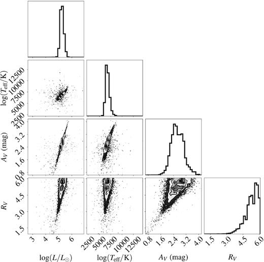
Corner plot showing the correlation between our fit parameters log (L/L⊙)and log (T/K) of a single star following a Pickles & Depagne (2010) as well as host extinction AV and host reddening RV as described in Section 4.4. The contours show the 1σ, 2σ, and 3σ best-fitting values derived from all of our samples. Although the luminosity and V-band host extinction are highly correlated, the resulting luminosity and temperature are tightly constrained.
Our treatment of AV and RV is identical to the forward modelling approach for the blackbodies above, and we derive best-fitting values of |$A_{V}=3.1\substack{+0.3\\-0.2}$| mag and |$R_{V}=5.9\substack{+0.1\\-0.4}$|. In both the blackbody and stellar SED models, our luminosity estimates are on the high-luminosity end for observed core-collapse SN progenitor stars (e.g. in Smartt et al. 2015) but consistent with most of the SN IIb progenitor stars (see Fig. 9).
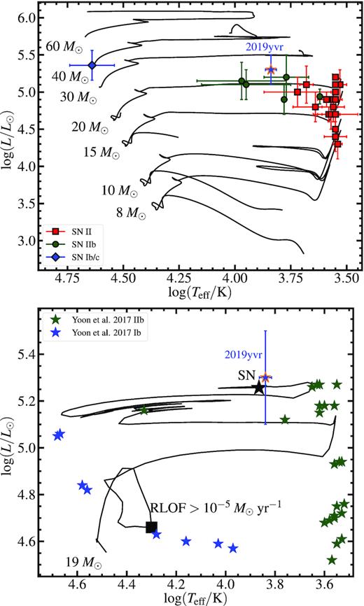
(Top): A Hertzpsrung–Russell diagram showing the location of the SN 2019yvr progenitor candidate (blue star) with comparison to SN IIb progenitor stars (green squares), iPTF13bvn (blue diamond; Cao et al. 2013; Bersten et al. 2014; Folatelli et al. 2016), and SN II progenitor stars (red squares; Smartt et al. 2015). We overplot MIST single-star evolutionary tracks from Choi et al. (2016) and Choi, Conroy & Byler (2017) for comparison. Bottom: A 19+1.9 M⊙ binary star evolution track from bpass v2.2 (Eldridge et al. 2017), which is consistent with the pre-explosion photometry of the SN 2019yvr progenitor candidate. We highlight the location on the track where the primary star begins Roche lobe overflow (RLOF; square), reaches its minimum hydrogen envelope mass (0.047 M⊙, circle), and terminates as a supernova (star). We also show binary star models from Yoon (2017) with outcomes predicted for type Ib (blue) and IIb SNe (green).
As a further check on the effect of extinction on our derived parameters, we show the relationship between the host extinction AV and reddening law parameter RV and the implied temperature and luminosity for the Pickles & Depagne (2010) models in Fig. 8. Luminosity is highly correlated with variations in AV, with AV < 2.4 mag implying a lower luminosity but also a significantly cooler photospheric temperature. In general, such a cool photosphere is associated with a massive hydrogen envelope, which is in tension with the SN Ib spectroscopic class (see Section 5 for further discussion). In contrast, a larger extinction value would imply a significantly higher luminosity and hotter temperature, although no combination of parameters we considered for the stellar SED fits allowed an effective temperature >10 000 K to within the 3σ level. This is in stark contrast with the progenitor of iPTF13bvn with Teff ≈ 45 000 K (Cao et al. 2013; Bersten et al. 2014; Eldridge & Maund 2016; Folatelli et al. 2016) and He stars generally, which tend to have effective temperatures >20 000 K (as discussed for the progenitors of SNe Ib in Yoon 2015).
Overall, our constraints on AV and RV enable a relatively tight fit temperature and luminosity as demonstrated in Fig. 8. The minimum χ2/degrees of freedom = 1.5, which suggests that a single, extinguished star is well matched to our data and we cannot effectively constrain scenarios with more free parameters, such as the inclusion of another star to the overall SED. However, while this analysis might accurately reflect the SN 2019yvr progenitor star’s evolutionary state at 2.6 yr before explosion, it does not place any specific constraints on the pathway that led to this configuration. We further explore the implications of an SN Ib progenitor star with these properties and the implications for a single-star origin in Section 5.1.
4.5 Comparison to binary star models
We also compare the SED of the SN 2019yvr progenitor candidate to binary stellar evolution tracks from BPASS (Eldridge et al. 2017), comprising 12 663 binary star models at a single metallicity. BPASS provides physical parameters from the binary star system throughout its evolutionary sequence as well as in-band absolute magnitudes for the individual components and binary system as a whole. Our analysis involved a direct comparison between the F438W, F555W, F625W, and F814W magnitudes of the SN 2019yvr counterpart and the total binary emission estimated via BPASS synthetic magnitudes in F435W, F555W, SDSS r, and F814W, respectively. As BPASS magnitudes are provided in Vega mag, we transformed our AB mag photometry to Vega mag using the relative Vega mag − AB mag zero-points for all four WFC3/UVIS filters (0.15, 0.03, −0.15, and −0.42 mag, as in Dressel 2012).
Assuming that the SN 2019yvr progenitor is one component of a binary system, we determined what BPASS evolutionary tracks have a terminal state consistent with the SN 2019yvr candidate photometry. Based on the gas-phase metallicity estimate of NGC 4666 in Pan et al. (2020), which is consistent with Solar metallicity, we restrict our analysis to BPASS models with fractional metallicity Z = 0.014. However, we emphasize that the Pan et al. (2020) metallicity estimate is derived from spectra obtained towards the centre of NGC 4666 rather than at the site of SN 2019yvr, and so the true metallicity of the SN 2019yvr progenitor system may be significantly different. Otherwise, we consider evolutionary tracks for all BPASS initial masses (Minit = 0.1–300 M⊙), mass ratios (q = 0.1–1.0), and binary periods (log (P/1 d) = 0–4).
We used the same MCMC method as above with walkers drawing from initial masses, mass ratios, and periods and comparing the terminal absolute magnitude and colours of the closest model in parameter space to the SN 2019yvr counterpart photometry. We also included AV and RV as free parameters, but with the walkers drawing from the same χ2 distribution for these parameters as in the blackbody and stellar SED fits above. For our BPASS fits, the best-fitting models correspond to initial mass Minit = 19 ± 1 M⊙, initial mass ratio q = 0.15 ± 0.05 and initial period log (P/1 d) = 0.5 ± 0.2. The small error bars on the BPASS initial binary parameters derive from the fact that few BPASS models lie within 1σ from our best-fitting model (12 out of 12 663), and so they do not reflect the full range of systematic uncertainties in binary star models used in our fitting method. We show our a Hertzpsrung–Russell diagram with the best-fitting model (Minit = 19, q = 0.1, and log (P/1 d) = 0.6) in Fig. 9 and the luminosity and temperature derived from our Pickles & Depagne (2010) stellar SED fits.
We performed our fits by comparing the observed photometry of the SN 2019yvr progenitor candidate to the apparent magnitudes inferred for the combined flux of both stars in the BPASS models,11 and so we are sensitive to scenarios where the flux from either the primary or companion star dominates the total emission. In all of the best-fitting models and all four bands we consider, the counterpart is dominated by emission from an ≈19 M⊙ primary star and the companion contributes very little to the overall flux. We found no other binary scenarios where the total flux was consistent with our photometry at the time one of the stars terminated, including scenarios where the secondary star produced the SN explosion instead (i.e. in a neutron star or black hole binary).
In the best-fitting model, the terminal state of the SN progenitor is log (L/L⊙) = 5.3 and Teff = 7300 K with a terminal mass of Mfinal = 7.3 M⊙, implying a consistent luminosity but a slightly warmer temperature than we derive from the Pickles & Depagne (2010) models. Similar to above, there are no models at the <3σ level where the exploding star has a terminal temperature >11 000 K. In the best-fitting model, the secondary star (with an initial mass of 1.9 M⊙) is mostly unchanged with only 0.009 M⊙ of material accreted by the time the primary reaches core collapse, implying that most of the mass transfer in this model was non-conservative. In addition, the BPASS models predict that 0.047 M⊙ (0.6 per cent mass fraction) of hydrogen remains in the primary in its terminal state and no model with <0.038 M⊙ is consistent with our HST photometry at the 3σ level. The best-fitting extinction values for this BPASS model was AV = 2.6 ± 0.3 mag and |$R_{V}=5.1\substack{+0.9\\-2.1}$|.
The primary effect of the BPASS evolutionary models compared to single-star models is the inclusion of Roche lobe overflow (RLOF). For our specific best-fitting model, RLOF turns on in the post-main-sequence phase (i.e. Case B mass transfer; shown with a square in Fig. 9), and continues through the end of the primary star’s evolution. In particular, mass-loss due to RLOF follows the prescription for common-envelope evolution (CEE) as the radius of the primary star is smaller than the binary separation throughout post-main sequence evolution (following prescription in Eldridge et al. 2017). The binary separation is only 8.6 R⊙ starting in the post-main sequence and at the onset of CEE, and so the primary mass-loss rate increases significantly to 1–5 × 10⁻⁴ M⊙ yr−1. This common envelope mass-loss phase largely determines the final mass and state of the primary star as it is larger than wind-driven mass-loss by a factor of ≈1000.
In BPASS, the onset of CEE is highly correlated with small binary separations and low-mass ratios for stars with Minit > 5 M⊙ (Eldridge et al. 2017). Thus stars that terminate near the progenitor candidate in the Hertzsprung–Russell diagram require a specific mass-loss scenario where CEE can strip most of the hydrogen envelope but leave a small amount (at least 0.038 M⊙ according to our models), leading to relatively tight constraints on binary mass ratio and period for our BPASS fits. However, these parameters are subject to significant systematic uncertainty in terms of the CEE and mass-loss prescriptions assumed. In Section 5.1, we discuss whether these best-fitting binary models to the pre-explosion photometry of SN 2019yvr are consistent with its classification as a type Ib SN.
5 WHAT PROGENITOR SYSTEMS COULD EXPLAIN SN 2019YVR AND THE PRE-EXPLOSION COUNTERPART?
Given our analysis in Section 4, we assume throughout this discussion that the SN 2019yvr pre-explosion counterpart is dominated by emission from the SN progenitor system. From our inferences about this source above as well as our knowledge of SN 2019yvr, we consider what evolutionary pathways could lead to the source observed in the HST photometry as well as the resulting SN. These pathways need to explain several facts referenced throughout the previous analysis, which we summarize here as follows:
SN 2019yvr was an SN Ib with no evidence for hydrogen in its early-time spectra, starting from 7 d before peak light (Dimitriadis et al. 2019) until well after peak light. Following models in Dessart et al. (2012), this suggests that the progenitor star must have had <10−3 M⊙ (but possibly as much as 0.03 M⊙; Hachinger et al. 2012) of hydrogen remaining in its envelope at the time of explosion.
SN 2019yvr began interacting with CSM starting around 150 d after explosion and exhibited strong H α, radio, and X-ray emission consistent with a shock formed in hydrogen-rich material (Auchettl et al., in preparation). Using conservative assumptions about the SN shock velocity (10 000 km s−1) and velocity of the CSM (100 km s−1), we infer that this material must have been ejected at least ≈44 yr prior to core collapse and implying a shell or clump of material at >1000 au from the progenitor system (see estimate from equation 4 in Section 5.2). Although, we find it more likely that this material came from the SN progenitor star itself given the frequency of SNe Ib with late-time interactions (i.e. similar to SN 2014C; Milisavljevic et al. 2015; Margutti et al. 2017), it is possible that this material came from a binary companion and the actual SN 2019yvr progenitor star was hydrogen free on this time-scale. Beyond this interaction, there is no evidence for dense CSM in early-time spectra or light curves, all of which appear similar to SNe Ib without evidence for these interactions.
SN 2019yvr exhibited a large line-of-sight extinction (AV ≈ 2.4 mag) while its Milky Way reddening was only E(B − V) = 0.02 mag. We infer from the strong Na i D line at the redshift of the SN 2019yvr host galaxy NGC 4666 that this extinction implies a significant dust column in the NGC 4666 interstellar medium towards SN 2019yvr and/or a correspondingly large column of circumstellar dust in the environment of the progenitor system itself. There is no clear evidence for any mass ejections or warm circumstellar gas in a compact shell around the progenitor system, either in pre-explosion data or from circumstellar interaction once SN 2019yvr exploded.
There is a single, point-like progenitor candidate to SN 2019yvr detected in pre-explosion HST imaging. This source exhibits very little photometric variability over a 110-d period from 2.7 to 2.4 yr prior to core collapse. Before applying our host extinction estimate but applying Milky Way extinction, this progenitor candidate has a red colour of mF555W − mF814W = 1.065 mag. Accounting for the inferred extinction and distance modulus above, the source is relatively luminous with MF555W = −7.8 mag (roughly in V band). This value is consistent with massive stars but low for a stellar cluster (as in Gieles et al. 2006).
Accounting for all extinction, the progenitor candidate is consistent with a log (L/L⊙) = 5.3 ± 0.2 and Teff ≈ 6800 K star, which implies a photosphere with a radius of ≈320 R⊙ at 2.6 yr prior to the SN 2019yvr explosion. Such a star would be closest in temperature and luminosity to yellow supergiants confirmed as SN IIb progenitor stars (Fig. 9 and green circles for SNe 1993J, 2008ax, 2011dh, 2013df, and 2016gkg). Comparing to stellar SEDs, the spectral type and luminosity class are best matched to F4–F0 supergiant stars.
Comparing the pre-explosion photometry to BPASS binary stellar evolution tracks in Eldridge et al. (2017), the best-fitting model is a 19 M⊙ + 1.9 M⊙ system that undergoes common envelope evolution and strips most of the material from the progenitor star. Immediately prior to explosion, the primary star retains 0.047 M⊙ of hydrogen in its envelope, inconsistent with the masses for SN Ib systems given above. No other BPASS models were consistent with both our pre-explosion photometry and a system that produced an SN explosion.
5.1 The anomalously cool progenitor and the Type Ib classification of SN 2019yvr
We compare the SN 2019yvr progenitor candidate in a Hertzsprung–Russell diagram to other known progenitor systems in Fig. 9, including SNe II (Smartt et al. 2015, and references therein), SNe IIb (SNe 1993J, 2008ax, 2011dh, 2013df, and 2016gkg; Aldering et al. 1994; Crockett et al. 2008; Maund et al. 2011; Van Dyk et al. 2014; Kilpatrick et al. 2017), and the progenitor of the SN Ib iPTF13bvn (Cao et al. 2013; Bersten et al. 2014; Folatelli et al. 2016). We also note that there is a single SN Ic progenitor candidate for SN 2017ein (Kilpatrick et al. 2018b; Van Dyk et al. 2018), but the source has a luminosity log (L/L⊙) ≈ 6.0 and temperature Teff > 105 K and so is off our plotting range (and may actually be a very young open cluster). For comparison, we also overplot single-star evolutionary tracks from the Mesa Isochrones and Stellar Tracks code (Choi et al. 2016, 2017).
The most notable feature of the SN 2019yvr progenitor candidate in Fig. 9 and compared with other stripped-envelope SN progenitor stars is its relatively cool effective temperature, which in turn implies an extended photosphere given our constraints on its SED. Assuming a single-star origin and judging solely by the source’s inferred luminosity and temperature of log (L/L⊙) = 5.3 and Teff = 6800 K, the counterpart is consistent with a 30 M⊙ star in the so-called ‘Hertzsprung gap’ (see e.g. de Jager & Nieuwenhuijzen 1997; Stothers & Chin 2001). This is in sharp contrast to the predicted progenitors of SNe Ib, which are thought to have low-mass, compact envelopes, consistent with a star that has almost no hydrogen in its outer layers (Yoon 2015).
Given these facts, we consider the implications of different progenitor scenarios. In particular, we emphasize the apparent contradiction between an SN from a star without a significant hydrogen envelope mass and a pre-explosion counterpart consistent with a massive star with a significantly extended photosphere, which typically requires a non-negligible hydrogen envelope mass. Combined with the SN 2014C-like circumstellar interaction observed at late times, SN 2019yvr may offer significant insight into mass-loss in late-stage stellar evolution for stripped-envelope SNe. Here, we review ‘standard’ single and binary star scenarios and assess whether they can explain all of these properties.
5.1.1 Single-star models
It is still debated if single massive stars can evolve to the point where they would explode as yellow supergiants, in part because the Hertzsprung gap is typically a short-lived and transitional phase in the post-main sequence. Standard single-star evolution would suggest that a star with an effective temperature of Teff = 6800 K and log (L/L⊙) = 5.3 retains a massive hydrogen envelope: a 30 M⊙ initial mass star would retain a |$60{{\ \rm per\ cent}}$| surface hydrogen mass fraction on its first passage through the Hertzsprung gap (following the structure of model stars in Choi et al. 2016). Thus, in the context of stripped-envelope SNe, any single-star model would likely enter the yellow supergiant phase after evolving through the RSG branch and shedding the remainder of its hydrogen envelope. Georgy (2012) demonstrates that such evolution is possible if RSG mass-loss rates are increased by approximately an order of magnitude towards the end of their nuclear lives.
While the physics of an enhanced late-stage mass-loss is unclear (see e.g. Yoon & Cantiello 2010), there do exist a number of luminous yellow supergiants (termed ‘yellow hypergiants’) which are hypothesized to be such post-RSG stars. Many yellow hypergiants are extremely variable with high mass-loss rates, such as ρ Cas (Smith 2014; Lobel et al. 2015) and V509 Cas (Percy & Zsoldos 1992), and are located towards the end of the luminous blue variable (LBV) bistability track (Smith, Vink & de Koter 2004). This variability involves a rapid (years to decades) evolution between quiescent, hot phases, and erupting, cool phases with extreme mass-loss episodes (e.g. 10−4 M⊙ yr−1 as in the yellow hypergiants ρ Cas and HR 8752; de Jager 1998; Humphreys, Davidson & Smith 2002).
Yellow hypergiants undergoing extreme mass-loss have been proposed as candidates for type Ib/c progenitors as their LBV-like mass ejections provide an efficient way to rid the star of its hydrogen and helium envelope in the years before core collapse (as in SN 2006jc; Foley et al. 2007; Smith & Conti 2008). The presence of these stars in the gap and the fact that some of them explode as type IIb SNe (the bluest SN IIb progenitor stars span this gap, e.g. Crockett et al. 2008; Kilpatrick et al. 2017) strengthens the association between extreme mass-loss and stripped-envelope SNe (de Jager 1998; Stothers & Chin 1999). While it is debated if such enhanced mass-loss rates are possible for single stars on the RSG branch (e.g. Beasor et al. 2020), mass-loss episodes and variability of stars near this point on the Hertzpsrung–Russell diagram suggests it is possible to rapidly shed their hydrogen envelopes and increase in temperature over time-scales of years (as observed with HR 8752, e.g. de Jager & Nieuwenhuijzen 1997). However, yellow hypergiants that we observe in this region of the Hertzsprung–Russell diagram have massive, hydrogen-rich envelopes, and their winds are known to be hydrogen rich (Smith et al. 2004). Assuming such a star exploded as a SN Ib only 2.6 yr after being observed in this evolutionary phase, it would either need to shed its remaining envelope in the final 2.6 yr or remain cool after retaining only a trace hydrogen envelope. The former scenario will be discussed in Section 5.2, below.
Alternatively, it is worth considering if a single star with virtually no remaining hydrogen in its envelope could inflate to a radius of 320 R⊙ while exhibiting a photospheric temperature of 6800 K – as required for SN 2019yvr and its progenitor candidate. The coolest known helium stars are only ≈10 000 K and these examples are significantly less luminous than the observed counterpart. For example, LSS 4300 is Teff = 11 000 K (Drilling, Landolt & Schonberner 1984; Schoenberner & Drilling 1984), KS Per is 10 000 K (Woolf 1973; Drilling & Schonberner 1982), and ν Sgr is 11 800 K (Frame et al. 1995). The counterpart we observe is only this hot assuming our SED modelling is inconsistent with the true temperature at >3σ or if there is >2 mag more extinction than we assumed at 2.6 yr before explosion. Even if we assume either of these scenarios is true, the progenitor candidate would still have log (L/L⊙) ≥ 5.3, which is much more luminous than the most luminous helium stars that reach log (L/L⊙) = 4.6 (see previous references and Dudley 1992). Thus an anomalously high-mass and luminous helium star would be needed to match to SN 2019yvr, which in general is not allowed by standard single star stellar evolution models.
5.1.2 Binary star models
As shown above, the best-fitting binary systems for our SN 2019yvr pre-explosion photometry are short-period, low-mass ratio systems that undergo CEE. While such systems are expected to have complex circumstellar environments, possibly consistent with SN 2019yvr, we emphasize that all of the BPASS models terminate with final hydrogen-envelope masses of >0.038 M⊙. This is inconsistent with a classification as an SN Ib via the models of Dessart et al. (2012) and Hachinger et al. (2012). In addition, there is debate as to whether the evolution of such high-mass ratio binaries within BPASS is representative of actual stellar systems. Neugent, Levesque & Massey (2018) and Neugent et al. (2020) argue that any star that will eventually explode as a core-collapse SN evolves off the main sequence fast enough that companion stars with initial masses ≲3 M⊙ would not have enough time to complete their contraction phase and thus would still be protostars. This is not accounted for in current BPASS models, which initialize all stellar masses on the ZAMS simultaneously.
More broadly, the progenitor systems of SNe Ib are predicted to be low-mass helium stars that evolve via binary evolution. While they can expand to moderately large radii due to shell burning, they typically remain <100 R⊙ (Kleiser et al. 2018; Laplace et al. 2020). Their photospheric temperatures are thus significantly hotter than the HST photometry of the SN 2019yvr progenitor candidate implies. The latter allows at most 11 000 K as opposed to the ≈45 000 K photosphere of the progenitor star to iPTF13bvn (Eldridge & Maund 2016; Folatelli et al. 2016). Yoon (2015) predicts that the best observational counterparts to SN Ib progenitor systems are binary, stripped WR stars similar to HD 45166 (Groh, Damineli & Hillier 2008) and WR7a (Oliveira, Steiner & Cieslinski 2003), both of which have Teff > 20 000 K. Several nearby stripped-envelope SNe have been targeted with late-time imaging to look for surviving binary companions, including the SN Ic 2002ap, which constrains the presence of a main-sequence companion star >8–10 M⊙ (Zapartas et al. 2017). The SN IIb 2001ig had a surviving companion star detected in the ultraviolet, indicating that it is a B-type main-sequence star likely with an initial mass of ≈9 M⊙ (Ryder et al. 2018).
Nearly all of these stars are (or were) thought to be in binaries with close (<few day) orbits where the primary has been stripped to 3–10 M⊙, likely through Case B mass transfer (Yoon et al. 2012; Yoon 2015, 2017). The companion can span a wide range of luminosities and evolutionary states (e.g. WR7a exhibits a 0.204 d binary orbital period, but no secondary is observed implying a very low mass star or a compact object; Pereira, Landaberry & da Conceição 1998; Oliveira et al. 2003). The primary stars are left completely stripped of a hydrogen envelope. This is in contrast to the best-fitting BPASS model, which undergoes extreme mass-loss due to CEE and RLOF during the post-main sequence but stops before the hydrogen envelope is completely depleted (Delgado & Thomas 1981; Ivanova et al. 2013; Eldridge et al. 2017).
Thus, as with the single star models, there remains significant tension as to whether any standard binary evolution model can reproduce both the progenitor candidate and a system that explodes as an SN Ib. We are left needing to invoke some additional mechanism that can account for both the cool photospheric temperature 2.6 yr prior to explosion and the negligible hydrogen envelope mass at the time of core collapse. In the following sections, we discuss two potential resolutions to this paradox (Sections 5.2 and 5.3) and highlight some evolutionary scenarios that may be allowed while also explaining the dense CSM shell observed around SN 2019yvr (Section 5.4).
5.2 Ejection of the final hydrogen envelope in the last 2.6 yr prior to core collapse
One way to resolve the apparent conflict between the extended progenitor radius and lack of hydrogen in the ejecta of SN 2019yvr would be if the progenitor star did possess a envelope with ∼0.01–0.03 M⊙ of hydrogen (similar to the yellow supergiant progenitor stars of SNe IIb) at the time of the HST observations, but somehow managed to lose this material in the intervening 2.6 yr. Such a scenario is not unprecedented: episodic mass ejections have been invoked to explain stripped-envelope SN progenitor systems that exhibit dense shells or clumps of CSM (see e.g. Chugai & Chevalier 2006; Bietenholz et al. 2014; Chandra 2018; Mauerhan et al. 2018; Pooley et al. 2019; Sollerman et al. 2020; Tartaglia et al. 2020). This was also observed directly for SN 2006jc, an SN Ib with a pre-explosion outburst 2 yr before explosion (Foley et al. 2007; Pastorello et al. 2008; Smith & Conti 2008; Maund et al. 2016), which later manifested as circumstellar interaction. Indeed, SN 2019yvr shows evidence for relatively narrow H α, radio, and X-ray emission ≈150 d after core collapse, providing evidence for episodic mass ejections throughout the progenitor’s final evolutionary stages.
Therefore, if the hydrogen we observe in CSM is the same material inferred from the progenitor star photosphere, the wind velocity must be at least 1800 km s−1 such that the progenitor star could eject it after the HST data were obtained. A wind at this speed can only be achieved by a compact and massive WR-like star (similar to those presented in Rochowicz & Niedzielski 1995; van der Hucht 2001), inconsistent with our pre-explosion photometry. Such a high velocity would therefore require and ejection mechanism capable of accelerating material to ≳10× the stellar escape speed. This would be in contrast to current theoretical models for both wave-driven mass-loss in hydrogen-poor stars (which have terminal velocities of a few hundred km s−1 Fuller & Ro 2018) and common-envelope ejections (which tend to proceed at roughly the escape velocity).
Unless a stronger ejection mechanism can be identified, while the mass-loss event that led to the material at ≈1000 au was timed soon before the explosion of SN 2019yvr, it may not be directly associated with the relatively cool photosphere we infer from the HST imaging. Multiple eruptive mass-loss events would be needed to explain both the CSM and the final depletion of the progenitor star’s hydrogen envelope assuming the pre-explosion counterpart, the source of the material around SN 2019yvr, and the SN 2019yvr progenitor star are all the same. The second ejection would place material closer to the progenitor star, which is not detected in our light curves or spectra (e.g. via enhanced emission due to CSM interaction or flash ionization features similar to Gal-Yam et al. 2014). It is possible that this material was missed due to a delay between the explosion of SN 2019yvr and its discovery, and detailed analysis of these data will be carried out in Auchettl et al. (in preparation) to assess whether or not this could be the case.
5.3 A quasi-photosphere seen as an inflated star
If the scenario discussed in Section 5.2 is not viable, then the SN 2019yvr progenitor candidate must have contained virtually no hydrogen 2.6 yr before explosion (<10−2 M⊙ as required for a type Ib classification by Dessart et al. 2012; Hachinger et al. 2012). In this case, we would require that the envelope was inflated by some process not accounted for in standard models of stellar evolution. Here, we consider two scenarios in which a star with only a trace hydrogen envelope could exhibit a photospheric radius of ≈320 R⊙ or roughly 1.5 au: (a) formation of a pseudo-photosphere in a dense stellar wind, and (b) inflation due to an additional heat/energy source that produces a radiation pressure supported envelope.
5.3.1 A stellar wind
To estimate mass-loss rate required to explain the photosphere observed for the progenitor candidate of SN 2019yvr, we assume that the wind could be as fast as 100 km s−1, as described in Section 5.2 [a detailed analysis of the CSM properties will be presented in Auchettl et al. (in preparation)]. We also use our constraint on the effective temperature of the observed photosphere Teff = 6800 K and radius R = 320 R⊙ above, which gives a local sound speed cs ≈ 7 km s−1 and implies |$\dot{M}\gt 1.3\times 10^{-4}~\mathrm{M}_{\odot }~\mathrm{yr}^{-1}$|.
This mass-loss rate is extreme for a star with log (L/L⊙) = 5.3 (even yellow hypergiants or low-luminosity LBVs as in Smith et al. 2004), which tend to have time-averaged |$\dot{M}\approx 10^{-5}~\mathrm{M}_{\odot }~\mathrm{yr}^{-1}$| (Humphreys & Davidson 1994). However, the total mass of material needed to form a quasi-photosphere is only |$\dot{M} v_{\mathrm{ w}}^{-1} R_{\tau } \approx 10^{-5}~\mathrm{M}_{\odot}$|. This material can easily be shed from the star’s remaining hydrogen/helium envelope over a brief period of strong mass-loss, although the time-scale for such a shell to form would be only Rτ/v|$\mathrm{ w}$| = 26 d.
However, we do not observe any emission lines or ‘flash spectroscopy’ features in our early spectra of SN 2019yvr as may be expected if dense wind material is present. This scenario would also require a significant change in the mass-loss from the SN 2019yvr progenitor timed ≲3 yr prior to explosion, which is closely aligned with predictions for instabilities during oxygen burning (Meakin & Arnett 2006; Arnett, Meakin & Viallet 2014). However, there is no other evidence for a dense wind that could form the observed photosphere.
5.3.2 A radiation dominated envelope
However, even in this case several mysteries remain as to the nature of the progenitor system. In particular, for a complete description of SN 2019yvr, the progenitor system would still need to eject a shell of hydrogen-rich material at ∼1000 au. This will be be discussed in Section 5.4.
5.4 Progenitor scenarios for SN 2019yvr
In the sections above, we have argued that reconciling the extended progenitor radius and lack of hydrogen in the ejecta of SN2019yvr requires a system that either:
ejected the remainder of its hydrogen envelope in the final 2.6 yr pre-explosion (Section 5.2).
undergoes a process not accounted for in standard models of evolution and that leads to additional inflation or has sufficient material around the progenitor to form a quasi-photosphere in the CSM (Section 5.3).
In addition, in either case, a viable progenitor scenario for SN 2019yvr must also explain a shell of hydrogen-rich material observed at ∼1000 au that was likely ejected 50–100 yr prior to explosion. Below we consider two pathways that may be consistent within these constraints. We emphasize that this is not an exclusive list of possible scenarios. No existing model currently explains all the observed properties of SN 2019yvr and its progenitor system.
5.4.1 A luminous blue variable phase
One evolutionary pathway that naturally explains many of the observables for SN 2019yvr is a series of eruptions from a massive star in an LBV phase. These eruptions are known to precede many SNe, some of which are thought to be core-collapse explosions (as was argued for SN 2009ip Mauerhan et al. 2013), although this interpretation of LBVs as a phase immediately preceding core collapse remains controversial (Margutti et al. 2014).
Many types of progenitor systems exhibit pre-SN eruptions in the final years to weeks before explosion, notably for the progenitors of SNe IIn (SNe with narrow Balmer lines in their optical spectra, indicative of interaction between ejecta and a dense mass of CSM; Smith 2017). These systems must eject from 0.1–10 M⊙ over short time-scales (Smith & McCray 2007; Fox et al. 2010, 2011) requiring an extreme mass-loss rate and variability on the time-scale of the eruptions. Their progenitor systems have also been observed in the literature, notably for SN 2009ip whose progenitor star had an initial mass >60 M⊙ (Smith et al. 2009; Foley et al. 2011). Although there is some ambiguity whether these events are actually terminal explosions of massive stars (Mauerhan et al. 2013; Margutti et al. 2014), the eruptive mechanism that fills their environments with dense shells of CSM may be more common among stars at a wide range of initial masses. Indeed, so-called SN impostors (lower luminosity, likely non-terminal explosions of massive stars that resemble SNe IIn; Van Dyk et al. 2000; Maund et al. 2006; Pastorello et al. 2010; Ofek et al. 2016) come from systems with initial masses possibly as low as 20 M⊙ (Kilpatrick et al. 2018a). Such an eruption for SN 2019yvr and SN 2014C-like events (hypothesized by Milisavljevic et al. 2015) could explain the source of the CSM, although most SN IIn and SN impostor progenitor stars retain some hydrogen leading to broad Balmer lines in their spectra.
For SN 2019yvr, we would require a scenario analogous to SNe IIn and Ibn with strong circumstellar interaction soon after explosion (Hosseinzadeh et al. 2017; Smith 2017) but involving multiple mass-loss episodes timed years or even decades ahead of core collapse instead of months to years. The main caveat in invoking this progenitor scenario is whether episodic mass ejections can fully strip the progenitor star’s hydrogen envelope on the time-scale required by our HST observations. While LBV eruptions provide a compelling mass-loss scenario as progenitor systems extend nearly to the parameter space of the Hertzsprung-Russell diagram where we find the SN 2019yvr counterpart (see SN 2009ip, 2015bh, Gaia16cfr; Smith et al. 2009; Mauerhan et al. 2013; Elias-Rosa et al. 2016; Thöne et al. 2017; Kilpatrick et al. 2018a), these events tend to result in hydrogen-rich explosions with long-lived Balmer emission. The final eruptions of SN 2019yvr would need to strip a sufficiently small amount of hydrogen (potentially hundredths of a Solar mass as in Section 4.5) that interaction with this material would not be observed in early-time spectra. Detailed analysis of the initial observations of SN 2019yvr could place stronger constraints on whether this scenario occurred.
5.4.2 A common envelope mass-loss scenario
An alternative evolutionary pathway in the final decades of evolution for the SN 2019yvr, and put forward for SN 2014C in Margutti et al. (2017), is CEE leading to ejection of the primary star’s hydrogen envelope <100 yr before explosion. In general, this is not expected as RLOF and CEE are commonly associated with mass transfer much earlier in the primary star’s life cycle, for example, immediately after helium core contraction as discussed in Section 1. The progenitor would need to be inflated in a later evolutionary stage after helium burning to restart mass transfer (i.e. through Case C mass transfer, see Schneider et al. 2015). This is predicted to occur for only ∼5–6 per cent of binary system with primary masses between 8−20 M⊙ (Podsiadlowski, Joss & Hsu 1992).
However, if the primary star’s envelope can inflate during this phase, the companion will spiral inward and start CEE, resulting in the ejection of a significant fraction of the envelope over <1 yr (Ivanova et al. 2013). The velocity of that material would be comparable to the escape velocity of the primary, and so would likely be <100 km s−1 depending on the envelope structure of the primary star at onset of CEE. In this way, the material could survive long enough that the SN ejecta can encounter it within the first year after core collapse, as observed at ∼150 d in SN 2019yvr.
The key question for SN 2019yvr is how the post-CEE system evolves in the final years before core collapse such that it resembles the pre-explosion counterpart and also explodes as an SN Ib. Case-C CEE is an appealing solution to this problem as the remaining envelope is predicted to become unstable, leading to dynamical pulsations and steady mass loss in the remaining years before core collapse (especially for extremely luminous stars; Heger et al. 1997). Thus a post-CEE star could still form a quasi-photosphere assuming the mass-loss rate exceeded 10−4 M⊙ yr−1 as in Section 5.3. Alternatively, the inspiral during CE phase itself supplies a source of heat in the stellar envelope. Thus, after the ejection of most of its hydrogen envelope, the resulting post-CEE hydrogen-deficient envelope could remain partly inflated. If the resulting star was dynamically unstable and losing mass significantly faster than the ≈10−5 M⊙ yr−1 predicted for yellow hypergiants (Humphreys & Davidson 1994), it could rapidly shed even the 10−2–10−1 M⊙ that is predicted to remain in the envelope of comparable stars from BPASS. This would simultaneously explain the circumstellar material as the result of CEE, the apparently cool photosphere, and the lack of hydrogen in the primary star’s envelope at core collapse.
5.5 Comparisons to progenitor star constraints for SN 2014C and SNe Ib with late-time circumstellar interaction
SNe Ib with late-time circumstellar interaction similar to SN 2019yvr are not unprecedented and may in fact represent a large fraction of stripped-envelope SNe overall. As discussed in Section 1, SN 2014C began interacting with its circumstellar environment a few weeks after explosion (Margutti et al. 2017), and both SN 2019yvr and SN 2014C have relatively deep progenitor constraints considering both have pre-explosion HST imaging and occurred at ≈15 Mpc (Milisavljevic et al. 2015). More broadly, there are numerous examples of stripped-envelope SNe with circumstellar interaction soon after explosion (Chugai & Chevalier 2006; Bietenholz et al. 2014; Chandra 2018; Mauerhan et al. 2018; Pooley et al. 2019; Sollerman et al. 2020; Tartaglia et al. 2020), and so any mechanism that we invoke above may need to explain the presence of CSM for a significant fraction of all core-collapse SNe (Margutti et al. 2017).
A compact star cluster towards the position of SN 2014C in pre-explosion imaging (Milisavljevic et al. 2015) had a best-fitting age in the range 30–300 Myr, although it could be as young as 10 Myr. This age implies a main-sequence turnoff mass of 3.5–9.5 M⊙ depending on the metallicity of the cluster. Assuming this cluster hosted the SN 2014C progenitor star and considering the fact that stars in this mass range either do not explode as core-collapse SNe or are thought to lead to SNe II, Milisavljevic et al. (2015) inferred that a more likely explosion scenario for SN 2014C was through binary star channels for a star with an LBV-like phase and MZAMS >20 M⊙ (implying that the cluster is younger than its colours suggest). Given the photometric and spectroscopic similarity between SNe 2014C and 2019yvr and the presence of a strong density gradient in the circumstellar environments of both, it is possible that both systems could be explained through eruptive, LBV-like mass-loss or CEE as discussed above.
However, these evolutionary phases would require that the SN 2019yvr progenitor star had extreme photometric variability, and the lack of any such variability in the pre-explosion photometry indicates that these episodes would have occurred outside the short window in which we constrain the progenitor star’s evolution. Assuming that the mass-loss episode was driven by an instability in late-stage nuclear burning (e.g. Arnett et al. 2014), the star could also be inflated temporarily. Smith & Arnett (2014) suggest this inflation would occur on a time-scale comparable to the orbital period in binary systems, but we see no signature of this variability on 30–100 d time-scales. Deep, high-cadence limits, such as those from the Young Supernova Experiment (Jones et al. 2019, Auchettl et al., in preparation) or the upcoming Vera C. Rubin Observatory Legacy Survey of Space and Time (down to r ≈ 24.5 mag on a 3–4 d cadence; Ivezić et al. 2019), will be able to detect or rule out these mass-loss episodes for future events, potentially constraining the progenitor scenarios for stripped-envelope SNe in the volume where such variability is detectable.
6 CONCLUSIONS
We present pre-explosion imaging, photometry, and spectroscopy of the SN Ib 2019yvr. We find:
SN 2019yvr was an SN Ib with a large line-of-sight extinction spectroscopically similar to iPTF13bvn. SN 2019yvr exhibited signatures of interaction 150 d after discovery consistent with a shock between SN ejecta and dense, hydrogen-rich CSM (Auchettl et al. in preparation) and similar to SN 2014C (Milisavljevic et al. 2015; Margutti et al. 2017). This interaction suggests that the SN 2019yvr progenitor star underwent an eruptive mass-loss episode at least 44 yr before explosion.
There is a single source in Hubble Space Telescope imaging obtained ≈2.6 yr before discovery and consistent with being the progenitor system of SN Ib 2019yvr. Comparing to blackbodies, single-star SEDs, and binary star models, we find that the SN 2019yvr progenitor star is consistent with a star with log (L/L⊙) = 5.3 ± 0.2, |$T_{\mathrm{eff}} = 6800\substack{+400\\-200}$| K, and thus close (<5 d period) binary-star models with initial masses around 19 M⊙. However, the cool effective temperature and high luminosity implies a remaining hydrogen envelope mass of at least 0.047 M⊙ in the binary star model, which is inconsistent with the lack of hydrogen in spectra of SN 2019yvr.
Comparison to SN Ib progenitor candidates indicates that SN 2019yvr is much cooler than what is predicted for a hydrogen-stripped star, much more similar to the identified progenitors of type IIb SNe. Overall, the progenitor candidate appears cool and inflated relative to the progenitor of iPTF13bvn and helium stars.
We infer that an extreme and episodic mass-loss scenario is required to produce both a stripped-envelope SN progenitor system and the luminous, cool progenitor candidate. The binary evolution scenarios discussed above do not incorporate physical scenarios that can lead to extreme or eruptive mass-loss soon before explosion, and barring such a mass-loss scenario they do not produce a star whose hydrogen envelope is consistent with the SN Ib classification. We propose that LBV-like mass ejections or CEE provide natural explanations for the stellar classification, the lack of a massive hydrogen envelope, and the presence of dense CSM. We hypothesize that if this mass-loss mechanism occurs, the star could have formed a quasi-photosphere from CSM in its environment, requiring either a mass-loss at a rate >1.3 M⊙ yr−1 or a radiation supported hydrogen envelope with a mass >10−4M⊙ at 2.6 yr before core collapse.
ACKNOWLEDGEMENTS
We thank J.J. Eldridge and H. Stevance for helpful comments about our BPASS analysis, J. A. Vilchez, A. Campillay, Y. K. Riveros, and N. Ulloa for help with the Swope observations, as well as R. Carrasco for support of our Gemini-S/GSAOI programme. CDK acknowledges support through NASA grants in support of Hubble Space Telescope programmes GO-15691 and AR-16136. MRD acknowledges support from the NSERC through grant RGPIN-2019-06186, the Canada Research Chairs Program, the Canadian Institute for Advanced Research (CIFAR), and the Dunlap Institute at the University of Toronto. KA was supported by the Danish National Research Foundation (DNRF132) and VILLUM FONDEN Investigator grant (project number 16599). Parts of this research were supported by the Australian Research Council Centre of Excellence for All Sky Astrophysics in 3 Dimensions (ASTRO 3D), through project number CE170100013. DOJ was supported by a Gordon and Betty Moore Foundation postdoctoral fellowship at the University of California, Santa Cruz. Support for this work was provided by NASA through the NASA Hubble Fellowship grant HF2-51462.001 awarded by the Space Telescope Science Institute, which is operated by the Association of Universities for Research in Astronomy, Inc., for NASA, under contract NAS5-26555. The UCSC team is supported in part by NASA grant NNG17PX03C, NASA grants in support of Hubble Space Telescope programmes AR-14296 and GO-16239 through STScI, NSF grant AST-1815935, the Gordon and Betty Moore Foundation, the Heising-Simons Foundation, and by a fellowship from the David and Lucile Packard Foundation to RJF. JH was supported by a VILLUM FONDEN Investigator grant (project number 16599). WJG is supported by the National Science Foundation Graduate Research Fellowship Program under Grant No. DGE-1842165. RM acknowledges support by the National Science Foundation under Award No. AST-1909796. RM acknowledges support by the National Science Foundation under Awards No. AST-1909796 and AST-1944985. RM is a CIFAR Azrieli Global Scholar in the Gravity & the Extreme Universe Program, 2019 and a Alfred P. Sloan Fellow in Physics, 2019. The Margutti team at Northwestern is partially funded by the Heising-Simons Foundation under grant #2018-0911 (PI: Margutti). ERR is supported by the Heising-Simons Foundation, the Danish National Research Foundation (DNRF132) and NSF. Based on observations obtained at the Gemini Observatory, which is operated by the Association of Universities for Research in Astronomy, Inc., under a cooperative agreement with the NSF on behalf of the Gemini partnership: the National Science Foundation (United States), National Research Council (Canada), CONICYT (Chile), Ministerio de Ciencia, Tecnología e Innovación Productiva (Argentina), Ministério da Ciência, Tecnologia e Inovação (Brazil), and Korea Astronomy and Space Science Institute (Republic of Korea). The Gemini-S/GSAOI observations in this paper were obtained under program GS-2020A-Q-221 (PI Kilpatrick). Some of the data presented herein were obtained at the W. M. Keck Observatory, which is operated as a scientific partnership among the California Institute of Technology, the University of California, and the National Aeronautics and Space Administration. The Observatory was made possible by the generous financial support of the W. M. Keck Foundation. The authors wish to recognize and acknowledge the very significant cultural role and reverence that the summit of Maunakea has always had within the indigenous Hawaiian community. We are most fortunate to have the opportunity to conduct observations from this mountain. This work makes use of observations from the LCO network through program NOAO2019B-004 (PI Kilpatrick). Based on observations made with the NASA/ESA Hubble Space Telescope, obtained from the data archive at the Space Telescope Science Institute. STScI is operated by the Association of Universities for Research in Astronomy, Inc. under NASA contract NAS 5-26555. This work is based in part on observations made with the Spitzer Space Telescope, which was operated by the Jet Propulsion Laboratory, California Institute of Technology under a contract with NASA (AST-1911206 and AST-1852393).
Facilities: Gemini (GSAOI), HST (WFC3), Keck (LRIS), LCO (FLOYDS, Sinistro), Spitzer (IRAC), and Swope (Direct/4K×4K) .
DATA AVAILABILITY
All imaging, spectroscopy, and relevant data products presented in this article are available upon request. The Hubble Space Telescope and Spitzer Space Telescope data are publicly available and can be accessed from the Mikulski Archive for Space Telescopes (https://archive.stsci.edu/hst/) and Spitzer Heritage Archive (http://sha.ipac.caltech.edu/applications/Spitzer/SHA/), respectively.
Footnotes
SN 2019yvr is also called ATLAS19benc. We use SN 2019yvr throughout this paper for consistency with follow-up reports.
IRAF is distributed by the National Optical Astronomy Observatory, which is operated by the Association of Universities for Research in Astronomy (AURA) under a cooperative agreement with the National Science Foundation.
In our BPASS v2.2.1 fits, we examined columns 53–73, representing the absolute magnitude and colours from the combined flux of both the primary and companion star.
REFERENCES
APPENDIX A:
SN 2019yvr photometry.
| MJD (Epoch) | Filter | Magnitude (Uncertainty)a | Source |
|---|---|---|---|
| 58849.333 (−4.947) | B | 16.781 (0.012) | Swope |
| 58850.355 (−3.925) | B | 16.691 (0.011) | Swope |
| 58851.322 (−2.958) | B | 16.577 (0.013) | Swope |
| 58852.308 (−1.972) | B | 16.606 (0.014) | Swope |
| 58853.365 (−0.915) | B | 16.570 (0.014) | Swope |
| 58869.334 (15.054) | B | 17.772 (0.022) | Swope |
| 58871.311 (17.031) | B | 17.970 (0.020) | Swope |
| 58872.330 (18.050) | B | 18.053 (0.023) | Swope |
| 58874.339 (20.059) | B | 18.267 (0.047) | Swope |
| 58876.301 (22.021) | B | 18.234 (0.018) | Swope |
| 58849.331 (−4.949) | V | 15.822 (0.009) | Swope |
| 58850.354 (−3.926) | V | 15.701 (0.008) | Swope |
| 58851.321 (−2.959) | V | 15.647 (0.009) | Swope |
| 58852.307 (−1.973) | V | 15.648 (0.009) | Swope |
| 58853.364 (−0.916) | V | 15.565 (0.009) | Swope |
| 58869.332 (15.052) | V | 16.302 (0.011) | Swope |
| 58871.309 (17.029) | V | 16.440 (0.010) | Swope |
| 58872.329 (18.049) | V | 16.476 (0.011) | Swope |
| 58874.338 (20.058) | V | 16.679 (0.024) | Swope |
| 58876.298 (22.018) | V | 16.689 (0.009) | Swope |
| 58846.307 (−7.973) | g | 16.590 (0.014) | LCO |
| 58847.304 (−6.976) | g | 16.440 (0.013) | LCO |
| 58848.301 (−5.979) | g | 16.317 (0.012) | LCO |
| 58849.326 (−4.954) | g | 16.293 (0.009) | Swope |
| 58850.296 (−3.984) | g | 16.147 (0.021) | LCO |
| 58850.351 (−3.929) | g | 16.170 (0.008) | Swope |
| 58851.317 (−2.963) | g | 16.123 (0.009) | Swope |
| 58852.302 (−1.978) | g | 16.050 (0.007) | Swope |
| 58852.338 (−1.942) | g | 16.022 (0.011) | LCO |
| 58853.359 (−0.921) | g | 16.036 (0.008) | Swope |
| 58853.420 (−0.860) | g | 15.946 (0.012) | LCO |
| 58854.506 (0.226) | g | 16.011 (0.016) | LCO |
| 58855.506 (1.226) | g | 15.982 (0.010) | LCO |
| 58856.668 (2.388) | g | 15.902 (0.023) | LCO |
| 58857.672 (3.392) | g | 16.024 (0.032) | LCO |
| 58859.020 (4.740) | g | 16.130 (0.014) | LCO |
| 58861.015 (6.735) | g | 16.170 (0.026) | LCO |
| 58862.012 (7.732) | g | 16.226 (0.021) | LCO |
| 58866.340 (12.060) | g | 16.736 (0.014) | LCO |
| 58867.422 (13.142) | g | 16.817 (0.012) | LCO |
| 58869.328 (15.048) | g | 17.019 (0.011) | Swope |
| 58869.636 (15.356) | g | 16.993 (0.014) | LCO |
| 58871.304 (17.024) | g | 17.130 (0.013) | Swope |
| 58872.325 (18.045) | g | 17.204 (0.011) | Swope |
| 58872.329 (18.049) | g | 17.098 (0.015) | LCO |
| 58874.327 (20.047) | g | 17.371 (0.009) | Swope |
| 58875.307 (21.027) | g | 17.230 (0.015) | LCO |
| 58876.287 (22.007) | g | 17.447 (0.008) | Swope |
| 58876.338 (22.058) | g | 17.319 (0.015) | LCO |
| 58877.425 (23.145) | g | 17.340 (0.016) | LCO |
| 58846.309 (−7.971) | i | 15.551 (0.010) | LCO |
| 58847.306 (−6.974) | i | 15.427 (0.009) | LCO |
| 58848.303 (−5.977) | i | 15.321 (0.009) | LCO |
| 58849.300 (−4.980) | i | 15.192 (0.008) | LCO |
| 58849.325 (−4.955) | i | 15.181 (0.007) | Swope |
| 58850.298 (−3.982) | i | 15.133 (0.008) | LCO |
| 58850.350 (−3.930) | i | 15.028 (0.007) | Swope |
| 58851.316 (−2.964) | i | 14.977 (0.007) | Swope |
| 58851.340 (−2.940) | i | 15.063 (0.008) | LCO |
| 58852.301 (−1.979) | i | 14.942 (0.007) | Swope |
| 58852.340 (−1.940) | i | 15.009 (0.008) | LCO |
| 58853.358 (−0.922) | i | 14.878 (0.006) | Swope |
| 58853.422 (−0.858) | i | 14.858 (0.009) | LCO |
| 58854.508 (0.228) | i | 14.880 (0.013) | LCO |
| 58855.508 (1.228) | i | 14.839 (0.007) | LCO |
| 58856.670 (2.390) | i | 14.726 (0.013) | LCO |
| 58857.674 (3.394) | i | 14.789 (0.014) | LCO |
| 58859.023 (4.743) | i | 14.763 (0.008) | LCO |
| 58859.681 (5.401) | i | 14.726 (0.012) | LCO |
| 58861.017 (6.737) | i | 14.740 (0.013) | LCO |
| 58862.015 (7.735) | i | 14.783 (0.012) | LCO |
| 58863.012 (8.732) | i | 14.799 (0.012) | LCO |
| 58866.342 (12.062) | i | 15.077 (0.008) | LCO |
| 58867.425 (13.145) | i | 15.089 (0.008) | LCO |
| 58869.327 (15.047) | i | 15.086 (0.007) | Swope |
| 58869.639 (15.359) | i | 15.216 (0.008) | LCO |
| 58871.258 (16.978) | i | 15.265 (0.009) | LCO |
| 58871.303 (17.023) | i | 15.145 (0.007) | Swope |
| 58872.324 (18.044) | i | 15.166 (0.006) | Swope |
| 58872.332 (18.052) | i | 15.304 (0.008) | LCO |
| 58873.331 (19.051) | i | 15.353 (0.084) | LCO |
| 58874.323 (20.043) | i | 15.327 (0.054) | Swope |
| 58874.328 (20.048) | i | 15.342 (0.018) | LCO |
| 58875.309 (21.029) | i | 15.393 (0.008) | LCO |
| 58876.341 (22.061) | i | 15.473 (0.008) | LCO |
| 58877.427 (23.148) | i | 15.434 (0.008) | LCO |
| 58878.613 (24.333) | i | 15.518 (0.010) | LCO |
| 58882.099 (27.819) | i | 15.562 (0.008) | LCO |
| 58846.308 (−7.972) | r | 15.798 (0.010) | LCO |
| 58847.305 (−6.975) | r | 15.638 (0.009) | LCO |
| 58848.302 (−5.978) | r | 15.562 (0.008) | LCO |
| 58849.299 (−4.981) | r | 15.501 (0.010) | LCO |
| 58849.323 (−4.957) | r | 15.419 (0.007) | Swope |
| 58850.297 (−3.983) | r | 15.370 (0.009) | LCO |
| 58850.349 (−3.931) | r | 15.302 (0.006) | Swope |
| 58851.314 (−2.966) | r | 15.256 (0.007) | Swope |
| 58851.339 (−2.941) | r | 15.293 (0.009) | LCO |
| 58852.299 (−1.981) | r | 15.227 (0.007) | Swope |
| 58852.339 (−1.941) | r | 15.250 (0.009) | LCO |
| 58853.357 (−0.923) | r | 15.141 (0.007) | Swope |
| 58853.421 (−0.859) | r | 15.153 (0.009) | LCO |
| 58854.507 (0.227) | r | 15.174 (0.014) | LCO |
| 58855.507 (1.227) | r | 15.149 (0.008) | LCO |
| 58856.669 (2.389) | r | 15.106 (0.013) | LCO |
| 58857.673 (3.393) | r | 15.078 (0.017) | LCO |
| 58859.021 (4.741) | r | 15.119 (0.012) | LCO |
| 58859.674 (5.394) | r | 15.102 (0.013) | LCO |
| 58861.016 (6.736) | r | 15.197 (0.019) | LCO |
| 58862.014 (7.734) | r | 15.200 (0.013) | LCO |
| 58866.341 (12.061) | r | 15.567 (0.009) | LCO |
| 58867.423 (13.143) | r | 15.601 (0.008) | LCO |
| 58869.326 (15.046) | r | 15.664 (0.007) | Swope |
| 58869.638 (15.358) | r | 15.746 (0.009) | LCO |
| 58871.301 (17.021) | r | 15.748 (0.007) | Swope |
| 58872.323 (18.043) | r | 15.781 (0.007) | Swope |
| 58872.331 (18.051) | r | 15.840 (0.009) | LCO |
| 58873.329 (19.049) | r | 15.958 (0.087) | LCO |
| 58874.321 (20.041) | r | 15.893 (0.009) | Swope |
| 58875.308 (21.028) | r | 15.941 (0.008) | LCO |
| 58876.340 (22.060) | r | 16.056 (0.009) | LCO |
| 58877.426 (23.146) | r | 16.036 (0.008) | LCO |
| 58878.612 (24.332) | r | 16.078 (0.010) | LCO |
| 58849.327 (−4.953) | u | 18.413 (0.031) | Swope |
| 58850.352 (−3.928) | u | 18.454 (0.032) | Swope |
| 58850.352 (−3.928) | u | 18.455 (0.032) | Swope |
| 58851.319 (−2.961) | u | 18.569 (0.032) | Swope |
| 58852.303 (−1.977) | u | 18.622 (0.027) | Swope |
| 58853.360 (−0.920) | u | 18.743 (0.032) | Swope |
| 58869.329 (15.049) | u | 19.946 (0.186) | Swope |
| 58874.329 (20.049) | u | 20.772 (0.268) | Swope |
| 58876.290 (22.010) | u | 20.672 (0.252) | Swope |
