Correcting HIRES/Keck radial velocities for small systematic errors

ABSTRACT

The HIRES spectrograph, mounted on the 10-m Keck-I telescope, belongs to a small group of radial-velocity (RV) instruments that produce stellar RVs with long-term precision down to ∼1 m s⁻¹. In 2017, the HIRES team published 64,480 RVs of 1699 stars, collected between 1996 and 2014. In this bank of RVs, we identify a sample of RV-quiet stars, whose RV scatter is <10 m s⁻¹, and use them to reveal two small but significant nightly zero-point effects: a discontinuous jump, caused by major modifications of the instrument in August 2004, and a long-term drift. The size of the 2004 jump is 1.5 ± 0.1 m s⁻¹, and the slow zero-point variations have a typical magnitude of ≲ 1 m s⁻¹. In addition, we find a small but significant correlation between stellar RVs and the time relative to local midnight, indicative of an average intra-night drift of 0.051 ± 0.004 m s⁻¹ h⁻¹. We correct the 64 480 HIRES RVs for the systematic effects we find, and make the corrected RVs publicly available. Our findings demonstrate the importance of observing RV-quiet stars, even in the era of simultaneously-calibrated RV spectrographs. We hope that the corrected HIRES RVs will facilitate the search for new planet candidates around the observed stars.

instrumentation: spectrographs, techniques: radial velocities, planetary systems

1 INTRODUCTION

The fact that stellar radial-velocity (RV) measurements are prone to instrumental systematic errors is known for more than a century (e.g., Albrecht 1914). Over the years, it has become a common practice to observe standard RV stars to calibrate the instrumental zero-point RVs and enable inter-comparison between different instruments (see, e.g., Stefanik, Latham & Torres 1999, for historic review). Udry, Mayor & Queloz (1999) reported on regularly following a set of 50 standard stars with CORAVEL (Baranne, Mayor & Poncet 1979), and using them to correct for instrumental zero-point drifts of >1 km s⁻¹. In their pioneering work with the HF absorption cell as a simultaneous reference, Campbell, Walker & Yang (1988) achieved long-term precision of ∼13 m s⁻¹ by correcting the stellar RVs for run-to-run zero-point variations, which they measured using the non-variable stars of their survey.

The technological progress in the past three decades led to significant improvements in RV measurement precision. The advent of simultaneous calibration methods and environmentally stabilized spectrographs, enabled instruments, such as HIRES (Vogt et al. 1994) and HARPS (Mayor et al. 2003), to reach long-term precision of ∼1 m s⁻¹. ESPRESSO now promises to break the 1 m s⁻¹ limit in the coming years (e.g., Pepe, Ehrenreich & Meyer 2014). However, these instruments heavily rely on sophisticated calibration schemes, and the practice of using standard RV stars to correct for systematic errors was largely abandoned.

HIRES is a general-purpose high-resolution visible-light slit spectrograph mounted on the 10-m Keck-I telescope (Vogt et al. 1994). To enable precision RV measurements, an absorption Iodine cell was placed in front of the slit, which enabled measurement precision down to ∼3 m s⁻¹ (Butler et al. 1996; Vogt et al. 2000). In August 2004, a major upgrade of HIRES was performed, which improved the limiting RV precision by factor ∼3 (Butler et al. 2006). HIRES shares time on the Keck-I telescope with several other instruments. Therefore, observations of bright stars for precision RV measurements are typically scheduled around bright times. Over the years, HIRES was extensively used to search for exoplanets around bright dwarf stars (e.g., Vogt et al. 2002, 2005; Butler et al. 2003, 2004, 2006; Cumming et al. 2008). Although the survey included many RV-stable stars, their RVs were used mainly to monitor the long-term stability of the instrument, but not to correct for systematic zero-point variations (e.g., Vogt 2002; Vogt et al. 2015).

In this paper, we use publicly-available HIRES measurements to find and correct for small systematic RV variations. For the benefit of the exoplanet community, we upload the corrected RVs, and the code we used to calculate the correction, to dedicated websites.

2 THE PUBLIC HIRES RVS AND AUXILIARY DATA

In a legacy paper, Butler et al. (2017) published 64 480 observations of 1699 stars,¹ collected with HIRES between 1996 and 2014 as part of a long-term search for exoplanets. The vast majority of the observed stars were chromospherically-inactive F, G, K, and M dwarfs, and most of them were observed over a time baseline of three years or more.

In order to search for systematic effects in the HIRES data, we analysed the un-binned data provided by Butler et al. (2017). Each observation is described by its Barycentric Julian Date (BJD), exposure time (t_exp), median number of photons per pixel (⁠|$\overline{n_{\rm phot}}$|⁠), RV, RV uncertainty, and two indices of chromospheric activity.

Fig. 1 shows the RV standard deviation, std(RV), as a function of the number of RVs per star (n_RV) in the HIRES data. For robustness against outliers and small-number statistics, we estimated std as 1.48 times the median absolute deviation (MAD) around the median (e.g., Rousseeuw & Croux 1993). The std (RV) distribution peaks at 5–6  m s⁻¹, with tails extending down to ∼2 m s⁻¹ and up to >100 m s⁻¹. For the purpose of studying systematic RV errors, we focused only on reliable RV-quiet stars, which we defined as those with n_RV ≥ 5 and std(RV) <10 m s⁻¹. We found 797 such stars, with a total of 39 930 RVs.

Figure 1.

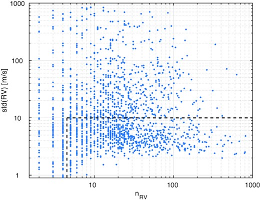
The HIRES targets published by Butler et al. (2017): std(RV) and n_RV per star. We used only the stars with n_RV ≥ 5 and std (RV) <10 m s⁻¹ in the search of systematic effects (dashed line). The Y-axis is limited to 1 km s⁻¹ as the more variable stars are irrelevant to the work presented here.

3 SMALL SYSTEMATIC ERRORS IN HIRES RVS

3.1 Nightly zero-point RV variations

We calculated an instrumental nightly zero-point RV (NZP) for each night in which at least three different RV-quiet stars were observed. The NZP of each observing night was taken as the weighted average RV of the RV-quiet stars that were observed in that night. In the 18.4 years of HIRES data provided by Butler et al. (2017), we found 913 nights for which we could calculate an NZP. For completeness, we summarize our NZP calculation method in the Appendix.

Fig. 2 shows the RVs used to calculate the NZPs, and the derived NZPs. The NZPs have a weighted rms of ∼1.20 m s⁻¹ and an effective uncertainty of 〈δNZP〉₋₂ ∼ 0.74 m s⁻¹, which gives a |$\chi ^2_{\rm red}$| of ∼2.61 (Zechmeister et al. 2013). Hence, the NZPs reveal an additional source of systematic RV scatter, on top of the internal RV uncertainties. We note that the minimum criteria for RVs to be used in calculating the NZPs were chosen after extensive optimization. More conservative criteria, such as n_RV ≥ 10, std(RV) <8 m s⁻¹, and n_RV/night ≥ 5, lead to very similar set of NZPs as presented in Fig. 2. Specifically, the typical difference between the NZPs calculated with the two different sets of criteria is twice as small as the typical NZP uncertainty.

Figure 2.

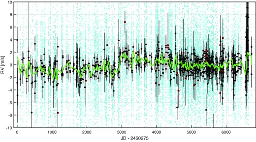
Systematic variations of the HIRES zero-point: individuals RVs of RV-quiet stars are shown in cyan, and the calculated NZPs are shown in black. NZPs that were derived from too few RVs (<3) are marked with red boxes. The green line shows our adopted NZP model: a moving weighted-average with a 50-day window. The Y-axis was limited to ±10 m s⁻¹ to enable inspecting the small-size NZP variations.

Several features are present in HIRES NZPs: a discontinuous jump at JD ∼2453225 (2004 August 7), a slow variation on time-scales of a few years, and an increased NZP scatter in 2014, possibly showing an upward drift. The 2004 jump is well explained by the major upgrade of HIRES (Butler et al. 2017). Comparing the three-year average zero point before and after the 2004 upgrade, we measured a jump of 1.5 ± 0.1 m s⁻¹. The reasons behind the slow NZP variations, as well as the 2014 variability, are not known to us.

In order to find the typical time-scale of the zero-point variations, we calculated a moving weighted-average of the NZPs, varying the window size from 10 to 1800 days. A moving weighted-average can be viewed as a non-parametric model of the data, with an effective number of parameters equal to the time-span of the data divided by the window size. Fig. 3 shows the |$\chi ^2_{\rm dof}$| and the p(F_test)-value of subtracting the moving average from the NZPs. Both statistics have a minimum at a smoothing window of ∼50 days. Since the nights allocated to HIRES were typically grouped around bright times, the minimum values indicate that the most prominent systematic effect is actually run-to-run zero-point variations, rather than night-to-night ones. This is similar to the effect detected by Campbell et al. (1988) in their survey.

Figure 3.

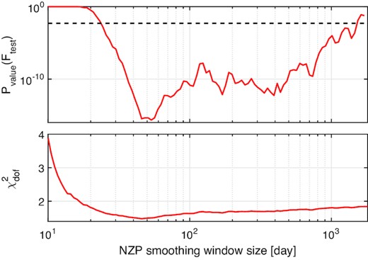
Searching for the typical time-scale of HIRES NZP variations: the upper and lower panels show the p(F_test)-value and |$\chi ^2_{\rm dof}$| statistics of subtracting a moving weighted average from the NZPs. The dashed line in the upper panel is the p-value =0.005 line, which is usually considered as the critical value for significant evidence (Benjamin et al. 2018).

We have thus adopted the 50-day moving average of the NZPs as our model for the long-term systematic RV variations in HIRES. It is plotted in Fig. 2 with a green solid line. The smoothing leads to a decrease of the effective NZP uncertainty from ∼0.74 m s⁻¹ to ∼0.29 m s⁻¹. In addition, the short smoothing window obviated the need to model the 2004 jump separately, as it can be viewed as yet another run-to-run jump, with one difference: while virtually all other jumps go stochastically up and down, the 2004 jump changed the instrument’s zero-point quasi-permanently.

Using the adopted NZP model, we corrected all HIRES RVs by subtracting the model from each RV according to its night of observation. To avoid self biasing, we calculated the NZP model for each RV-quiet star by using the RVs of all other RV-quiet stars. The model uncertainties were added in quadrature to the internal RV uncertainties. Since the adopted model averaged a few adjacent NZPs for each night, the mean model uncertainty is ∼0.3 m s⁻¹, and higher than 1.0 m s⁻¹ in nine nights only.

The mean absolute value of the correction is ∼0.6 m s⁻¹. Hence, the correction removed from the HIRES RVs a small but significant systematic effect. The correction lowered the median std (RV) of the RV-quiet stars from ∼4.7 to ∼4.6 m s⁻¹. Since their median RV uncertainty (⁠|$\overline{\delta {\rm RV}}$|⁠) is ∼1.5 m s⁻¹, we conclude that their RV scatter, even after the NZP correction, is still dominated by either intrinsic or additional systematic RV variations.

3.2 Intra-night RV drift

We used the NZP-corrected RVs and the auxiliary data of the observations to look for additional systematic effects in HIRES RVs. Using the criteria of Benjamin et al. (2018), who set the threshold for significant findings to p-value =0.005, we found one small but significant correlation: between the RVs and the time relative to local midnight (t_mid). The linear RV–t_mid correlation, shown in Fig. 4, have a p(F_test)-value of ∼3 · 10⁻⁸, and a slope of 0.051 ± 0.004 m s⁻¹ h⁻¹. For completeness, we further corrected the RVs for this small RV–t_mid correlation. We also checked whether a second or third-order polynomials would better describe the RV–t_mid relation, but found the improvement to be insignificant.

Figure 4.

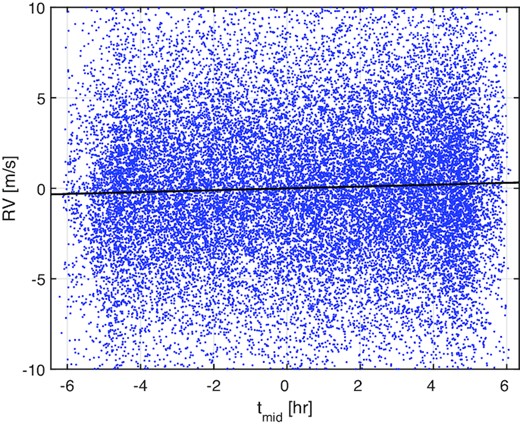
Systematic RV–t_mid correlation in HIRES: NZP-corrected RV-quiet star RVs are shown in blue, and the black line shows the adopted linear correction model, with a slope of 0.051 ± 0.004 m s⁻¹ h⁻¹. The Y-axis was limited to ±10 m s⁻¹ to enable inspecting the small-size effect.

4 THE IMPACT OF THE CORRECTION ON PERIODIC RV SIGNALS

The corrected HIRES RVs, as well as the correction values, are given in an online table.² The table has a similar format to the online version of table 1 of Butler et al. (2017), with two values appended to each line: the correction value (CV) and its uncertainty (δCV). Table 1 shows five representative lines from the online table.

Table 1.

Five representative lines from the online table of HIRES RVs corrected for small systematic errors.

Target	BJD	RV [m s−1]	δRV [m s−1]	S-index	H-index	|$\overline{n_{\rm phot}}$|	t  exp [s]	CV [m s−1]	δCV [m s−1]
GJ 3470	2456196.12775	−1820.918	2.681	1.5725	0.05486	8749	860	0.178	0.238
GJ 3470	2456203.09433	−1735.865	2.713	1.6339	0.05594	8610	914	0.545	0.267
GJ 3470	2456290.09917	451.066	3.450	1.7408	0.05560	7128	804	0.244	0.522
GJ 3470	2456325.97211	1258.111	2.792	1.7354	0.05556	8695	1139	0.339	0.258
GJ 3470	2456326.96973	1266.413	2.573	1.5718	0.05515	8711	846	0.337	0.258

Since almost all the stars with n_RV ≥ 10 had std(RV) of ≳ 2 m s⁻¹ before the correction, and since the typical correction values are ≲ 1 m s⁻¹, the correction usually had a very small effect on the RV scatter of individual stars. However, the correction does have some typical time-scales, and it is interesting to see how it impacts specific frequencies in some stellar RV power spectra.

The upper panel of Fig. 5 shows the normalized GLS periodogram (Zechmeister & Kürster 2009) of the NZPs. The three highest peaks, in descending power, belong to periods of ∼6, 500, ∼30, and ∼175 days. The lower panel of Fig. 5 shows the same periodogram, after correcting the NZPs for the 2004 jump and the long-term drift, by subtracting the 1.5 m s⁻¹ jump and a moving weighted-average filter of a 1000-day window. The correction removed all significant periodogram peaks, pushing the highest peak below a false-alarm probability (FAP) of 0.001. This indicates that the 30-day and the 175-day peaks probably emerged from the window function, coupled with the jump and the long-term NZP variations. Similarly, we expect the adopted correction, detailed in Section 3, to impact mainly long-period low-amplitude RV signals, and spurious signals arising from coupling the systematic variability with the window function of each star.

Figure 5.

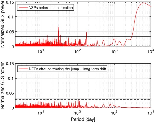
Normalized GLS periodograms of the NZPs, before and after subtracting from the NZPs the 2004 jump and the long-term drift. The dashed and solid black lines mark the 0.001 and 0.0001 FAP lines.

In order to demonstrate such effect, Fig. 6 shows the normalized GLS periodogram of the HIRES RVs of HD 10476, before and after the correction. HD 10476 appears in table 2 of Butler et al. (2017) as a planet candidate with P ∼ 5000 days and K ∼ 2 m s⁻¹. Not only the correction suppressed all periodogram peaks to higher FAP levels, it also made the 5000-day peak less significant than the shorter-period 11-day one. We believe that a repeated search for candidates, which would use the corrected RVs and a similar method to the one applied by Butler et al. (2017), might remove HD 10476 from the candidates list.

Figure 6.

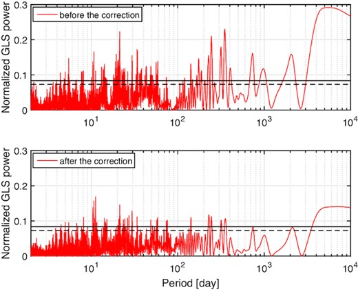
Normalized GLS periodograms of HIRES RVs of HD 10476, before and after correcting for the systematic effects. The dashed and solid black lines mark the 0.001 and 0.0001 FAP lines.

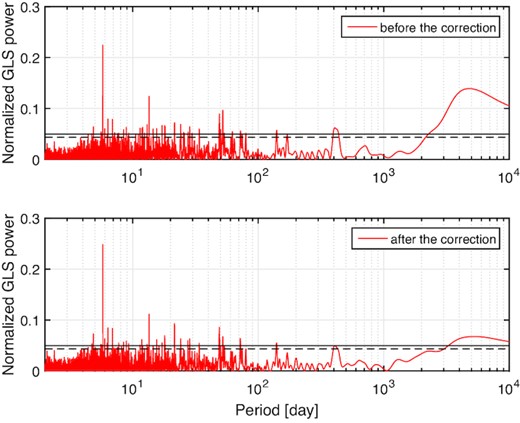
Fig. 7 shows the normalized GLS periodogram of the HIRES RVs of HD 1461, which is known to host two short-period super-Earth planets, with orbital periods of 5.77 days (Rivera et al. 2010) and 13.5 days (Díaz et al. 2016). In addition, the star is claimed to show a long-period ∼4000-day signal, probably related to activity (Díaz et al. 2016). The correction suppressed the long-period signal to an FAP level higher than the signals of the two published planets. However, it also slightly suppressed the 13.5-day signal, while the 5.77-day signal became more significant. Therefore, it could be interesting to perform combined analysis of the corrected HIRES RVs and the HARPS RVs published by Díaz et al. (2016).

Figure 7.

Same as Fig. 6, but for HD 1461.

5 SUMMARY AND CONCLUSIONS

We have presented a correction of the HIRES RVs, published by Butler et al. (2017), for two small but significant systematic effects: variations of the instrumental zero-point RV of ≲ 1 m s⁻¹, and an intra-night RV drift of ∼0.05 m s⁻¹ h⁻¹. Periodogram analysis of the NZPs, and of planet candidates from Butler et al. (2017), shows that the correction affects mainly low-amplitude (≲ 2 m s⁻¹) and long-period (≳ 2000 days) signals. We provide the exoplanet community with the corrected HIRES RVs, which are now more self-consistent over the ∼18 years of observations. To facilitate verification or reproduction of our results, the code we used to calculate the corrections is also available for download.³

The presented results suggest that repeated observations of RV-quiet stars is important even in the era of simultaneously-calibrated and stabilized RV spectrographs, and that it can reveal systematic errors well below the noise level of the instrument. The methods applied in this work are simple and straightforward. They were used successfully in the past (e.g., Campbell et al. 1988), as well as recently (e.g., Trifonov et al. 2018). They can be applied to any precision RV survey, given that enough RV-quiet stars are observed every night.

Presently, more and more precision RV instruments become operational, and the precision is being pushed to the ∼0.1 m s⁻¹ level (e.g., Fischer et al. 2016). In order to identify and correct for instrumental systematic RV errors, we urge the observatories to keep observing RV-quiet stars on a nightly basis. In addition, we encourage the different RV surveys to publish their full bank of RVs, as done by Butler et al. (2017), for the whole exoplanet community to analyse.

ACKNOWLEDGEMENTS

This research was supported by the ISRAEL SCIENCE FOUNDATION (grant no. 848/16).

Footnotes

1

Available for download at https://ebps.carnegiescience.edu/data/

2

Table of the radial velocities is available at the CDS via anonymous ftp to cdsarc.u-strasbg.fr (130.79.128.5) or via http://cdsarc.u-strasbg.fr/viz-bin/qcat?J/MNRAS/vol/page}

3

https://github.com/levtalor/correcting-hires-Keck-data

APPENDIX: NZP CALCULATION METHOD

To avoid overweighting a single star in a given night, we first binned repeated observations of the same star in a given night by taking the weighted average of its RVs in that night, and its RV scatter in that night as its RV error. Then, we subtracted, from each-star RVs, its-own weighted-average RV, μ_k, with the weights calculated from its internal RV uncertainties as |$\delta {\rm RV}_k^{-2}$|⁠. The average-RV uncertainty was calculated via

\begin{eqnarray*} \delta \mu _k = {\rm max}\lbrace \left (\sum _k{\rm \delta {\rm RV}_{k}^{-2}}\right)^{-0.5},{\rm wstd}_k \cdot n_{{\rm RV}}^{-0.5}\rbrace , \end{eqnarray*}

(A1)

where wstd_k is the weighted std of its RVs. Then, δμ_k, was added in quadrature to its RV uncertainties. This way we down-weighted the RVs of low-quality RV-quiet stars. The NZP of each survey night (NZP_n) was taken as the weighted-average RV of the RV-quiet stars observed that night, after removing 10σ_k outliers per star and 5σ_n outliers per night, as long as they deviated by >10 m s⁻¹ from the mean. To avoid underestimating δNZP_n, regardless whether the RV scatter of that night was dominated by intrinsic scatter or by the δRVs of the observed stars, we took

\begin{eqnarray*} \delta {\rm NZP}_n = {\rm max}\lbrace \left (\sum _k{\rm \delta {\rm RV}_{k,n}^{-2}}\right)^{-0.5},{\rm wstd}_n \cdot n_{{\rm RV},n}^{-0.5}\rbrace , \end{eqnarray*}

(A2)

where n_{RV, n} is the number of RVs used to calculate the NZP of night n, and wstd_n is the weighted std of the RVs in that night.

We note that the boundary between RV-quiet and RV-loud stars can be shifted to a value lower than 10 m s⁻¹, at the cost of reducing the number of stars used for the calculations. In addition, RV-quiet stars with true orbital or activity-induced signals were not excluded from NZP calculations. Replacing their RVs with their RV residuals, after subtracting a model for the true variation, is a possible improvement we consider for our algorithm.

Another possible improvement of the algorithm is to model μ_k and the NZPs simultaneously by maximizing the likelihood

\begin{eqnarray*} \ln L = \sum _{k,n}\frac{{\rm RV}_{k,n}-\mu _k-{\rm NZP}_n}{\delta {\rm RV}_{k,n}^2+\sigma _k^2}, \end{eqnarray*}

(A3)

where |$\sigma _k^2$| is the so-called RV jitter, which should take into account unknown low-amplitude variations due to stellar activity or orbit. Such an approach has the advantage of a self-consistent weighting of each-star RVs. However, it is computationally heavy, and estimating δNZP_n is not straightforward.