Uncovering the key dimensions of high-throughput biomolecular data using deep learning

Abstract

Recent advances in high-throughput single-cell RNA-seq have enabled us to measure thousands of gene expression levels at single-cell resolution. However, the transcriptomic profiles are high-dimensional and sparse in nature. To address it, a deep learning framework based on auto-encoder, termed DeepAE, is proposed to elucidate high-dimensional transcriptomic profiling data in an encode–decode manner. Comparative experiments were conducted on nine transcriptomic profiling datasets to compare DeepAE with four benchmark methods. The results demonstrate that the proposed DeepAE outperforms the benchmark methods with robust performance on uncovering the key dimensions of single-cell RNA-seq data. In addition, we also investigate the performance of DeepAE in other contexts and platforms such as mass cytometry and metabolic profiling in a comprehensive manner. Gene ontology enrichment and pathology analysis are conducted to reveal the mechanisms behind the robust performance of DeepAE by uncovering its key dimensions.

INTRODUCTION

High-throughput transcriptomic profiling, also known as gene expression profiling, has been widely adopted as the tool to characterize gene expression patterns in different cellular states under various disease conditions (1), drug treatments (2,3), and genetic perturbations (4). The genome-wide single-cell transcriptomic profiling can measure tens of thousands of genes in a high-throughput cell-by-cell basis manner (5) and provide rich genetic information for subsequent studies. In pathological diagnosis, Nelson et al. (6) tested whether the miRNA expression variations detected in human brain tissue were associated strongly to dementia with Lewy body pathology through gene expression profiling techniques. Similarly, Olah et al. (7) confirm the existence of an aging-related microglial phenotype in the aged human brain and its involvement in the related pathological processes based on microglia transcriptomic profiling. For translational research, Huet et al. (8) harness gene-expression profiling data to build and validate a predictive model for diagnosing the patients with follicular lymphoma. Based on gene expression profiles, Prabhakaran et al. (9) developed a unique 12-chemokine gene expression score to stratify breast cancer patients based on intratumoral immune composition. In addition, gene expression profiles have been widely adopted in drug discovery and drug-target network construction; for instance, Bagot et al. (10) analyzed the gene expression data in four interconnected limbic brain regions implicated in depression and its treatment with imipramine or ketamine; Zickenrott et al. (11) proposed a differential network approach for identifying candidate target genes and chemical compounds for disease research based on transcriptomics.

Various transcriptomic technologies have been developed to measure messenger RNA (mRNA) levels based on DNA microarrays and sequencing technologies. By now, the high-throughput sequencing platforms have already replaced microarrays as the tool of choice for high-throughput gene expression profiling. Specifically, single-cell RNA-seq enables researchers to identify active genes in each cell (12). Although those breakthroughs in transcriptomics have made it possible to profile single-cell transcriptomics, the single-cell RNA-seq data have brought new challenges in data acquisition, storage, computation, and analysis. A crucial challenge in gene expression profiling is its high dimensionality since there are more than 20 000 genes in each human genome for high-throughput profiling. In addition, many emerging applications require massive numbers of profiles up to hundreds of thousands or more for statistical significance. For instance, Ho et al. (13) obtained ∼90 000 reads from more than 5000 expressed genes in ∼6500 cells using single-cell RNA-seq to identify the markers of resistance to targeted BRAF inhibitors in melanoma cell populations; a gene expression matrix of 13 160 genes across 4233 filtered zebrafish cells was derived for comprehensive identification and spatial mapping of habenular neuronal types (14); Herring et al. (15) sequenced 2402 colonic cells with an average of 49 680 reads per cell to reveal alternative tuft cell origins in the gut.

To address the above issues, dimensionality reduction techniques have been leveraged during the gene expression data collection, interpretation, and analysis for two-fold objectives: computational and statistical tractability can be ensured and noises can be reduced while preserving the intrinsically low-dimensional signals of interest (16,17). In some cases, principal component analysis (PCA) is often used to project gene expression data by a linear combination of the original gene expression values with the largest variances. However, PCA has a shortcoming that, for real datasets, the first and second principal components tend to depend on the proportion of genes detected per cell (16,18). Moreover, the single-cell RNA-seq data have noises caused by the transcriptional burst effects or low amounts (i.e. the dropout events) of RNA transcripts. Hence, those sparsity and nonlinearity make the PCA inefficient for single-cell RNA-seq data. In addition to PCA, independent components analysis (19), Laplacian eigenmaps (20), and t-distributed stochastic neighbor embedding (t-SNE) (21–23) are also popular dimensionality reduction technicques in high-dimensional gene expression data. Uniform manifold approximation and projection (UMAP) is a new algorithm recently published by McInnes et al. (24). It has been experimentally verified that UMAP shows equally meaningful representations compared with t-SNE. After that, Becht et al. have raised an issue on incremental data learning to an existing embedding (25). Recently, Scvis was proposed as a robust latent variable model in a probabilistically generative manner (26). In addition, several studies have been proposed to impute the expression levels of unmeasured (unobserved) genes from a small number of landmark genes (∼1000) by leveraging computational methods (27–29). Those methods assume that, within a large number of genes (∼22 000) across the whole human genome, most profiles share similar expression patterns (17).

Therefore, Cleary et al. (17) proposed a computational method (published on Cell) based on compressed sensing (30,31), in which the expression data can be collected in a compressed format. It is composed of two phases: compression and decompression. In compression, it projects the high-dimensional expression data into low-dimensional space as a composite measurement of linear combinations of genes. The gene expression data can be collected in a compressed format. In decompression, the high-dimensional expression profiles (∼20 000) can be recovered from a few (up to 100-fold fewer than the number of genes or reads) composite measurements by leveraging two properties: (i) gene set modularity; (ii) gene expression sparsity (17). The recovered expression profiles produced by CS-SMAF (Compressed Sensing-Sparse Module Activity Factorization) were demonstrated consistent with the wet-lab profiles. The CS-SMAF not only provides efficient storage (composite measurements) for the collected high-dimensional data but also can be leveraged to recover gene expression profiles. The CS-SMAF involves an iterative process of LASSO (32) and orthogonal matching pursuit (OMP) (33) to identify the sparse module dictionary and active module activity. Obviously, the iterative LASSO and OMP cannot optimize such a non-convex problem that limits the recovery accuracy. Hence, we seek to develop a computational approach with accurate and robust performance.

Recently, deep learning has been successfully implemented in various machine learning tasks and has been demonstrated for its capability in learning hierarchical and nonlinear patterns (34). In addition, deep learning models (i.e. deep neural networks, convolutional neural networks, recurrent neural networks, and auto-encoder) are scalable and highly flexible to large-scale data problems. With those advances, it has achieved ground-breaking performance in various well-studied topics, such as natural language processing, computer vision (35), board game programs (AlphaGo) (36) , and machine translation. Moreover, deep learning has been an exciting and promising method in molecular genetics (37), such as promoter and enhancer recognition (38), RNA splicing prediction (39) , and transcription factors binding sites prediction (40). Eraslan et al. (41) proposed a deep count autoencoder network to denoise single cell RNA-seq datasets with an advantage of data imputation in quality and speed. AutoImpute (42) applied autoencoder to impute the sparse gene expression matrix caused by dropout events. VASC (43) based on autoencoder provides dimension reduction and visualization on single cell RNA-seq data with superior performance. Those deep learning models show remarkable performance and scalable flexibility as a powerful alternative for encoding high-dimensional gene expression profiles. Although the autoencoder performs well in data compression (dimension reduction) and reconstruction, its model interpretability is a major weakness since the autoencoder itself is known as a black-box method.

In this study, we propose a deep neural network framework, termed DeepAE, to identify the key dimensions of high-dimensional gene expression profiles. DeepAE is composed of encoder and decoder phases for compression and decompression respectively. The encoder phase aims at compressing (or encoding) the gene expression data in a non-linear format such that, in contrast to the linear compression of CS-SMAF, it can preserve the nonlinear patterns of the high-dimensional gene expression. The decoder phase aims at decompressing (or decoding) the transcriptomic profiling data. In addition, we also investigate the performance of DeepAE in other biotechnologies, such as mass cytometry and metabolic profiling. After that, we propose a method to identify and explain the key dimensions from the central hidden layer of DeepAE in terms of its functions and pathology.

MATERIALS AND METHODS

In this section, we introduce the transcriptomic datasets of interest. After that, we propose the DeepAE model for the compression and decompression of high-dimensional gene expression data. For comparisons, we discuss the related methods and the performance evaluation metrics.

Datasets

We have adopted nine single-cell RNA-seq datasets from Gene Expression Omnibus (GEO) as the benchmark datasets in this study. Table 1 summaries the nine gene expression datasets from single-cell RNA-seq including the GEO accession number, organism, the number of genes (or probes), the number of cell samples, and the publication venues. The nine gene expression datasets are collected from three species: HomoSapiens (GSE71858, GSE52529, GSE77564, and GSE69405), MusMusculus (GSE60361, GSE62270, GSE48968, and GSE78779), and SaccharomycesCerevisiae (GSE102475). For the dimension of genes (or probes), most of the gene expression datasets have more than 10 000 dimensions except GSE102475. For the sample dimension (i.e. cell dimension), most are ranged from 100 to 600. In particular, GSE77564 has the fewest cell samples (=20) while GSE60361 has the largest cell samples (>3000).

Table 1.

Summary of the nine benchmark gene expression datasets

GEO Accession	Species	Genes (Probes)	Cell Samples	Journal
GSE60361 (23)	M. Musculus	19 972	3005	Science
GSE65525 (58)	M. Musculus	24 175	2717	Cell
GSE62270 (59)	M. Musculus	23 630	288	Nature
GSE48968 (60)	M. Musculus	10 972	564	Nature
GSE52529 (61)	H. Sapiens	47 192	372	Nature Biotechnology
GSE84133 (62)	M. Musculus	14 878	1886	Cell Systems
GSE78779 (63)	M. Musculus	22 814	96	Genome Biology
GSE69405 (64)	H. Sapiens	57 820	201	Genome Biology
GSE102475 (65)	Saccharomyces	6789	163	PLoS Biology

Auto-encoder

Auto-encoder is an artificial neural network to identify the efficient representation (i.e. key dimensions) of high-dimensional data. The structural form of the auto-encoder is a feed-forward neural network composed of encoding and decoding. We can mathematically define these two phases as mappings displayed in equation (1). The mapping is conducted by projecting the input data vector with the weight matrix W, bias term b, and the non-linear activation operation (σ) such as sigmoid and tanh. In a basic auto-encoder, it contains an input layer, an output layer, and a hidden layer in between. The output layer has the same number of neurons as the input layer to identify the key dimensions from the hidden layer. The hidden layer is smaller than the input layer; it enables the model to create the compressed representation of input data in the hidden layer through the encoding (ϕ: X → Z). In addition, the auto-encoder can recover the input layer X by generating a reconstructed input X′ (output layer) through minimizing the difference between input X and output X′ called decoding (φ: Z → X′). Since the auto-encoder can force the networks to compress the high-dimension data into a low-dimension representation which captures the non-linear relationships within the original data, it can thus be adopted for massive dimensionality reduction and data compression. For instance, large image reconstruction (44), health state identification (signal data) (45), and transcriptomic machinery representation (46). Exploiting such advantages, we would like to explore the auto-encoder potential on the interpretation of high-dimensional transcriptomic profiles.

$$\begin{equation*} \begin{aligned} \phi &: X \rightarrow Z: x\longrightarrow \phi (x)=\sigma (Wx+b)=z\\ \varphi &: Z \rightarrow X^{\prime }: z\longrightarrow \varphi (z)=\sigma (\widetilde{W}z+\widetilde{b})=x^{\prime } \end{aligned} \end{equation*}$$

(1)

DeepAE

In this section, we describe the main elements of the proposed DeepAE. We describe how such deep learning networks interpret the high-dimensional gene expression data. The DeepAE is trained by n cell samples X = {x¹, x², ..., xⁱ, ..., xⁿ} where each sample xⁱ consists of g genes (i.e. attributes or probes) |$x^i = \lbrace x_{1}^{i}, x_{2}^{i}, ..., x_{j}^{i}, ..., x_{g}^{i}\rbrace$|⁠. Thereby, |$x_{j}^{i}$| denotes the j-th gene (probe) of the i-th sample. Figure 1 illustrates a schematic view of the proposed DeepAE neural network. It consists of one flattened input layer representing the original gene expression profiles, multiple hidden layers, and one output layer representing the reconstructed gene expression profiles. The encoder (dotted blue box) is composed of the input layer and multiple hidden layers, while the decoder (dotted red box) consists of the output layer and the remaining hidden layers. The central hidden layer refers to the compressed data in both encoder and decoder. All hidden layers have different numbers of hidden units. The neural connections between layers are fully connected.

Figure 1.

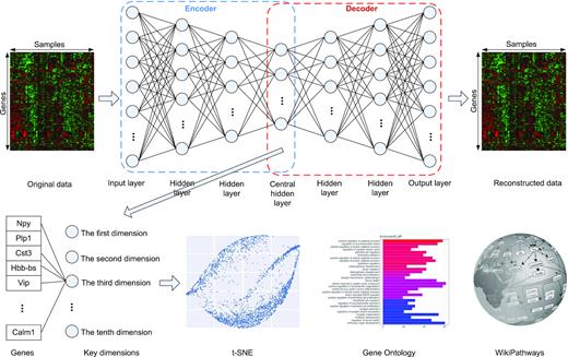
Overview of the proposed DeepAE. It consists of one input layer representing the original gene expression profiles, multiple hidden layers, and one output layer representing the reconstructed gene expression profiles. The encoder (dotted blue box) is composed of input layer and half hidden layers, while the decoder (dotted red box) consists of the output layer and the rest of hidden layers. The central hidden layer refers to the compressed data in both encoder and decoder. All the hidden layers have different hidden units. The neural unit connections between layers are fully connected.

The DeepAE is a multi-layer feedforward neural network composed of two non-linear mappings (i.e. encoding and decoding). The encoder and decoder form a symmetrical architecture with nine layers of neurons; each layer is followed by a nonlinear function and its parameters θ. The encoder mapping ϕ_θ( · ) maps an input vector sample xⁱ to a compressed representation |$z$|ⁱ in the latent space Z. The latent representation |$z$|ⁱ is then mapped back by the decoder φ_θ( · ) to a reconstructed vector |$\hat{x}_i$| of the original input high-dimensional space. The non-linear encoder and decoder mapping of the DeepAE encompassing several neuron layers can be formally defined as below.

$$\begin{eqnarray*}\phi _{\theta }^{l}(\cdot ) & = &\sigma ^{l}(W^{l}(\phi _{\theta }^{l-1}(\cdot ))+b^{l})\;,\\ \varphi _{\theta }^{l}(\cdot ) & = &\sigma ^{l}(\widetilde{W}^{l}(\phi _{\theta }^{l-1}(\cdot ))+\widetilde{b}^{l})\;\;. \end{eqnarray*}$$

(2)

where σ denotes the non-linear activation function such as sigmoid or tanh functions, θ denotes the model parameters, |$\lbrace W, b, \widetilde{W}, \widetilde{b}\rbrace$|⁠, |$\lbrace W\in \mathbb {R}^{d_z \times d_x}, \widetilde{W}\in \mathbb {R}^{d_x \times d_z}\rbrace$| denote the weight matrices, |$\lbrace b\in \mathbb {R}^{d_z}, \widetilde{b}\in \mathbb {R}^{d_x}\rbrace$| denote the offset bias vectors, and l denotes the layer index.

In this study, the leaky ReLU function is adopted as the non-linear activation function in all hidden layers and the output layer as shown below.

$$\begin{equation*} \sigma (x) = {\rm leaky}\_ReLU(x) =\left\lbrace \begin{array}{@{}l@{\quad }l@{}}x & \text{ if } x>0 \\ \alpha x & \text{ if } x\le 0 \end{array}\right.\;. \end{equation*}$$

(3)

where α represents the non-zero gradient which is usually set to 0.01.

The DeepAE is trained to learn the optimal model parameters θ that minimize the difference between the original gene expression data xⁱ and its reconstruction |$\widetilde{x}^i = \varphi _{\theta }(\phi _{\theta }(x^i))$|⁠. Thus, the average sum is formulated as the loss function as shown below.

$$\begin{equation*} {\rm Loss}(x^i, \widetilde{x}^i) = \frac{1}{g}\sum _{j=1}^{g}|x^{i}_{j}-\widetilde{x}^{i}_{j}|\;. \end{equation*}$$

(4)

CS-SMAF and other benchmark methods

The early work, CS-SMAF published on Cell, leveraged the compressed sensing from signal processing to project the high-dimensional gene expression profiles into low-dimensional gene modules; Cleary et al. (17) proposed to identify the sparse module dictionary and sparse module activities from the high-dimensional data using matrix factorization. Thus the SMAF refers to finding the gene-modular activities from the high-dimensional gene expression data.

In addition, we also consider other existing matrix factorization methods as the benchmark methods including the Singular Value Decomposition (SVD) (47), k sparsity Singular Value Decomposition (k-SVD) (48), and sparse Non-negative Matrix Factorization (sNMF) (49). Those benchmark methods are all commonly used matrix factorization methods. SVD is unconstrained, while k-SVD is constrained to manually set k eigenvectors. However, SVD and k-SVD suffer from the limitation that they are not suitable to sparse data. The sparsity-enforcing methods sNMF and CS-SMAF can generate sparse solutions (17). Most importantly, CS-SMAF can generate compact, sparse, and distinctive dictionaries, whereas the dictionaries generated from SVD and sNMF are largely redundant (17). As aforementioned, the CS-SMAF involves an iterative process of LASSO and OMP that cannot optimize such a non-convex problem, limiting the recovery accuracy. We introduce them into the context of compressed sensing to identify the non-negative, sparse module dictionary, and sparse module activities from the high-dimensional gene expression data.

Performance evaluation metrics

In this study, three evaluation metrics are computed to measure the encoding performance between the original high-dimensional gene expression data and the reconstructed gene expression data: Pearson Correlation Coefficient (PCC), Euclidean Metric (EM), and Mean Absolute Error (MAE) as shown below.

$$\begin{equation*} PCC_{X,X^{\prime }}=\frac{Cov(X,X^{\prime })}{\sigma _X \sigma _{X^{\prime }}}\;. \end{equation*}$$

(5)

$$\begin{equation*} EM = \sqrt{\sum _{i=1}^{n}\sum _{j=1}^{g}(X_{ij}-X^{\prime }_{ij})^2}\;. \end{equation*}$$

(6)

$$\begin{equation*} MAE = \frac{1}{gn}\sum _{i=1}^{n}\sum _{j=1}^{g}|X_{ij}-X^{\prime }_{ij}|\;. \end{equation*}$$

(7)

where n and g represent the numbers of rows and columns in X^{n × g} and X^{′n × g}.

PCC is ranged from −1 to 1, indicating the linear correlation between X and X′. The value of 1 (or −1) indicates total positive (or negative) linear correlation, while 0 indicates the absence of linear correlation. EM and MAE are two commonly used methods to evaluate the two matrices’ distance and errors.

RESULTS

In this section, we built the proposed models on nine gene expression datasets collected from GEO (https://www.ncbi.nlm.nih.gov/geo/). We show the implementation details of DeepAE and its compression and decompression performance on high dimensional gene expression profiles. In addition, we explore the applications of DeepAE in other high-throughput biomolecular contexts such as metabolic profiling and mass cytometry. Source code implemented in Python can be found at https://github.com/sourcescodes/DeepAE.

Implementation details and model selection

We experimented four distinct neural network architectures to identify the best DeepAE model. Table 2 tabulates the overview of those architectures. The Leaky ReLU function is adopted as the non-linear activation function in all hidden layers and the last (output) layer where α is set to 0.2. The Adam algorithm is adopted as the optimization method for back-propagation to minimize the cost function (equation 4) with the hyper-parameters β₁ = 0.9, β₂ = 0.999, and ε = 1e − 08. The initial learning rate is set to 0.0001. The number of iterations to train the model is set to 1000. We apply the DeepAE model to each dataset where 5% of samples for training and 95% for testing. Each dataset is randomly divided into the training set and testing set with distinct random seeds. Each experiment was run five times for robust performance estimation.

Table 2.

The proposed architectures ranging from the shallow architecture with a single fully connected hidden layer to the deep architecture with seven hidden layers

Architectures	Number of Neurons in Each Layer
DeepAE1	[Input layer]-50-[Output layer]
DeepAE2	[Input layer]-256-50-256-[Output layer]
DeepAE3	[Input layer]-640-256-50-256-640-[Output layer]
DeepAE4	[Input layer]-1280-640-256-50-256-640-1280-[Output layer]

To identy the best DeepAE model, we tested the four architectures as shown in Table 2 on the nine single-cell RNA-seq datasets summarized in Table 1. Supplementary Table S1 tabulates the performance comparison of the four distinct DeepAE architectures evaluated in three metrics: PCC, EM, and MAE. The best performance on each dataset is highlighted in bold. In Supplementary Table S1, the DeepAE4 with seven hidden layers outperforms other DeepAE architectures on all single-cell RNA-seq datasets except GSE69405. For the evaluation metric PCC, all DeepAE models exceed 80%. In addition, DeepAE4 achieves 97.03% (±0.7%) on GSE77564. We also tried two extra-deep architectures (DeepAE5 [Input layer]-2580-1280-640-256-50-256-640-1280-2580-[Output layer] and DeepAE6 [Input layer]-2580-1280-640-256-128-50-128-256-640-1280-2580-[Output layer]). We test those two extra-deep architectures on GSE84133 and GSE65525. In addition to calculating PCC, EM and MAE, we also evaluate the running time to compare with DeepAE4. The results from Supplementary Table S2 shows that, for GSE84133, DeepAE5 slightly outperforms DeepAE4 and DeepAE6 in PCC, EM and MAE, while its running time is increased significantly from 1445.55 sec (DeepAE4) to 2542.33 sec (DeepAE5); for GSE65525, DeepAE4 outperforms other two architectures in all four metrics. The observed results show that the auto-encoder depth is the key factor to recover the high-dimensional sparse structure within each profiling dataset. Therefore, we select DeepAE4 (architecture: [Input layer]-1280-640-256-50-256-640-1280-[Output layer]) as the final model, consistent with the consensus gene regulation hierarchy as observed from the ENCODE project (50).

Performance on transcriptomic profiling data

In this section, we applied the proposed DeepAE model to compress and decompress the high-dimensional transcriptomic profiles. The DeepAE consists of seven hidden layers and the architecture is [Input layer]-1280-640-128-50-128-640-1280-[Output layer]. The central hidden layer (also called latent space) has 50 units corresponding to the key dimensions. We use ‘measurements’ to represent the learned key dimensions. Taking the advantages of compressed sensing, CS-SMAF can compress the gene expression data from high-dimensional levels (∼20 000) into low-dimensional space (∼100) and then can reconstruct it with good quality. In the model selection section, we have investigated the possibility to compress the gene expression data to 50 dimensions with the proposed DeepAE models. Hence, in this section, we conduct the performance comparison of the proposed DeepAE and the benchmark methods. Moreover, we would like to explore the possibility to compress the gene expression levels into lower key dimensions (measurements = 25 or even 10). To rigorously estimate its performance, several methods are also considered as the benchmark methods, including SVD (47), k-SVD (48), and sNMF (49).

Supplementary Table S3 tabulates the performance comparisons of the proposed DeepAE and benchmark methods for reconstructing the high-dimensional transcriptomic profiling data from the learned lower space representations. We randomly select 5% samples as the training set and 95% samples as the testing set. Each method was run five times on each dataset as shown in Supplementary Table S3. The best performance on each dataset is highlighted in bold. The results from Supplementary Table S3 reveal that, at the same compression level (measurement = 50), the proposed DeepAE outperforms the benchmark methods across all nine transcriptomic profiling datasets. Supplementary Table S4 tabulates the pair-wise statistical significance results after comparing DeepAE with each benchmark method on nine transcriptomic profiling datasets in all metrics by t-test. All P-values in EM and MAE on each dataset are significant (p<0.01). In PCC, most P-values are <0.05 except few cases. Table 3 tabulates the average performance comparisons across nine transcriptomic datasets. On average, the DeepAE can achieve 90.56% in Pearson correlation (PCC) while the best benchmark method (sNMF) can only achieve 85.53%. Moreover, the DeepAE has significant advantages in reducing the recovery errors (EM and MAE). The DeepAE reduces the recovery errors by 50% in EM and 75% in MAE.

Table 3.

Average performance comparisons of DeepAE and benchmark methods on nine single-cell RNA-seq datasets (measurements = 50)

Metrics	SVD	k-SVD	sNMF	CS-SMAF	DeepAE
PCC	0.7708	0.8428	0.8553	0.8561	0.9056
EM	1.939E + 06	1.939E + 06	1.933E + 06	1.931E + 06	9.836E + 05
MAE	1.353E + 06	1.352E + 06	1.347E + 06	1.345E + 06	3.693E + 05

The best performance is highlighted in bold.

In addition, we investigated the possibility of DeepAE to compress the high-dimensional gene expression data from high-dimensional levels (∼20 000) into lower levels (measurements = 25 or even 10) and then recover the full data for robust performance estimation. Figures 2, 3, and Supplementary Figure S1 depict the performance comparisons among the proposed DeepAE and benchmark methods on nine single-cell RNA-seq datasets with distinct measurements (10, 25, 50, and 100) in PCC, EM, and MAE separately. From Figure 2, we can observe that the PCC values of DeepAE are always solid and robust as the measurements are decreased from 100 to 10 key dimensions. The benchmark methods, however, exhibit significant performance degradation as the measurements are decreased with significant performance deviation and sensitivity on each dataset. From Figure 3 and Supplementary Figure S1, none of the recovery error metrics (EM and MAE) shows significant fluctuations; the EM and MAE of DeepAE are still significantly lower than benchmark methods across all datasets. Figure 4 presents the average performance comparisons of DeepAE and benchmark methods on all datasets with measurements decreasing from 100 to 10. The DeepAE can keep the Pearson correlation (PCC) over 90% without any noticeable fluctuation. All benchmark methods have been degraded to varying degrees. Only CS-SMAF can retain the PCC above 80% among the benchmark methods. Therefore, the proposed DeepAE shows robust performance in reconstructing the high-dimensional expression profile from the compressed space by identifying the key dimensions.

Figure 2.

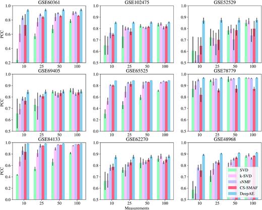
Performance comparisons of the proposed DeepAE and benchmark methods on nine single-cell RNA-seq datasets with distinct measurements (10, 25, 50, and 100) evaluated in PCC metric. Each bar height stands for the mean performance value across multiple runs, and the black line on the top of bar denotes the standard deviation; the Y-axis scale of sub-figure (GSE60361, GSE66525, and GSE84133) is different from other sub-figures to accommodate the performance of SVD. The benchmark methods include SVD (47), k-SVD (48), sNMF (49), and CS-SMAF (17).

Figure 3.

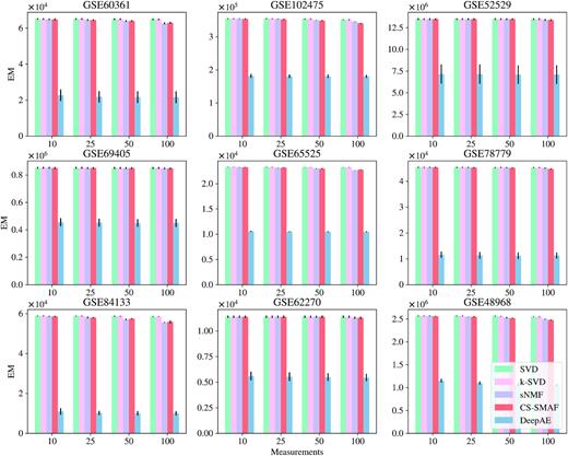
Performance comparisons of the proposed DeepAE and benchmark methods on nine single-cell RNA-seq datasets with distinct measurement (10, 25, 50, and 100) evaluated in EM metric. Each bar height stands for the mean performance value across multiple runs, and the black line on the top of bar denotes the standard deviation; the Y-axis scale of sub-figure is different from each other. The benchmark methods include SVD (47), k-SVD (48), sNMF (49), and CS-SMAF (17).

Figure 4.

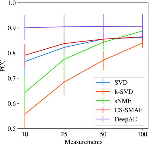
Average performance comparisons of the proposed DeepAE and benchmark methods on nine single-cell RNA-seq datasets with distinct measurements (10, 25, 50, and 100) evaluated in PCC metric.

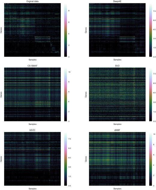
To illustrate the performance of the proposed DeepAE and benchmark methods on transcriptomic profiling data, we depict an example of these methods on reconstructing high-dimensional gene expression profiles from its learned lower space. Figure 5 consists of the original high-dimensional gene expression profiles (GSE60361) and the profiles reconstructed from the proposed DeepAE and benchmark methods including SVD (47), k-SVD (48), sNMF (49), and CS-SMAF (17) with measurements = 10. The high-dimensional gene expression profiles are processed with log(data + 1). Heatmaps in Figure 5 show the gene expression patterns and the hierarchical clustered samples and genes. Each row corresponds to a specific gene; each column corresponds to a particular cell sample. White to green colours suggest high to middle expression whereas green to black colours suggest low to null expression. In Figure 5, each method has varying degrees of information loss while DeepAE can preserve most of the original gene expression patterns.

Figure 5.

Original gene expression profiles (GSE60361) and the profiles reconstructed by DeepAE, SVD (47), k-SVD (48), sNMF (49), and CS-SMAF (17). The data in the heatmaps is processed with log(data + 1).

We also run the proposed DeepAE and benchmark methods on single cell RNA-seq datasets with smaller measurements (5, 2, and 1). The datasets are all preprocessed with z-score normalization. Supplementary Figure S5 illustrates the results on GSE84133, GSE65525, and GSE60361. We can find that, for the PCC metric, DeepAE shows a slight performance degradation when the measurement is dropped from 100 to 1, while the benchmark methods are decreased significantly; for EM and MAE, the DeepAE demonstrates slight error elevations when the measurement is dropped from 100 to 1. The gene expression profiles reconstructed from benchmark methods contain many zeros or very close to zeros while the linear correlations (measured by PCC) are sensitive to the highly expressed cells.

We have run the proposed DeepAE and benchmark methods on single-cell RNA-seq datasets with 1 to 100 measurements based on a new performance metric (Spearman correlation coefficient), instead of the PCC one. Spearman correlation coefficient can measure the non-linear relationship between two vectors which can be orderly flattened from two matrices respectively. The datasets are all preprocessed with z-score normalization. Supplementary Figure S6 illustrates the results on GSE84133 and GSE60361. We can observe that, for the Spearman metric, DeepAE does show a significant performance degradation when the measurement is dropped from 100 to 1 if we measure the performance in Spearman correlation coefficient instead of the PCC one. It implies that DeepAE mainly works by capturing the absolute magnitudes (z-scores here) of the input biomolecular data, explaining the good performance as measured in the PCC one. Model overfitting is not an issue here since the current objective is to reduce dimensions with independent test set instead of classification or clustering.

To examine it further, we have visualized the central hidden layers (encoded data) of DeepAE with the measurement = 1, 2, 5, and 10 on GSE60361 in Supplementary Figure S7. The heatmaps reflect that DeepAE can retain gene expression patterns to varying degrees with different measurements = 1, 2, 5, and 10 in absolute magnitudes. The proposed DeepAE model contains four encode hidden layers, one central hidden layer, and four decode hidden layers. After training process, each hidden layer has preserved all parameters (weights and biases) that contribute to encode (from high dimensions to its low space) and decode (from low dimensions to its original space) the testing data.

Performance on metabolic profiling data

Metabolomics describes the profiling of small molecular metabolites in a biological sample, including body fluids (urine, blood, saliva), tissues, and exhalation (51). Recent technological advances have made it possible to perform high-throughput profiling on large amounts of metabolites in biological samples. In this section, we investigate the potential of DeepAE to encode and decode the metabolic profiling data in a compressed format by identifying the key data dimensions. Two metabolic profiling datasets were collected from the hepatic steatosis of obese mice (25 806 genes and 29 samples) (52) and the irradiated leaves response to UV-B in maize (43 451 genes and 136 samples) (53). Figure 6 illustrates the performance comparisons between DeepAE and benchmark methods on those metabolic profiling datasets. The proposed DeepAE outperforms the benchmark methods in all metrics of interest. In addition, DeepAE shows robust key dimension identification performance with the decreasing compressed levels (measurements decreasing from 100 to 10).

Figure 6.

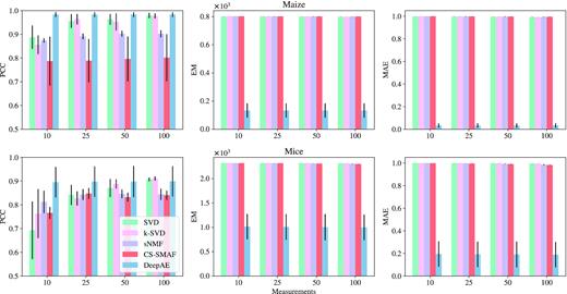
Performance comparisons among the proposed DeepAE and benchmark methods on two metabolic profiling datasets with different numbers of measurements (10, 25, 50, and 100). Each bar height denotes the mean performance value across multiple runs and the black line on the top of bar denotes the standard deviation; the Y-axis scale of each sub-figure is different from each other. The benchmark methods include SVD (47), k-SVD (48), sNMF (49), and CS-SMAF (17). Note that PCC is positively correlated to the performance while EM and MAE are negatively correlated to the performance.

Performance on mass cytometry data

Mass cytometry is a relatively new and promising technology for high-dimensional multi-parameter single cell analysis (54). Mass cytometry can provide unprecedented multidimensional single cell profiling and has recently been applied to medical fields including immunology, hematology, and oncology (55). However, the high dimensionality, large data size, and non-linearity of mass cytometry data also bring great challenges in data collection and analysis (54). In this section, we apply the proposed DeepAE to encode the mass cytometry data in a compressed manner and recover it with quality. The mass cytometry dataset analyzed in this study is derived from a project (56) and is publicly available on Cytobank (https://community.cytobank.org/cytobank/experiments/68981). We chose the mass cytometry data of MDA-MB-231 cells measured at the control time point (0 min). This mass cytometry data consists of 3452 rows (i.e. cells) and 57 columns (i.e. features). Figure 7 illustrates the performance comparisons of DeepAE and benchmark methods on mass cytometry data. The proposed DeepAE outperforms the benchmark methods in all metrics, similar to the previous datasets.

Figure 7.

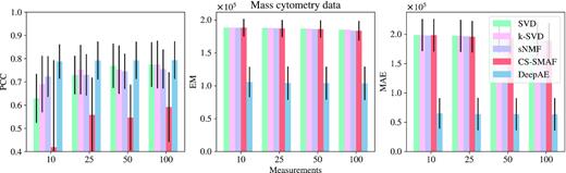
Performance comparisons among the proposed DeepAE and benchmark methods on mass cytometry dataset with different numbers of measurement (10, 25, 50, and 100). Each bar height stands for the mean performance value across multiple runs, and the black line on the top of bar denotes the standard deviation; the Y-axis scale of sub-figure is different with each other. The benchmark methods include SVD (47), k-SVD (48), sNMF (49), and CS-SMAF (17). Note that PCC is positively correlated to the performance while EM and MAE are negatively correlated to the performance.

Biological analysis on the central hidden layer of DeepAE

The aforementioned subsections showed the key dimension identification performance of the proposed DeepAE and benchmark methods on transcriptomic profiling data, mass cytometry data, and metabolic profiling data. We also investigated the robustness of DeepAE when the compression level (measurements) is dropped from 100 to 10. In this section, we would like to infer biological insights from the key dimensions of the DeepAE models.

First, we use the fully trained DeepAE to compress the original high-dimensional expression data (∼20 000) into 10 key dimensions (measurements = 10). After that, we visualize the original data and the compressed data across all samples (columns) using t-SNE (57). We expect that the compressed data can be close to the original data. Figure 8 and Supplementary Figure S2 illustrate the visualization results on the original data (∼20 000 dimensions) and compressed data (10 dimensions) of nine transcriptomic profiling datasets listed in Table 1. We can observe that the compressed data can still preserve the main topological patterns of the original data.

Figure 8.

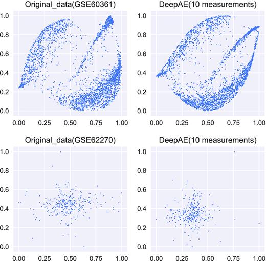
2D Visualization on the Key Dimensions (Measurements) using t-SNE between the original data (∼20 000 dimensions) and compressed data (10 dimensions) from the transcriptomic profiling datasets (GSE60361 and GSE62270).

In addition, we explained each hidden key dimension in the central hidden layer (10 dimensions) one by one biologically. In our DeepAE model, each node in the input layer represents a gene and the high-dimensional input layer is compressed into the central hidden layer by multiple hidden layers as illustrated in Figure 1. The genes in input layer have different contributions or importance to the central hidden layer and it is represented by neural connection weights. We calculate the weight of each gene in input layer and sort it with a descending order. We select the top 10% (1997 for GSE60361) with the highest weights corresponded to each hidden dimension and conduct the Gene Ontology (GO) enrichment analysis on the selected gene set. We tested the GO enrichments in the central hidden layer of DeepAE trained on the GSE60361 dataset (single-cell RNA-seq of mouse cerebral cortex), and found that the selected genes corresponded to each key dimension are enriched in GO terms (biological process) to varying degrees. Supplementary Figure S3 shows the top 30 categories of biological process ontology ordered by P-values from the first key dimension to the tenth key dimension in the central hidden layer. For example, from the first key dimension, there are 1684 out of the 1997 genes enriched in 5709 GO terms (biological process). Supplementary Figure S3a (the first key dimension) shows the top 30 GO terms where 35 genes are enriched in the first biological process term (ammonium ion metabolic process). The enriched biological process ontology is varied in each central hidden dimension, revealing that DeepAE can capture multiple characteristics of the pathology under the context of the given dataset (full GO results can be found in the supplementary document).

Moreover, we analyze the molecular pathways behind the key dimensions using WikiPathways. Supplementary 2 tabulates all the pathways found in each hidden dimension from each transcriptomic profiling dataset (as listed in Table 1) and ordered by the P-value with a cut-off of 0.05. We select the pathway with the lowest P-value in each dataset to illustrate the pathway information encoded in each key dimension of the central hidden layer. Figure 9 and Supplementary Figure S4 display the selected pathways loaded as networks. In each pathway, the rectangle boxes represent the genes involved in the pathways, while the yellow boxes represent the genes corresponded to the central hidden layer of DeepAE. From the pathways, we can observe that our DeepAE model can capture the key driver genes in most of the pathways; its downstream regulations can impact on the whole pathway outcomes. It explains why our DeepAE model can easily recover the whole transcriptomic data from the key dimensions in an efficient and robust manner.

Figure 9.

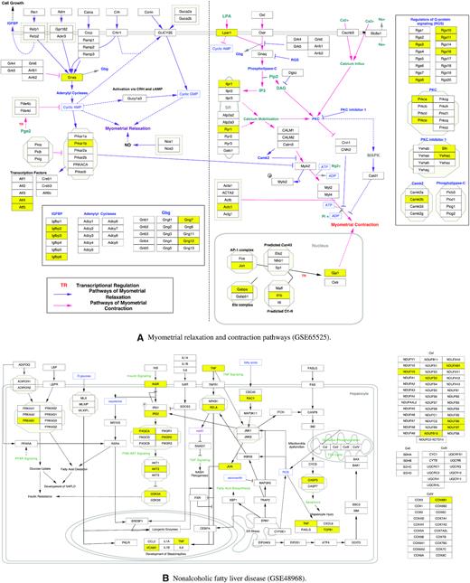
WikiPathways found from the central hidden layers trained on GSE65525, GSE48968, GSE52529, and GSE62270. (A) Myometrial relaxation and contraction pathways found in GSE65525. (B) Nonalcoholic fatty liver disease found in GSE48968. (C) VEGFA-VEGFR2 signaling pathway found in GSE52529. (D) Translation factors pathway found in GSE62270. In each pathway, the rectangle boxes represent the genes involved in the pathways, while the yellow boxes represent the genes corresponded to the central hidden layer.

DISCUSSION

In this study, we proposed a deep neural network framework, termed as DeepAE, to identify the key dimensions from high-dimensional biomolecular data (i.e. single-cell RNA-seq data, metabolic profiling data, and mass cytometry data). DeepAE is composed of an input layer, seven hidden layers, and output layer to form the encoder and decoder phases that are corresponded to the compression and decompression via three hidden layers, consistent with the three-layer cell regulation architecture revealed in the ENCODE project (50).

In compression, the encoder phase compresses the gene expression data without any restriction, in contrast to the linear limitation of CS-SMAF published on Cell; DeepAE can keep the non-linear patterns of the high-dimensional gene expression for key dimension identifications. Multiple experiments were conducted on nine single-cell transcriptomic datasets to compare the proposed DeepAE with the state-of-the-arts benchmark methods including SVD, k-SVD, sNMF, and CS-SMAF. The comparative results demonstrated that DeepAE outperforms other benchmark methods even when the compression level (measurements) is dropped from 100 to 10 key dimensions. Moreover, the recovery errors of DeepAE are significantly lower than the benchmark methods; it implies that DeepAE can recover the gene expression patterns in a quantitatively accurate manner.

In addition, we also investigate the performance of DeepAE in other biotechnologies such as mass cytometry and metabolic profiling. The mass cytometry data and metabolic profiling data are also stranded by high dimensionality and data sparsity issues. The experimental results demonstrated the performance of the proposed DeepAE as a general framework for uncovering key dimensions from high-throughput biomolecular data.

Moreover, we conducted a key dimension analysis on the central hidden layer of DeepAE to understand the biological meaning of each compressed key dimension. The visualization results from the original high-dimensional data and compressed data across all samples show that the the compressed data have still preserved the main topological patterns of the original data. We also investigated the biological meaning of each dimension of the central hidden layer through the GO enrichment analysis and pathology studies. It explains why and how the DeepAE model can capture key insights from the high-throughput biomolecular data of interest.

In the future, we hope that our DeepAE model can serve as a general platform for identifying the molecular drivers behind high-throughput biomolecular data with broad impacts on multiple directions such as cancer driver gene identification and stem cell lineage tracing.

SUPPLEMENTARY DATA

Supplementary Data are available at NAR Online.

ACKNOWLEDGEMENTS

The authors would also like to thank the three anonymous reviewers for their constructive comments.

FUNDING

Research Grants Council of the Hong Kong Special Administrative Region [CityU 11203217, CityU 11200218, CityU 21200816]; Health and Medical Research Fund; Food and Health Bureau of the Government of the Hong Kong Special Administrative Region [07181426]; Hong Kong Institute for Data Science (HKIDS) at City University of Hong Kong; City University of Hong Kong [CityU 11202219, in part]; National Natural Science Foundation of China [61603087]; Natural Science Foundation of Jilin Province [20190103006JH]; Fundamental Research Funds for the Central Universities [JGPY201902]. Funding for open access charge: Research Grants Council of the Hong Kong Special Administrative Region [CityU 11203217, CityU 11200218].

Conflict of interest statement. None declared.