


Abstract
Idealized equilibrium models have attributed the observed size structure of marine communities to the interactions between nutrient and grazing control. Here, we examine this theory in a more realistic context using a size-structured global ocean food-web model, together with a much simplified version of the same model for which equilibrium solutions are readily obtained. Both models include the same basic assumptions: allometric scaling of physiological traits and size-selective zooplankton grazing. According to the equilibrium model, grazing places a limit on the phytoplankton biomass within each size-class, while the supply rate of essential nutrients limits the number of coexisting size classes, and hence the total biomass, in the system. The global model remains highly consistent with this conceptual view in the large-scale, annual average sense, but reveals more complex behaviour at shorter timescales, when phytoplankton and zooplankton growth may become decoupled. In particular, we show temporal and spatial scale dependence between total phytoplankton biomass and two key ecosystem properties: the zooplankton-to-phytoplankton ratio, and the partitioning of biomass among different size classes.
INTRODUCTION
Marine phytoplankton communities are composed of a broad diversity of taxonomic groups that are often associated with distinct biogeochemical roles (Le Quéré et al., 2005). At the same time, these communities are clearly organized in terms of organism size, in a way that is thought to strongly influence the biologically mediated partitioning of carbon between the atmosphere and the ocean (Falkowski and Oliver, 2007). Ecosystem size structure and biodiversity are both important factors determining the biogeochemical function of marine systems, and there is a need to develop global models of ocean circulation, ecology and biogeochemistry that incorporate both these aspects, as we seek to improve our understanding of how systems function at the moment, and how they might respond to future environmental change.
A clear picture of the size structure in phytoplankton communities began to emerge in the 1980s, after several studies (Herbland and Le Boutier, 1981; Platt et al., 1983; Smith et al., 1985; Chavez, 1989) noted that the relative fraction of small cells tended to decrease with total chlorophyll a biomass. The observed chlorophyll a biomass in cells smaller than 1 µm in diameter was never greater than ∼0.5 mg chl a m−3, regardless of the total chlorophyll a biomass (Chisholm, 1992), with similar limits applying to larger size classes (Raimbault et al., 1988). This prompted Chisholm (Chisholm, 1992) to note that empirically “the total amount of chlorophyll in each size fraction has an upper limit”, and “thus, beyond certain thresholds, chlorophyll can only be added to the system by adding a larger size class”. Similar size structuring has also been observed in high-nitrate, low-chlorophyll (HNLC) regions, such as the equatorial Pacific and Southern Ocean, where low phytoplankton biomass has typically been associated with exclusion of large cells (Barber and Hiscock, 2006). In a recent review of size-fractionated chlorophyll a measurements, Marañón et al. (Marañón et al., 2012) demonstrated the ubiquity of this size-class partitioning across a range of marine environments, from the polar to the tropical.
These patterns have previously been explained using idealized equilibrium models, in terms of the balance between size-dependent nutrient uptake traits and density-dependent mortality (Thingstad and Sakshaug, 1990; Armstrong, 1994). In both nitrogen- and iron-limited systems, “top–down”, grazer or viral controls limit the amount of biomass within any particular size class, while the degree of “bottom–up” nutrient limitation dictates the number of size classes that can coexist, which in turn regulates the total biomass in the system. Planktonic marine ecosystems can thus be summarized as grazer controlled phytoplankton populations in nutrient-limited systems (Price et al., 1994).
This conceptual view suggests that community zooplankton:phytoplankton (Z:P) ratios should generally increase with total biomass, as a greater fraction of the community is brought under top–down control (Ward et al., 2012). This prediction is however at odds with results from a meta-analysis, where collated observations of open ocean and coastal plankton communities showed a negative correlation between phytoplankton biomass and total Z:P ratios (Gasol et al., 1997). Another apparently contradictory result is that iron fertilization experiments have been shown to stimulate growth in all phytoplankton size classes, not just in the largest and potentially most iron-limited groups (Kolber et al., 1994; Hiscock et al., 2008). Similarly, in iron-replete systems, blooms stimulated by shoaling of the mixed layer, or entrainment of nitrogen rich waters, often show dramatic growth of small as well as large species (Taylor et al., 1993; Barton et al., 2013). These observations appear contrary to the suggestion that total biomass accumulates through the progressive establishment of larger zooplankton and phytoplankton size classes (Armstrong, 1994).
In this article we will explore the conceptual balance of bottom–up nutrient supply and top–down grazing losses. We will use a combination of in situ observations, idealized theory (Armstrong, 1994; Poulin and Franks, 2010) and a global size-structured plankton food-web model (Ward et al., 2012), looking at both equilibrium and dynamic environments.
We first present direct observations highlighting the clear size structure of phytoplankton communities at the global scale. Following this, we describe a complex plankton food-web model that is able to reproduce this structure. We will outline a highly simplified version of this model that can be solved at equilibrium to help explain the behaviour of the more complex model. Having described the theory, we will examine the output from the size-structured global ecosystem model and show that the consistency of theory, model and observations provides support for the idea that marine communities are structured according to the size-dependent balance between nutrient acquisition and losses to grazing. In the Discussion section we will examine how the model behaviour differs dramatically from the equilibrium view on seasonal timescales, while at the same time remaining consistent with the theoretical view in terms of the annual average global trends.
OBSERVATIONS
The pattern of increasing phytoplankton biomass through the addition of larger size classes has been confirmed with large-scale field measurements in the Atlantic (Cavender-Bares et al., 2001; Marañón et al., 2001), and has also been inferred through the synthesis of in situ and remote observations (Uitz et al., 2006; Kostadinov et al., 2009; Hirata et al., 2011). Here we examine the phytoplankton size distribution using direct in situ observations from a wide range of sites. Approximately half the data come from a global compilation of size-fractionated chlorophyll a measurements, including Atlantic Meridional Transect (AMT) cruises 2 and 3 (Marañón et al., 2012), with the remainder taken from AMT cruises 6, 8, 10 and 11. This gives a total of 941 depth-resolved samples covering a wide range of environmental conditions.
Relationships between total and size-fractionated chlorophyll a concentrations are presented in Fig. 1a–c. Picophytoplankton (diameter <2 µm) are present across the full range of total chlorophyll a concentrations (Fig. 1a), and tend to dominate the biomass in systems with very low total chlorophyll a, where much larger phytoplankton are extremely rare. Picophytoplankton make up a smaller fraction of the total biomass at higher total chlorophyll a concentrations, reaching a maximum of approximately 0.5 ± 0.4 mg chl a m−3. Nanophytoplankton (diameter 2–20 µm) are relatively scarce at the lowest total chlorophyll a concentrations, but contribute a greater fraction of the total biomass at higher total chlorophyll a concentrations (Fig. 1b). Microphytoplankton (diameter >20 µm) are the least well represented size-class at very low chlorophyll a concentrations, but become relatively more important as total chlorophyll a exceeds 1 mg chl a m−3, becoming the dominant size-class at high total chlorophyll a concentrations (Fig. 1c). The axes are truncated at 2 mg chl a m−3 (excluding <6% of the observations), but we note that communities with total biomass greater than 2 mg chl a m−3 are also dominated by the microphytoplankton (see Marañón et al., 2012).
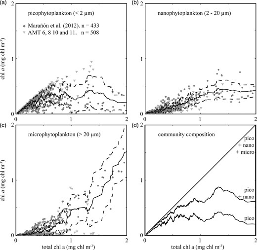
Chlorophyll a size fractionation. The grey dots in panels (a–c) indicate individual measurements from Marañón et al. (Marañón et al., 2012), triangles indicate data from AMT cruises 6, 8, 10 and 11. The bold lines show 20 point running means for picophytoplankton, nanophytoplankton and microphytoplankton chlorophyll a biomass ± 1 standard deviation (dashed lines) against total chlorophyll a biomass. Panel (d) shows the running means in each size-class plotted cumulatively on the y-axis, so that the chlorophyll a biomass in each size-class is represented by the vertical distance between lines.
This analysis confirms the size structure of phytoplankton communities a global scale, but what underpins the clear size structure seen in Fig. 1? In the following sections we will use a combination of a complex model and a simplified theory to explain how biomass accumulates through the progressive accumulation of larger and larger size-classes.
MODELS
We examine plankton community size structure using two ecosystem models of very different complexity: a full three-dimensional global ocean food-web model (Ward et al., 2012) based on the quota model of phytoplankton growth (Caperon, 1968; Droop, 1968; Geider et al., 1998), and a much simpler zero-dimensional, equilibrium approximation of the full model that uses the Monod (Monod, 1950) model of microbial growth. Because equilibrium solutions to the simpler model are relatively straightforward, its behaviour can be clearly understood. On the other hand, the more complex model is less abstract, and can be used to explore the behaviour of plankton communities in more detail and under more realistic (i.e. non-equilibrium) conditions.
A global ocean plankton food-web model
The “global food-web model” (Ward et al., 2012) resolves a complex food-web of 55 different phytoplankton and zooplankton types across a broad range of size-classes (a simplified schematic, reproduced from Ward et al. (Ward et al., 2012), is shown in Fig. 2a). This structure incorporates the two key assumptions that underpin the size structure of marine communities: first, the smallest cells have the highest affinity for nutrients, and second, each phytoplankton size-class is grazed by a limited number of zooplankton classes (Ward et al., 2012). Each size-class has double the volume of the previous size-class, so the 25 phytoplankton size-classes have diameter Ø1 = 0.6 µm ESD,  , while the 30 zooplankton size-classes have diameter Ø1 = 2.5 µm ESD,
  .
.
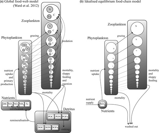
Schematic diagram describing (a) the global food-web model (reproduced from Ward et al., 2012), and (b) the idealized food-chain model.
Phytoplankton traits are assigned primarily on the basis of cell size, as described in Tables I and II (see also Ward et al., 2012), but there are four taxonomic groups that are additionally differentiated in terms of the maximum achievable photosynthetic rate at any given size (Table I). Within each taxonomic group the maximum photosynthetic rate decreases with increasing cell size, but for any given size diatoms are able to achieve the highest rates while Prochlorococcus are the slowest (Tang, 1995; Irwin et al., 2006; Ward et al., 2012). Because of this, the very small prokaryotes do not attain the unrealistically high photosynthetic rates that are predicted by a single allometric relationship for all taxa.
Size-dependent parameters in the global food-web model
| Parameter | Symbol | a | b | Parameter units |
|---|---|---|---|---|
| Maximum photosynthetic rate |  | 3.8 | −0.15 | day−1 |
 | 2.1 | −0.15 | day−1 | |
 | 1.4 | −0.15 | day−1 | |
 | 1.0 | −0.15 | day−1 | |
| Maximum uptake rate |  | 0.51 | −0.27 | mmol N (mmol C)−1 day−1 |
 | 0.51 | −0.27 | mmol N (mmol C)−1 day−1 | |
 | 0.26 | −0.27 | mmol N (mmol C)−1 day−1 | |
 | 1.4 × 10⁻⁶ | −0.27 | mmol Fe (mmol C)−1 day−1 | |
| Half-saturation for uptake |  | 0.17 | 0.27 | mmol N m−3 |
 | 0.17 | 0.27 | mmol N m−3 | |
 | 0.085 | 0.27 | mmol N m−3 | |
 | 80 × 10−6 | 0.27 | mmol Fe m−3 | |
| Phytoplankton min. N quota |  | 0.07 | −0.17 | mmol N (mmol C)−1 |
| Phytoplankton max. N quota |  | 0.25 | −0.13 | mmol N (mmol C)−1 |
| Maximum prey capture rate |  | 21.9 | −0.16 | day−1 |
| Phytoplankton sinking rate |  | 0.28 | 0.39 | m day−1 |
| Parameter | Symbol | a | b | Parameter units |
|---|---|---|---|---|
| Maximum photosynthetic rate | | 3.8 | −0.15 | day−1 |
| 2.1 | −0.15 | day−1 | |
| 1.4 | −0.15 | day−1 | |
| 1.0 | −0.15 | day−1 | |
| Maximum uptake rate | | 0.51 | −0.27 | mmol N (mmol C)−1 day−1 |
| 0.51 | −0.27 | mmol N (mmol C)−1 day−1 | |
| 0.26 | −0.27 | mmol N (mmol C)−1 day−1 | |
| 1.4 × 10⁻⁶ | −0.27 | mmol Fe (mmol C)−1 day−1 | |
| Half-saturation for uptake | | 0.17 | 0.27 | mmol N m−3 |
| 0.17 | 0.27 | mmol N m−3 | |
| 0.085 | 0.27 | mmol N m−3 | |
| 80 × 10−6 | 0.27 | mmol Fe m−3 | |
| Phytoplankton min. N quota | | 0.07 | −0.17 | mmol N (mmol C)−1 |
| Phytoplankton max. N quota | | 0.25 | −0.13 | mmol N (mmol C)−1 |
| Maximum prey capture rate | | 21.9 | −0.16 | day−1 |
| Phytoplankton sinking rate | | 0.28 | 0.39 | m day−1 |
For an organism with cell volume V (µm3), the parameter value is given by  (Ward et al., 2012).
Size-dependent parameters in the global food-web model
| Parameter | Symbol | a | b | Parameter units |
|---|---|---|---|---|
| Maximum photosynthetic rate | | 3.8 | −0.15 | day−1 |
| 2.1 | −0.15 | day−1 | |
| 1.4 | −0.15 | day−1 | |
| 1.0 | −0.15 | day−1 | |
| Maximum uptake rate | | 0.51 | −0.27 | mmol N (mmol C)−1 day−1 |
| 0.51 | −0.27 | mmol N (mmol C)−1 day−1 | |
| 0.26 | −0.27 | mmol N (mmol C)−1 day−1 | |
| 1.4 × 10⁻⁶ | −0.27 | mmol Fe (mmol C)−1 day−1 | |
| Half-saturation for uptake | | 0.17 | 0.27 | mmol N m−3 |
| 0.17 | 0.27 | mmol N m−3 | |
| 0.085 | 0.27 | mmol N m−3 | |
| 80 × 10−6 | 0.27 | mmol Fe m−3 | |
| Phytoplankton min. N quota | | 0.07 | −0.17 | mmol N (mmol C)−1 |
| Phytoplankton max. N quota | | 0.25 | −0.13 | mmol N (mmol C)−1 |
| Maximum prey capture rate | | 21.9 | −0.16 | day−1 |
| Phytoplankton sinking rate | | 0.28 | 0.39 | m day−1 |
For an organism with cell volume V (µm3), the parameter value is given by (Ward et al., 2012).
A number of other physiological traits also scale with cell size, as outlined in Table I. Both the minimum and maximum nitrogen quotas increase with size, with the maximum quota increasing at a faster rate, such that larger cells have a greater capacity to store excess nitrogen, relative to their requirements for growth (Montagnes and Franklin, 2001). Zooplankton grazing rates tend to increase with decreasing organism size (Hansen et al., 1997), which leads to stronger grazing pressure on the smallest phytoplankton size-classes.
The time-dependent change in the biomass of each of the modelled plankton types is described in terms of growth, sinking, grazing and other mortality, as well as physical transport and mixing. Phytoplankton growth is a light- and temperature-dependent function of intracellular nutrient reserves (Droop, 1968; Geider et al., 1998). Inorganic nutrients are taken up by phytoplankton and are subsequently transformed into organic matter. Sloppy feeding and mortality transfer living organic material into sinking particulate and dissolved organic detritus which is respired back to inorganic form. Iron chemistry includes explicit complexation with an organic ligand, scavenging by particles (Parekh et al., 2005) and representation of aeolian (Luo et al., 2008) and sedimentary (Elrod et al., 2004) sources. The ecosystem model is embedded within a global model of ocean circulation (MITgcm; Marshall et al., 1997) that has been constrained with satellite and hydrographic observations (Estimation of the Circulation and Climate of the Ocean (ECCO); Wunsch and Heimbach, 2007). A complete description of the model formulation is given in Ward et al. (Ward et al., 2012).
A simplified zero-dimensional equilibrium approximation of the full model
The global food-web model includes a relatively high degree of ecological and physiological complexity and is embedded within a spatially and temporally heterogeneous representation of the physical environment. This complexity allows better comparison with observations and more detailed predictions, but can also make the model behaviour difficult to understand.
With this in mind, we also consider a highly simplified version of the model that can be solved for equilibrium. In this “idealized food-chain model” the physical environment is reduced to a zero-dimensional chemostat. Nutrient medium of concentration ( ) is fed in according to the dilution rate κ, while phytoplankton (P) and nitrate (N) are washed out at the same rate. Zooplankton (Z) are assumed to maintain themselves in the chemostat (and they do not sink in the global model). The idealized model has the same phytoplankton size-classes as the global food-web model, but there are only 25 grazers because each phytoplankton size-class is grazed by only one zooplankton size-class (1024 times larger by volume) and the zooplankton have no grazers. A simplified schematic is given in Fig. 2b.
 ) and does not include iron limitation. It is based on the Monod (Monod, 1950) model of phytoplankton growth, such that nutrient uptake and growth are always balanced. Dissolved nitrogen (N) is consumed by each phytoplankton size-class (
 ) as a saturating function of N, where
  is the maximum growth rate (day−1) and
  is the half-saturation concentration (mmol N m−3). Light and temperature limitation are also included through a dimensionless parameter, γ. Zooplankton size classes (
 ) each graze only one size class of phytoplankton according to a non-saturating clearance rate,
  (m3 day−1 (mmol N)−1). Grazed biomass is assimilated with efficiency λ. Phytoplankton and zooplankton are each subject to a linear mortality term, which is labelled m (day−1) for phytoplankton and δ (day−1) for zooplankton. All dead and unassimilated matter is exported from the system. N, P and Z are measured in units of nitrogen (mmol N m−3).
Parameterization
Verdy et al. (Verdy et al., 2009) showed that when nutrient uptake and growth are balanced, the quota model of phytoplankton growth (Caperon, 1968; Droop, 1968) can be approximated by the Monod (Monod, 1950) model, where the maximum growth rate and half-saturation constant are functions of the quota model parameters. Here we use equations 12 and 13 of Verdy et al. (Verdy et al., 2009) to parameterize the idealized food-chain model (Table II) in terms of the parameters of the full global food-web model (Tables I and III). This approximation leads to size-dependent growth parameters for the two models that are consistent with each other. The size-dependent traits for the idealized food-chain model are shown in Fig. 3.
Size-independent parameters in the global food-web model (Ward et al., 2012)
| Parameter | Symbol | Value | Units |
|---|---|---|---|
| Ammonium inhibition parameter | ψ | 4.6 | (mmol N m−3)−1 |
| Zooplankton minimum N quota |  | 0.075 | mmol N (mmol C)−1 |
| Zooplankton maximum N quota |  | 0.151 | mmol N (mmol C)−1 |
| Plankton minimum Fe quota |  | 1.5 × 10⁻⁶ | mmol Fe (mmol C)−1 |
| Plankton maximum Fe quota |  | 80 × 10−6 | mmol Fe (mmol C)−1 |
| Reference temperature |  | 20 | °C |
| Temperature dependence | R | 0.05 | – |
| Maximum Chl-a-to-N ratio |  | 3.0 | mg Chl a (mmol N)−1 |
| Initial slope of P–I curve |  | 3.83 × 10⁻⁷ | mmol C (mg Chl a)−1 (µEin m−2)−1 |
| Cost of biosynthesis | ξ | 2.33 | mmol C (mmol N)−1 |
| Optimal predator-to-prey length ratio |  | 10* | – |
Standard deviation of  |  | 0.5 | – |
| Total prey half-saturation |  | 1 | mmol C m−3 |
| Maximum assimilation efficiency |  | 0.7 | – |
| Prey refuge parameter | λ | −1 | – |
| Background mortality |  | 0.02 | day−1 |
| Fraction to DOM at death |  | 0.5 | – |
 | 0.8 | – | |
 to to  oxidation rate oxidation rate |  | 2 | day−1 |
 to to  oxidation rate oxidation rate |  | 0.1 | day−1 |
| PAR threshold for nitrification |  | 10 | µEin m−2 s−1 |
| Iron scavenging rate |  | 4.4 × 10⁻³ | day−1 |
| DOM remineralisation rate |  | 0.02 | day−1 |
| POM remineralisation rate |  | 0.04 | day−1 |
| DOM sinking rate |  | 0 | m day−1 |
| POM sinking rate |  | 10 | m day−1 |
| Light attenuation by water |  | 0.04 | m−1 |
| Light attenuation by Chl a |  | 0.03 | m−1 (mg Chl a)−1 |
| Parameter | Symbol | Value | Units |
|---|---|---|---|
| Ammonium inhibition parameter | ψ | 4.6 | (mmol N m−3)−1 |
| Zooplankton minimum N quota | | 0.075 | mmol N (mmol C)−1 |
| Zooplankton maximum N quota | | 0.151 | mmol N (mmol C)−1 |
| Plankton minimum Fe quota | | 1.5 × 10⁻⁶ | mmol Fe (mmol C)−1 |
| Plankton maximum Fe quota | | 80 × 10−6 | mmol Fe (mmol C)−1 |
| Reference temperature | | 20 | °C |
| Temperature dependence | R | 0.05 | – |
| Maximum Chl-a-to-N ratio | | 3.0 | mg Chl a (mmol N)−1 |
| Initial slope of P–I curve | | 3.83 × 10⁻⁷ | mmol C (mg Chl a)−1 (µEin m−2)−1 |
| Cost of biosynthesis | ξ | 2.33 | mmol C (mmol N)−1 |
| Optimal predator-to-prey length ratio | | 10* | – |
| Standard deviation of | | 0.5 | – |
| Total prey half-saturation | | 1 | mmol C m−3 |
| Maximum assimilation efficiency | | 0.7 | – |
| Prey refuge parameter | λ | −1 | – |
| Background mortality | | 0.02 | day−1 |
| Fraction to DOM at death | | 0.5 | – |
| 0.8 | – | |
| to oxidation rate | | 2 | day−1 |
| to oxidation rate | | 0.1 | day−1 |
| PAR threshold for nitrification | | 10 | µEin m−2 s−1 |
| Iron scavenging rate | | 4.4 × 10⁻³ | day−1 |
| DOM remineralisation rate | | 0.02 | day−1 |
| POM remineralisation rate | | 0.04 | day−1 |
| DOM sinking rate | | 0 | m day−1 |
| POM sinking rate | | 10 | m day−1 |
| Light attenuation by water | | 0.04 | m−1 |
| Light attenuation by Chl a | | 0.03 | m−1 (mg Chl a)−1 |
Size-independent parameters in the global food-web model (Ward et al., 2012)
| Parameter | Symbol | Value | Units |
|---|---|---|---|
| Ammonium inhibition parameter | ψ | 4.6 | (mmol N m−3)−1 |
| Zooplankton minimum N quota | | 0.075 | mmol N (mmol C)−1 |
| Zooplankton maximum N quota | | 0.151 | mmol N (mmol C)−1 |
| Plankton minimum Fe quota | | 1.5 × 10⁻⁶ | mmol Fe (mmol C)−1 |
| Plankton maximum Fe quota | | 80 × 10−6 | mmol Fe (mmol C)−1 |
| Reference temperature | | 20 | °C |
| Temperature dependence | R | 0.05 | – |
| Maximum Chl-a-to-N ratio | | 3.0 | mg Chl a (mmol N)−1 |
| Initial slope of P–I curve | | 3.83 × 10⁻⁷ | mmol C (mg Chl a)−1 (µEin m−2)−1 |
| Cost of biosynthesis | ξ | 2.33 | mmol C (mmol N)−1 |
| Optimal predator-to-prey length ratio | | 10* | – |
| Standard deviation of | | 0.5 | – |
| Total prey half-saturation | | 1 | mmol C m−3 |
| Maximum assimilation efficiency | | 0.7 | – |
| Prey refuge parameter | λ | −1 | – |
| Background mortality | | 0.02 | day−1 |
| Fraction to DOM at death | | 0.5 | – |
| 0.8 | – | |
| to oxidation rate | | 2 | day−1 |
| to oxidation rate | | 0.1 | day−1 |
| PAR threshold for nitrification | | 10 | µEin m−2 s−1 |
| Iron scavenging rate | | 4.4 × 10⁻³ | day−1 |
| DOM remineralisation rate | | 0.02 | day−1 |
| POM remineralisation rate | | 0.04 | day−1 |
| DOM sinking rate | | 0 | m day−1 |
| POM sinking rate | | 10 | m day−1 |
| Light attenuation by water | | 0.04 | m−1 |
| Light attenuation by Chl a | | 0.03 | m−1 (mg Chl a)−1 |
Parameters for the idealized food-chain model
| Parameter | Symbol | Value or formula | Units |
|---|---|---|---|
| Deep N concentration |  | Variable (0–5) | mmol N m−3 |
| Chemostat mixing rate | κ | 0.01 | day−1 |
| Light and temperature limitation | γ | 0.1 | – |
| Maximum growth rate at 20°C |  |  | day−1 |
| Half-saturation for growth |  |  | mmol N m−3 |
| Nutrient affinity | α |  | m3 day−1 (mmol N)−1 |
| Grazing clearance rate | g |  V−0.16 V−0.16 | m3 day−1 (mmol N)−1 |
| Assimilation efficiency | λ | 0.7 | – |
| Phytoplankton mortality | m | 0.02 | day−1 |
| Zooplankton mortality | δ | 0.05V−0.16 | day−1 |
| Parameter | Symbol | Value or formula | Units |
|---|---|---|---|
| Deep N concentration | | Variable (0–5) | mmol N m−3 |
| Chemostat mixing rate | κ | 0.01 | day−1 |
| Light and temperature limitation | γ | 0.1 | – |
| Maximum growth rate at 20°C | | | day−1 |
| Half-saturation for growth | | | mmol N m−3 |
| Nutrient affinity | α | | m3 day−1 (mmol N)−1 |
| Grazing clearance rate | g | V−0.16 | m3 day−1 (mmol N)−1 |
| Assimilation efficiency | λ | 0.7 | – |
| Phytoplankton mortality | m | 0.02 | day−1 |
| Zooplankton mortality | δ | 0.05V−0.16 | day−1 |
The Monod parameters  and
and  are set according to the parameters of the quota model, using the conversion factors given by Verdy et al. (Verdy et al., 2009). Here
  and μ∞ = PCmax. The non-saturating grazing clearance rate is given by the ratio of the maximum grazing rate and half-saturation constant from the full model, converting to nitrogen units. λ and m are as for the full model, but δ is made size-dependent for reasons described in the main text.
Parameters for the idealized food-chain model
| Parameter | Symbol | Value or formula | Units |
|---|---|---|---|
| Deep N concentration | | Variable (0–5) | mmol N m−3 |
| Chemostat mixing rate | κ | 0.01 | day−1 |
| Light and temperature limitation | γ | 0.1 | – |
| Maximum growth rate at 20°C | | | day−1 |
| Half-saturation for growth | | | mmol N m−3 |
| Nutrient affinity | α | | m3 day−1 (mmol N)−1 |
| Grazing clearance rate | g | V−0.16 | m3 day−1 (mmol N)−1 |
| Assimilation efficiency | λ | 0.7 | – |
| Phytoplankton mortality | m | 0.02 | day−1 |
| Zooplankton mortality | δ | 0.05V−0.16 | day−1 |
The Monod parameters and are set according to the parameters of the quota model, using the conversion factors given by Verdy et al. (Verdy et al., 2009). Here and μ∞ = PCmax. The non-saturating grazing clearance rate is given by the ratio of the maximum grazing rate and half-saturation constant from the full model, converting to nitrogen units. λ and m are as for the full model, but δ is made size-dependent for reasons described in the main text.
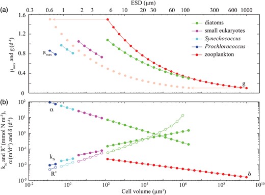
Size-dependent physiological parameters for the idealized food-chain model. The light pink dots in (a) show the zooplankton grazing rates shifted along the x-axis for comparison to the maximum growth rates of their phytoplankton prey.
Some modifications were required to bring the behaviour of the idealized equilibrium model closer to that of the global food-web model. In particular, the light and temperature limitation parameter, γ, was set to 0.1. This allows greater coexistence of larger size–classes because it increases the sensitivity of phytoplankton competitive ability to zooplankton grazing [see equation (4)]. Additionally, the zooplankton size-dependent mortality rate, δ, was made size-dependent to account for the omission of carnivorous grazing on zooplankton. This parameterisation flattens the phytoplankton biomass distribution by providing a refuge for smaller phytoplankton size classes and preventing the unrealistic accumulation of larger groups (Poulin and Franks, 2010).
RESULTS
We first analyse the idealized equilibrium model and will later go on to compare its behaviour with that of the full global food-web model.
Equilibrium solutions to the idealized food-chain model
 at which phytoplankton size-class
  can exist at steady state is given by
 is thus a function of its maximum growth rate, nutrient half-saturation constant, combined losses from mortality and dilution, as well as the level of grazing pressure, given by the product of the grazing rate and the biomass of the paired zooplankton predator. Setting
  to zero gives the absolute minimum nitrogen concentration required for survival of plankton size-class i in the absence of its paired grazer.
 increasing with size (Fig. 3). In a similar fashion, the minimum phytoplankton biomass
  required to support
  at equilibrium is given by,
 has become established, the biomass of phytoplankton
  is cropped to a constant value that is a function of the zooplankton grazing rate, assimilation efficiency and mortality rate. Finally, the size of the zooplankton population at equilibrium is given by,
This equation states that zooplankton class  will reach its peak biomass once its prey are growing at their maximum, saturated rate (i.e. when
  ).
).
Community size–structure in the idealized food-chain model
The idealized food-chain model is examined at steady-state across a range of incoming nutrient concentrations,  . With the dilution rate κ held fixed, increasing
  corresponds to an increasing nutrient supply rate. At each concentration the model was integrated forwards with parameter values as defined in Table III, until an equilibrium was reached.
The equilibrium relationship between total biomass and size-fractionation is shown across a range of increasing  in Fig. 4a. Beginning at the left-hand side of this plot, the incoming nutrient concentration
  is initially less than the critical value (
 ) that is required to support even the smallest phytoplankton size-class. However, once
  exceeds
  , the first phytoplankton size-class
  becomes established and N is drawn down to
  ; any excess nitrogen is passed directly into phytoplankton biomass. The biomass of
  will initially be too small to support its zooplankton grazer (
 ), but once phytoplankton biomass reaches the threshold value (
 ),
),  will become viable and this newly established population will crop
  to
to  .
.
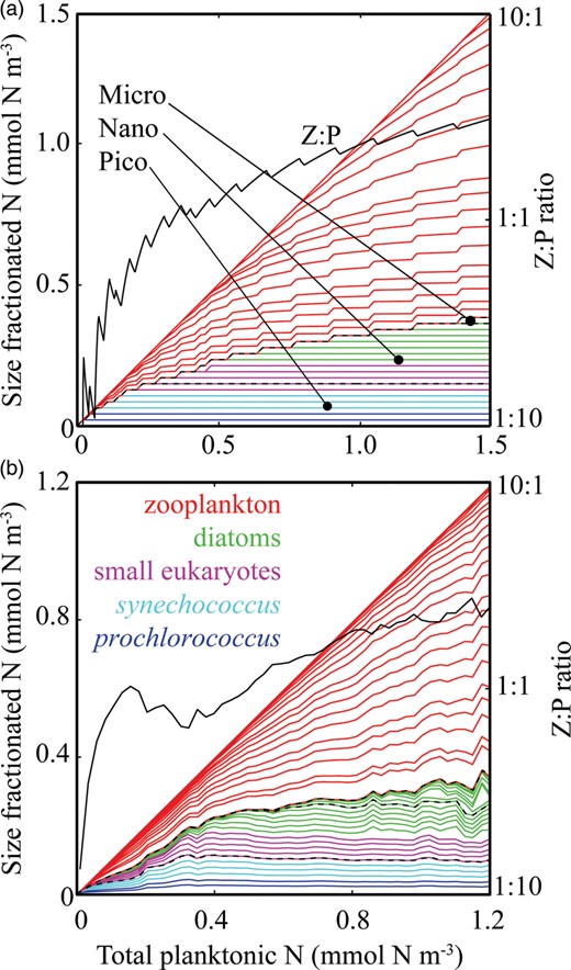
Community size structure with increasing total plankton biomass in (a) the idealized food-chain model and (b) the global food-web model. For both panels, biomass in each size-class is presented cumulatively, and distances between the lines indicate individual phytoplankton and zooplankton biomasses. The uppermost line in each group represents total phytoplankton and zooplankton biomass. Colours correspond to the plankton taxa (see legend), while dotted black lines represent the biomass in pico-, nano- and microphytoplankton. Equilibrium Z:P ratios are shown with a black line corresponding to the right-hand axis (log scale). Global model biomass data are annual mean values for the surface layer, within 50 equally spaced bins of total phytoplankton and zooplankton biomass.
As  is increased further, phytoplankton population
  grows faster, but strong top–down control from
  means any extra growth is passed directly into zooplankton biomass. With increased mortality from grazing,
  will no longer be able to draw nutrients down to the same low-level as before, and inorganic N will accumulate. Eventually, N will increase to
  , at which point the next phytoplankton class,
  , will become established.
With further increases in  , paired phytoplankton and zooplankton classes successively become established. The phytoplankton biomass within any single size-class is limited by grazing from the top–down, while the total biomass in the system is limited by nutrient supply from the bottom–up, as progressively less competitive size-classes become established with increasing nutrient availability. Increasing
  in this way is analogous to moving from low biomass, oligotrophic environments to high biomass and eutrophic environments.
With this progressive accumulation of paired phytoplankton and zooplankton size-classes, increasing total biomass is associated with increasing Z:P ratios. A low biomass system will be dominated by small, resource-limited phytoplankton with few grazers. Higher biomass systems have a Z:P ratio reflecting the large number of paired phytoplankton and zooplankton size-classes.
Community size–structure in the global food-web model
The equilibrium view described above provides a mechanistic explanation for the size–structure of marine communities (Armstrong, 1994; Poulin and Franks, 2010). The zero-dimensional, equilibrium approach is, however, highly simplified. Compared with the global food-web model, the idealized model ignores spatial and temporal variability, physical dispersal of plankton biomass, explicit quota physiology, multiple nitrogen species and iron limitation, size-dependent phytoplankton sinking, recycling of organic matter and greater food-web complexity.
In the following section we examine output from the global food-web model (Ward et al., 2012) to explore the relevance of this steady-state theory within a more realistic ecological and environmental framework [we note that simulated global distributions of annual mean nitrate, chlorophyll a and primary production are qualitatively consistent with observational estimates, and the biogeography of size-fractionated phytoplankton functional types match satellite derived estimates (Hirata et al., 2011; Ward et al., 2012)].
Figure 4b shows surface values of phytoplankton and zooplankton biomass from the global food-web model with increasing total surface biomass. The behaviour of the complex ecosystem model agrees well with results from the much simpler idealized model shown in Fig. 4a. With total plankton biomass increasing along the x-axis, the smallest phytoplankton size-classes have a relatively constant biomass from the most oligotrophic to the most eutrophic regions. Progressively larger size-classes become established with increasing total biomass. There is also a similar increase in community Z:P.
The close agreement between the complex and idealized models reflects the fact that they are both structured according to the same rules. In particular, fundamental physiological traits scale with organism size, and grazing by zooplankton is structured by an optimal predator–prey length ratio. If the specialist grazers in the global model are replaced by generalist zooplankton with no size preference, the size distribution and biodiversity collapse to just one dominant size-class at each location (see Ward et al., 2012). The results are also sensitive to smaller changes in the breadth of the optimal predator–prey size-preference kernel (Fuchs and Franks, 2010). Coexistence of all size-classes was only possible when the grazing size-preference kernel had a standard deviation no greater than 0.5 in log space. This is slightly narrower than some empirical estimates (Kiørboe, 2008), but it should be noted that the model does not include other potentially important density-dependent loss processes, such as viral lysis (Suttle, 1994; Thingstad, 2000) and aggregation mediated sinking (Burd and Jackson, 2008).
Spatial patterns in the global food-web model
The sizes of the largest phytoplankton and zooplankton size-class within each surface grid cell (as defined in the figure legend) are shown in Fig. 5. We switch our focus to carbon at this point because it is the dominant element in plankton dry biomass and it is assumed to provide a good indication of plankton numerical abundance (Menden-Deuer and Lessard, 2000). Consideration of carbon also removes any potential effects of excess uptake of non-limiting N or Fe (Geider and La Roche, 2002).
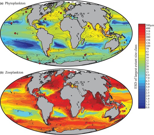
Global size and biomass distributions in the global food-web model for (a) phytoplankton and (b) zooplankton at the surface (0–10 m). The colour scale represents the equivalent spherical diameter of the largest extant plankton size-class within each surface grid cell. A plankton class is considered extant if its annual mean carbon biomass is >0.1% of total plankton carbon biomass (Barton et al., 2013). Contours show annual average total plankton carbon biomass (mmol C m−3). The location of nine JGOFS sites (see Figs 6–8) are shown with red dots in the upper panel: (a) HOT, (b) BATS, (c) Equatorial Pacific, (d) Arabian Sea, (e) NABE, (f) Station P, (g) Kerfix, (h) Polar Front, and (i) Ross Sea.
The largest size-classes are found in the North Atlantic, the North West Pacific, the Indian Ocean, around coastal upwelling zones, and downstream of landmasses in the Southern Ocean. Large cells are notably absent from the sub-tropical gyres and the three HNLC regions: the North East Pacific, the Equatorial Pacific and much of the Southern Ocean.
Figure 5 also shows the surface phytoplankton and zooplankton carbon biomass (contours). There is a close spatial agreement between the annual mean plankton biomass and the size of the largest organism. Total phytoplankton carbon biomass and  are correlated with r = 0.68, while total zooplankton carbon biomass and
  are correlated with r = 0.78.
DISCUSSION
Despite the complexity of the observed ocean, and of the three-dimensional ocean simulation (which resolves complex, non-equilibrium dynamics, internal cell physiology, organic matter and multiple limiting factors), the relatively simple theory appears to capture the observed large-scale, time-averaged organization. Observations, model and theory all consistently show that, in an annual average sense, regions of higher total plankton biomass support progressively larger size-classes. This pattern is driven by the high nutrient affinity of small cells, coupled to the regulating effects of size-specific grazing (Armstrong, 1994; Poulin and Franks, 2010). At steady-state, small cells have the potential to outcompete larger cells for limiting nutrients, but intense grazing pressure prevents any one size-class from dominating and allows larger phytoplankton types to coexist with the smaller cells. With increasing total phytoplankton biomass large phytoplankton do not replace smaller species, but instead coexist alongside them.
Z:P ratios
The idealized equilibrium model predicts that Z:P ratios increase with total phytoplankton biomass (Fig. 4 and Armstrong, 1994). This pattern is also evident in the annual averages of the global food-web model (Figs 4 and 5). In contrast, collated observations of both pelagic and coastal plankton communities have suggested that Z:P ratios are in fact negatively correlated with total phytoplankton biomass (Gasol et al., 1997). How can these two opposing views be reconciled?
While the global model suggests that P and Z:P are positively correlated in terms of the annual average (Fig. 4b), at each individual site the correlation is actually negative throughout the seasonal cycle (Fig. 6). During a phytoplankton bloom, Z:P initially decreases because phytoplankton biomass increases much more rapidly than the zooplankton population. Subsequently, Z:P increases as the zooplankton population peaks at the expense of the phytoplankton population. The Z:P ratio tends to decrease gradually after this, as both the zooplankton and phytoplankton populations decline.
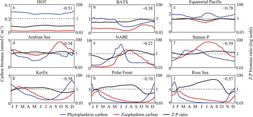
Surface phytoplankton and zooplankton carbon biomasses (blue and red lines) in the global food-web model at the nine JGOFS sites (red dots in Fig. 5). Total Z:P carbon biomass ratios are also shown (right-hand axes). The local correlation between P and Z:P is shown in the top left-hand corner of each subplot.
The difference between the daily resolved and annual average trends are explored in greater detail in Fig. 7. In each panel we show the best-fit relationship between P and Z:P under three different sampling strategies: (i) model data from all locations, (ii) model data from just the locations of the 9 Joint Global Ocean Flux Study (JGOFS) time series and process study sites, and (iii) model data from the JGOFS sites excluding the most oligotrophic site, the Hawaii ocean Time-series (HOT).
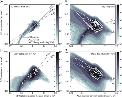
Relationship between P and Z:P in annual mean (a) and daily (b–d) output from the global food-web model. Panels (a) and (b) represent the global ocean, while (c) and (d) discriminate between low-latitude and high-latitude locations. Shading corresponds to the frequency density of data within each of 64 × 64 discrete bins. The white circles represent the modelled annual mean P to Z:P relationship at each of the nine JGOFS sites, while the white loops describe the relationship throughout the climatological model year. The grey lines represent the best-fit power-law relationship ( ) for all data (solid line), the JGOFS sites only (dashed line), and the JGOFS sites excluding the most oligotrophic site, HOT (dot-dashed line, panels a and b only).
In terms of the annual average, the P to Z:P relationships agree with the predictions of the equilibrium model, with positive slopes between 0.80 and 1.16 (Fig. 7a). However, the best-fit slopes were much more variable in the daily data, taking positive or negative values, between −0.54 and 0.31 (Fig. 7b).
If the daily resolved model results are split into low latitude (<40°) and high latitude (>40°) regions, a positive relationship can be seen between P and Z:P at low latitudes (0.94 to 1.45), switching to a negative relationship at higher latitudes (−0.66−0.48). The individual trajectories of P versus Z:P throughout the seasonal cycle (white lines) indicate that significant decoupling can occur at high latitudes, when individual zooplankton size-classes are slow to respond to the sudden growth of their phytoplankton prey. It is this decoupling that drives the negative correlations seen when the simulation is examined with daily resolution.
Although the annual mean slope of Z:P relative to P is always positive in the simulations (Fig. 7a), observed data (which are typically sparse in space and time) show the opposite trend (Gasol et al., 1997). Figure 7(c) and (d) show that this relationship can vary significantly during the course of events where growth and loss become decoupled, and that this behaviour may dominate the observed relationship if the sampling is incomplete (note the changes in slope with different sampling regimes in Fig. 7b). These results suggest that the observed negative relationship between P and Z:P may be a sampling issue, and we hypothesize that if a more comprehensive set of observations were available, the data would follow the predicted trend.
Phytoplankton blooms driven by growth in all size-classes: a rising tide lifts all boats?
Observations of both nitrogen- and iron-limited systems indicate that phytoplankton blooms are driven by growth of phytoplankton in all size-classes, not just in the largest size-classes (Barber and Hiscock, 2006). This could be viewed as contrary to the idea that biomass builds up through the addition of larger size-classes. If top–down controls really limit the amount of biomass within each size-class, how is it that nutrient addition or shoaling of the mixed layer leads to growth in all size-classes?
Figure 8A–I shows the seasonal cycle of modelled chlorophyll a, in comparison with observed chlorophyll a biomass for nine JGOFS time-series sites (Kleypas and Doney, 2001). The observations are composites of all years for which data were available, so include some interannual variability that could not be reproduced by the climatological model (Ward et al., 2012). Likewise, the coarse resolution of the ocean model precludes the reproduction of variability associated with the mesoscale and below. Nonetheless, the model tracks the general trends at all sites, with the exception of HOT, where the total chlorophyll a is underestimated by ∼0.05 mg chl a m−3 (Ward et al., 2012). Total modelled chlorophyll a in Fig. 8A–I is also broken down according to contributions from each phytoplankton size-class. At all sites, even the smallest size-classes show some seasonal variability, and growth of the total phytoplankton population is frequently driven by growth in all size-classes.
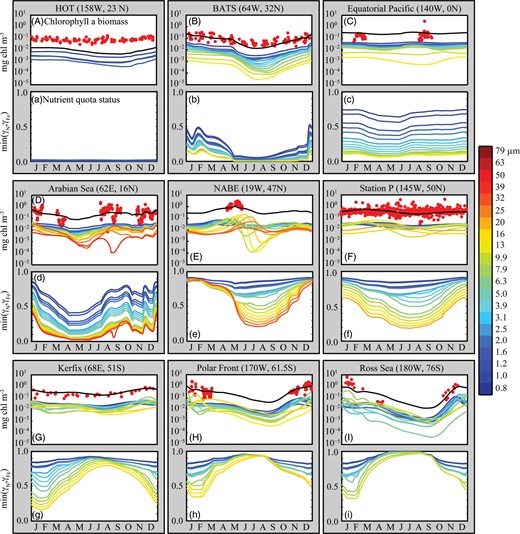
Panels (A–I): modelled mixed-layer total chlorophyll a concentrations (black lines) in the global food-web model, with in situ measurements from JGOFS sites (red dots). The site locations are indicated in Fig. 5. Chlorophyll a concentrations within individual model size-classes are also shown, with cell diameter represented by colour. Size-classes for which the surface biomass did not once exceed 0.001 mg chl a m−3 are excluded. Panels (a–i): the status of the most limiting quota (N or Fe) within each phytoplankton size-class (see main text for details).
Figure 8a–i shows the nutrient quota status,  , where for each phytoplankton class, j,
  is the quota nitrogen status and
  is the quota iron status (Ward et al., 2012). This gives an indication of the degree of nutrient limitation in each class (1 is completely nutrient replete, 0 is completely starved of either N or Fe). (The quota status term does not explicitly account for light or temperature limitation.)
Figure 8a–i demonstrates an important point which explains why phytoplankton blooms typically occur in all size-classes, including those under top–down control. It is important to note that when a phytoplankton size-class is under grazer control, this does not mean that the growth rate of that size-class is not at the same time limited from the bottom–up. It simply means that its growth rate (as a function of nutrient availability, light and temperature) is balanced by grazing pressure. Figure 8 demonstrates that all size-classes are in fact subject to some degree of nutrient limitation, and that this may vary substantially throughout the year (except perhaps at HOT). Nutrient injection will therefore lead to faster growth in a wide range of size-classes (Morel et al., 1991). Similarly, sudden relief of light limitation allows rapid nutrient uptake and growth in all size-classes.
A perturbation, such as increased light levels, or a nutrient pulse, will raise growth rates in all size-classes where growth is not already saturated. Wherever the increased growth is sufficient for a phytoplankton size-class to become decoupled from its zooplankton grazers, that size-class will bloom. Decoupling may be initiated by a number of mechanisms, most notably nutrient addition or increased light levels, but in any case, the overall bloom will be driven by growth in many, if not all size-classes.
After an initial lag, the grazer populations will respond, drawing phytoplankton populations back under grazer control. The rate of recoupling, and hence bloom termination in an individual size-class will depend on the difference between the rates of phytoplankton growth and zooplankton grazing, as shown in Fig. 3a. The smallest picophytoplankton do not contribute significantly to blooms because they grow relatively slowly, and are preferentially grazed by small zooplankton with high grazing rates; any decoupled growth can be brought rapidly back under grazing control. Intermediate-sized phytoplankton are able to dominate blooms because they have slower growing grazers, and may have faster growth rates, than very small cells. The size of the bloom in each size-class is thus dependent on the ratio of phytoplankton and zooplankton response time-scales (Franks, 2001). Intermediate and large phytoplankton tend to dominate blooms as they are able to remain decoupled from grazing for longer (Barber and Hiscock, 2006).
The complex model behaviour demonstrates the compatibility of both the equilibrium view (at large spatial scales in terms of the annual average) and the non-equilibrium view (locally, on time scales of weeks to months). Regardless of the non-equilibrium behaviour, the number of size-classes that are established at each location is positively correlated with the total biomass, suggesting that phytoplankton size plays a crucial role in regulating global plankton biogeography.
Resource competition in non-equilibrium environments
The equilibrium model suggests that community structure is dominated by two key processes. On the one hand, small cells are typically the best competitors for nutrients. On the other, density-dependent losses associated with grazing prevent the small cells from using all nutrients to the exclusion of other less competitive types. Nonetheless, in environments that are frequently perturbed from equilibrium, is the equilibrium model relevant at all? Is it likely that we are getting the “right” answer for the “wrong” reasons?
No marine environment can be accurately described as a true ecological equilibrium. Nutrients are injected at both regular and irregular intervals through a variety of physical disturbances, including mesoscale eddies, internal waves and convective overturning. These disturbances often lead to the accumulation of surface nutrients, particularly at high latitudes, where light and temperature prevent full nutrient drawdown during winter. When nutrients are abundant, community composition is less likely to be affected by competition for resources, and traits such as fast growth or the ability to withstand disturbance should become more important.
It has been suggested that larger cells may gain an advantage in temporally or spatially varying environments on account of having a higher ratio of maximum to minimum quota ( ) than smaller cells (Grover, 1991; Kerimoglu et al., 2012). With larger
  , cells may accumulate more of a limiting resource during periods of surplus, relative to their basal requirements; an advantage that may compensate for lower nutrient affinities during periods of resource competition (Grover, 1991; Litchman et al., 2009). This mechanism can be seen in Fig. 8e at the NABE location, where the nutrient status of the largest cells (orange colours) initially declines more slowly during the bloom than is seen for intermediate cells (green colours). Nonetheless, at this site, the period of nutrient limitation is long enough that the largest cells eventually suffer from the strongest nutrient limitation, on account of their less competitive nutrient uptake traits. Indeed, although
  increases with cell size in this study, in the absence of grazer controls, this mechanism was not enough to sustain cells larger than 2 µm ESD at any modelled location (Ward et al., 2012). These results are consistent with other modelling studies that have shown pulsed nutrient supplies with periods of several months were not able to prevent fast growing cells with modest
  from outcompeting slower growing cells with greater
  (Grover, 1991; Litchman et al., 2009). Furthermore, it has been noted that the scaling of
  is typically weak when compared with other size-dependent traits such as resource affinity, which tend to favour small cells (Grover, 1991).
To qualify these negative results, nutrient storage capacities relative to basal cellular requirements may scale differently for different elements (Litchman et al., 2009; Edwards et al., 2012), and hence we might have seen a stronger effect, if the Fe quotas had been allowed to vary with cell size. Greater coexistence of larger cells might also have been possible if a higher resolution physical model, resolving disturbances at shorter timescales, had been used in place of the one-degree ocean circulation model.
An additional mechanism for the maintenance of larger cells is suggested by recent work looking at the scaling of phytoplankton growth rates with size. Contrary to normal allometric scaling rules, field and laboratory studies have suggested that phytoplankton growth rates may actually decrease below an intermediate size (Bec et al., 2008; Marañón et al., 2013). Decreasing growth rates at cell sizes below approximately 5 µm ESD lead to a trade-off between small cells with high nutrient affinity, and slightly larger cells with faster growth rates. Such a trade-off may become important in variable environments (Grover, 1990), because faster growing phytoplankton not only gain an advantage when resources are abundant, but may also have lower  when general mortality is high [equation (5)].
In the present study, phytoplankton uptake and growth rates are parameterized such that there is a weak trade-off between maximum growth rates and nutrient affinity in the small to intermediate size range: the smallest cells are the best competitors for nutrients at low resource concentrations, whereas the small diatoms (∼5 µm ESD) are able to grow the fastest at high resource availability (Fig. 3). This optimal cell size for growth corresponds well to recent experimental estimates (Marañón et al., 2013), but the maximum growth rate advantage to intermediate cells is weak, and was unable to sustain cells larger than 2 µm ESD in the absence of top–down controls (Ward et al., 2012). Including a stronger deterioration of growth rates at smaller sizes (e.g. Marañón et al., 2013) would increase the advantage to intermediate sized cells, and could lead to increased growth of those size-classes in highly seasonal environments (Dutkiewicz et al., 2009). Nonetheless, it seems unlikely that such size-dependence could, by itself, allow the survival of the largest size-classes, which are both slow growing and poor competitors for nutrients.
Despite correctly predicting the increased success for intermediate-to-large sized cells under some conditions, these non-equilibrium hypotheses struggle to explain the presence of very large slow-growing cells, and often predict the replacement of small cells, rather than the increased coexistence of size-classes with increasing biomass (Figs 1 and 4). Although non-equilibrium effects are likely important, size-dependent top–down controls appear to be necessary to allow realistic community structure.
For the equilibrium model to be valid, it must be that the system is close enough to equilibrium for a sufficient fraction of each year for the balance of resource competition and grazing to take effect. An indication of this is given in Fig. 8, which shows that at every site, there is a period of nutrient stress that lasts for at least several months. Even at high latitudes, the stratified summer months appear to be consistent with the principles of the equilibrium model: ample light and strong stratification lead to intense competition for nutrients. At every site, all size-classes are subject to some degree of nutrient limitation, but the strongest effect is universally in the largest size-classes. The smallest phytoplankton are the best competitors for nutrients, but grazing controls prevent them from exhausting the nutrient supply. The smallest size-classes therefore remain relatively (but often not completely) nutrient replete, whereas the larger size-classes suffer from increasing degrees of nutrient limitation. At the more productive sites, the nutrient supply is sufficient to sustain a wide range of size classes, but large cells are typically excluded by nutrient competition in the more oligotrophic regimes. A variable environment may be enough to modify this trend, but it is not enough to destroy the pattern completely, nor is it enough to reproduce the observed patterns in the absence of top–down controls.
FUNDING
This work was supported by grants from the National Space and Aeronautic Administration; the National Science Foundation; and the National Oceanographic and Atmospheric Administration; as well as a Marie Curie Fellowship to B.A.W. within the European Community 7th Framework Programme.
ACKNOWLEDGEMENTS
We thank Emilio Marañón, Peter Franks and a third anonymous reviewer for their very helpful comments. We also thank Emilio Marañón for sharing the data used in Fig. 1, and Oliver Jahn for help with computational aspects of the model development. The ocean circulation state estimates used in this study were kindly provided by the Estimating the Circulation and Climate of the Ocean (ECCO) Consortium funded by the National Oceanographic Partnership Program (NOPP). This study uses data from the Atlantic Meridional Transect Consortium (NER/0/5/2001/00680), provided by the British Oceanographic Data Centre and supported by the Natural Environment Research Council. The JGOFS time-series data were provided by the Data Support Section of the Computational and Information Systems Laboratory at the National Center for Atmospheric Research. NCAR is supported by grants from the National Science Foundation.
REFERENCES
Author notes
Corresponding editor: John Dolan
