Feeding rates and selectivity of adult Euphausia pacifica on natural particle assemblages in the coastal upwelling zone off Oregon, USA, 2010

Filtration by adult Euphausia pacifica was measured before and during the upwelling season, using both “disappearance of chlorophyll” and “disappearance of cells” techniques. Results show that feeding rates and selectivity varied with food assemblages. Filtration rate (F) was best modeled by the Ivlev function: the average F on total Chl-a was 92 mL euphausiid⁻¹ h⁻¹, and 119 mL euphausiid⁻¹ h⁻¹ on microscopy cell counts. F averaged 36 for the <5 µm size fraction of Chl-a, 94 for the 5–20 µm fraction and 107 mL euphausiid⁻¹ h⁻¹ for the >20 µm fraction. The average F values were 155 and 163 mL euphausiid⁻¹ h⁻¹ for chain-diatoms and single diatoms, respectively, and115 and 137 mL euphausiid⁻¹ h⁻¹ for the <40 µm and >40 µm ciliates, respectively. Ingestion rates based on total Chl-a and size fractions, total cell counts and ciliates were significantly correlated using Hollings' models (P < 0.01). Maximum daily ration was 23% body C day⁻¹ when a high food concentration (700 µC L⁻¹) was available, but over the carbon range of 50–200 µg C L⁻¹, daily ration averaged 4% body C day⁻¹. Diatoms were consumed almost exclusively during blooms associated with summer upwelling events; larger types of ciliates and dinoflagellates were fed upon preferentially compared with their smaller counterparts.

INTRODUCTION

The euphausiid Euphausia pacifica is widely distributed throughout the North Pacific Ocean from the west coast of North America to the east coast of Asia and from 50–55°N southward to 35–40°N (Brinton, 1962). It dominates euphausiid assemblages along the west coast of North America from southern California to the Gulf of Alaska (Brinton and Townsend, 2003). In the northern California Current ecosystem, E. pacifica often accounts for 80% of zooplankton biomass in the outer continental shelf and shelf-break waters (Shaw et al., 2013) and serves as a food source for seabirds, whales and commercially important fish such as salmon and rockfish (Shaw et al., 2010, references therein).

Comparatively little work has examined the feeding ecology of E. pacifica. Ponomareva (Ponomareva, 1963) determined that E. pacifica feed omnivorously by examining thoracic baskets. Laboratory experiments have shown that E. pacifica can feed on a diverse array of food types, such as mixtures of diatoms and Artemia (Lasker, 1966), anchovy larvae (Theilacker and Lasker, 1974), the copepod Pseudocalanus (Ohman, 1984), marine snow (Dilling et al., 1998) and transparent exopolymer particles (Passow and Alldredge, 1999). Stomach contents of E. pacifica include prey mixtures such as phytoplankton, tintinnids, invertebrate eggs and small copepods (Nakagawa et al., 2001). Selective feeding of E. pacifica has been noted in some studies: a distinct preference for Artemia nauplii over diatoms such as Thalassiosira (Lasker, 1966); maximum feeding rates on larger chain-forming diatoms (Parsons et al., 1967); far higher feeding rates on the diatom Thalassiosira angstii than on adult copepods Pseudocalanus spp. (Ohman, 1984); heterotrophs (copepods and athecate ciliates) were more important than autotrophs (Nakagawa et al., 2002, 2004). Studies on other euphausiids, e.g. Euphausia lucens (Stuart and Pillar, 1990), Euphausia superba (Schmidt et al., 2006), Nyctiphanes australis (Pilditch and McClatchie, 1994) and Meganyctiphanes norvegica (McClatchie, 1985; Bamstedt and Karlson, 1998) have shown that ciliates and copepods were important prey in addition to the numerically abundant phytoplankton.

In the coastal waters throughout the California Current, diatoms and dinoflagellates usually dominate the phytoplankton community during blooms, whereas smaller flagellates are the dominant taxa outside of the intense bloom periods (Du and Peterson, 2014). Since E. pacifica is a year-round resident, this essentially requires this species to be capable of feeding on a wide variety of taxa and a wide size spectrum of particles. A study of feeding basket morphology (Suh and Choi, 1998) has demonstrated the ability of E. pacifica to feed on particles <5 µm. Most previous feeding studies were laboratory-based experiments, using either cultured prey (Ohman, 1984; Dilling and Brzezinski, 2004) or laboratory-produced particles (Dilling et al., 1998; Passow and Alldredge, 1999). Some studies have examined gut pigments and stomach contents (Nakagawa et al., 2002) which may yield a biased evaluation of feeding rates due to differential food digestion rates or pigment destruction in the guts (Bamstedt et al., 2000).

Here, we describe the results of feeding experiments conducted on the central Oregon coast. This study addressed two hypotheses: (i) E. pacifica feed omnivorously, and (ii) feeding intensity and selectivity are closely related to the seasonality of coastal upwelling. We present these results in the context of coastal upwelling conditions and the species composition of natural particles that were present during the feeding experiments.

METHODS

Newport hydrographic line

Nine feeding experiments (E1–E9, Table I) were conducted from February to August 2010 in the context of a long-term observation program where the Newport Hydrographic (NH, latitude 45°N) line is surveyed every 2 weeks. Regular sampling of NH line includes CTD profiles and plankton at stations located 1, 3, 5, 10, 15, 20 and 25 nautical miles from shore (1.8–46 km). The status of upwelling on dates when euphausiids were collected was described using the Bakun cumulative upwelling index (http://www.pfeg.noaa.gov/products/PFEL) at 45°N 125°W.

Table I:

Date of each experiment and sources of experimental krill and seawater for the nine feeding experiments (E1–E9) completed in 2010

Expt. #	Date	Krill source location	Water source location
E1	23 February	NH25	NH25
E2	12 April	NH25	NH25
E3	5 June	CH	NH05
E4	8 June	CH	NH03
E5	19 June	NH25	NH25
E6	27 June	NH25	NH25
E7	21 July	NH25	NH25
E8	10 August	BOB05	NH05
E9	19 August	NH25	NH10

Experimental design

Grazing by E. pacifica was measured using the “disappearance of chlorpophyll” and “disappearence of cells” techniques. For most experiments, krill and seawater were collected from station NH25 (46 km offshore, water depth 300 m) on the NH line (Fig. 1, Table I). For a few experiments, krill were collected at other offshore stations with depths of 200–300 m and seawater was collected inshore where phytoplankton abundance was far higher so as to measure feeding response at higher food concentrations.

Fig. 1.

Locations for E. pacifica feeding experiments in 2010. Three stations (NH25, NH10, NH05) on the Newport Hydrographic (NH) line marked by 25, 10 and 5, respectively, denote offshore distance in nautical miles (equal to 46, 18 and 9 km); others are labeled by CH (Cascade Head) to the north of NH line and BOB05 (Bob creek) south of the NH line.

A bongo net (60 cm diameter, 333 µm mesh) fitted with a closed cod-end was used to collect krill at night from the upper 30 m of the water column. Healthy-looking, actively swimming individuals were gently removed from the catch at sea and placed in a 25 L cooler filled with filtered seawater. Seawater for incubations was collected with a 10 L Niskin bottle from the approximate depth of the chlorophyll maximum layer. Water was drained gently from the Niskin bottle into carboys using tubing to minimize the occurrence of bubbles.

Incubations were set up within a few hours of collection in a shore-based walk-in cold room [10.5°C, similar to the average of in situ temperature from where krill were collected (10.8°C)]. Experimental protocols followed closely the recommendations of Bamstedt et al. (Bamstedt et al., 2000). Krill were incubated in 4 L glass bottles. There were seven bottles for each experiment, four treatment bottles with krill and three control bottles without krill. Seawater was not pre-screened with Nitex filters in order to avoid damaging naked ciliates, rather, water was siphoned into incubation bottles and was constantly and gently mixed to keep all particles in suspension. Water samples for microscopy and Chl-a were collected from each bottle during this process. Krill were starved for no more than 5–6 h prior to the incubation. Similarly sized krill, generally four to five adults per bottle, were added to each treatment bottle. All bottles were attached to a plankton wheel (∼0.5 rpm) and incubated in the dark for 8 h.

At the end of the incubation, bottles were removed from the plankton wheel and checked to make sure krill were actively swimming. Animals were removed immediately and held in filtered sea water for later measurements of their length, and then final water samples for microscopy and Chl-a were collected from each bottle.

Samples and laboratory processing

Chl-a samples were analyzed for total and size fractions (>20, 5–20 and <5 µm to characterize biomass of microplankton, nanoplankton and picoplankton, respectively). For each Chl-a sample, two replicates of 100 mL each were filtered onto GF/F filters and immediately frozen at −20°C. Filters were extracted in 90% acetone at −20°C in the dark for 24 h, and processed using a Turner designs 10-AU fluorometer. Chl-a concentration was calculated following published equations (Strickland and Parsons, 1972).

Water samples for cell counts (50 mL initial and 250 mL final) were fixed using acid Lugol's solution (2%) and analyzed using a modified Utermohl technique (Du et al., 2011). Small flagellates were grouped into the size category of 5–20 µm flagellates. The two dominant genera of naked ciliates, Strombidium and Strobilidium, were each counted as two size categories (<40 µm = small; >40 µm = large); loricate ciliates were grouped as “tintinnids”. Because it is difficult to differentiate between autotrophic and heterotrophic dinoflagellates from samples preserved using Lugol's (Lessard and Swift, 1986), we made the assumption that the genera Gyrodinium and Protoperidinium were heterotrophic dinoflagellates and that other observed dinoflagellates were autotrophic. No trophic differentiation was made for potentially mixotrophic ciliates such as Laboea and Tontonia; the autotrophic ciliate Mesodinium rubrum (synonym Myrionecta rubra) was observed usually below 50 cells L⁻¹ (an exception in June, 2000–3000 cells L⁻¹) and accounted for “total ciliates” counts.

Feeding rates were calculated based on prey biomass in carbon units. For each prey type, the dimensions of 20–30 individuals were measured and simple geometric formulae were applied to calculate cell volume (Menden-Deuer and Lessard, 2000). Because the microscopy method limits measurements of cells to one or two dimensions, we also incorporated previously published cell volumes (Menden-Deuer and Lessard, 2000; Menden-Deuer et al., 2001; Olson and Lessard, 2008) and online data: (http://www.helcom.fi/groups/monas/CombineManual/AnnexesC/en_GB/annex6).

Carbon:volume (C:V) conversion functions were then applied for carbon calculations of diatoms, dinoflagellates and flagellates (Menden-Deuer and Lessard, 2000). Aloricate ciliate carbon was determined from a C:V conversion factor of 0.19 pg µm ⁻³ (Putt and Stoecker, 1989) and tintinnid carbon came from Verity and Langdon (Verity and Langdon, 1984).

Krill body length (BL) was measured and other details (sex, sexual maturity, damaged, healthy and stomach color) noted before being frozen in individual cryovials at −80°C. BL is defined as the distance from the back of the eye to the end of the last abdominal segment. All measurements were made at 6.3X using a binocular dissecting microscope equipped with a calibrated eyepiece reticle. Conversion from BL to TL (total length) used an equation for E. pacifica derived from work in our laboratory: TL_adult = 1.1954*(BL_adult) + 0.6548 (Shaw et al., 2013). The carbon weight (mg C) of E. pacifica was then converted from TL (Ross, 1982).

Feeding rates

Filtration rate (F, mL euphausiid⁻¹ h⁻¹) and ingestion rate (I, µg C euphausiid⁻¹ h⁻¹) were calculated using classical equations (Frost, 1972). Ingestion rate was calculated from filtration rate and the mean food concentration during the incubations (Marin et al., 1986). Incubation times were 8 h so as to minimize the bias (overestimation of filtration rates) due to the reduction in food concentration that occur during the experiments. Our initial goal was to achieve a reduction in particles removed of 30–40%, required to test for selective feeding (Gifford, 1993; Bamstedt et al., 2000) which was one of the goals of the experiments. Daily ration (DR, %) was expressed as the percentage of daily carbon ingestion per krill carbon weight.

Functional responses

Three types of Holling models were used to describe functional relationships between feeding rates and food concentration (units of carbon biomass from cell counts and Chl-a). The type I linear model describes non-satiated feeding associated with increased food concentration (Gentleman et al., 2003). The type II model illustrates the rate of prey consumption rising exponentially as prey density increases, but reaching an asymptote as feeding rate approaches a maximum. Two equations provide insight into this feeding curve: (i) disk equation, Y = aX/(1 + bX), where the ratio between the two positive coefficients b and a (b/a) indicates particle handling time in an entire feeding process (time required for searching plus handling of food particles); (ii) Ivlev equation, Y = a (1−exp(−bX)), the coefficient a provides an estimate of the maximum feeding rate. The type III is a sigmoidal curve, Y = a/(1 + exp(− (x−x₀)/b, where a estimates the maximum rate. This model is appropriate when there appears to be a threshold of food concentration below which an animal stops feeding, and specifically illustrates that low feeding rate is enhanced as prey concentration increases and reaches an asymptote regardless of prey concentration. This model has been identified as a model reflecting “real” feeding behaviors in nature (Morozov, 2010) as it incorporates well the concepts of vertical distribution of prey in the water column and the ability of predators to actively search for food.

Feeding selectivity

Filtration rates on Chl-a size fractions and taxa from cell counts were compared as a direct way to examine feeding effort (Decima, 2011). In addition, Lechowicz (Lechowicz, 1982) recommended using electivity indices (E_i) in studies when prey abundances are unequal within an experiment or among experiments. The use and interpretation of electivity coefficients (W_i) and electivity indices (E_i) have been explained succinctly (Vanderploeg and Scavia, 1979a,b). The equation for selectivity coefficient is W_i = F_i/∑F_i, where W_i is the selectivity coefficient for each food type i, F_iis the filtration rate of food type i and ∑F_iis the sum of filtration rates on all food types within one experiment. The equation for the electivity index is E_i = [W_i – (1/n)]/[ W_i + (1/n)], where n is the total number of food types in a given experiment. The theoretical value of E_i varies from −1 to 1, where 0 indicates neutral preference, positive values indicate preference and negative values indicate avoidance. Note that this approach is identical to Chesson's Model 2 (Chesson, 1978, 1983).

RESULTS

Upwelling in 2010

The daily cumulative upwelling plot illustrates the seasonal pattern of upwelling in 2010 (Fig. 2). The extended period of a negative slope from January until early April indicates the seasonal downwelling. Seasonal upwelling began on 4 April (day 94), but was relatively weak until mid-May (day 137) after which upwelling relaxed until early June (day 157). After that, a lengthy period of upwelling was established and continued into September. The nine feeding experiments (as numbered in Fig. 2) were completed during different phases of the upwelling season: E1 was carried out before the upwelling season, E2–E4 during the early (and weaker) phase of the upwelling season and E5–E9 during the stronger phases.

Fig. 2.

Cumulative upwelling index (CUI) at 45°N in 2010. Numbers indicate the timing of the nine feeding experiments.

Carbon biomass and Chl-a in the feeding experiments

There was a broad range of carbon biomass based on cell counts in the water collected for the feeding incubations (Table II). E1, during a late-February phytoplankton bloom, had a biomass of 136.4 µg C L⁻¹. E2–E4 had biomass of <50 µg C L⁻¹, total Chl-a concentration <0.9 µg L⁻¹ and the prey community was dominated by small particles. Ciliate biomass was high in E4 (34.6 µg L⁻¹). E5 had higher carbon biomass (197.9 µg C L⁻¹), and larger diatoms, heterotrophic dinoflagellates and ciliates were all abundant with biomass of 68.3, 80.5 and 24.0 µg C L⁻¹, respectively. E6 and E8 were both conducted during relaxations of upwelling, and had comparatively low biomass of 69.4 and 93.3 µg C L⁻¹, respectively. Ciliates in E6 had the second highest biomass of 31.8 µg C L⁻¹. E7 had high biomass (170.2 µg C L⁻¹) corresponding with a high Chl-a concentration of 8.7 µg L⁻¹, and E9 the highest biomass of 697.5 µg C L⁻¹ and total Chl-a of 21.75 µg L⁻¹.

Table II:

Initial food conditions for the nine experiments: Chl-a concentration (µg l⁻¹), total and size fractions; autotroph, heterotroph and total microplankton carbon biomass (µg C L⁻¹) based on cell counts

Expt. #	Chl-a concentration				Autotroph carbon			Heterotroph carbon			Microplankton
	<5 µm	5–20 µm	>20 µm	Total	Diatom	Other	Total	H.dino	Ciliate	Total	Total carbon
E1	na	na	na	4.92	114.8	13.3	128.1	na	8.3	8.3	136.4
E2	0.52	0.09	0.23	0.87	6.3	11.4	17.7	0.5	7.1	7.7	25.3
E3	0.24	0.12	0.06	0.41	0.4	9.9	10.3	0.3	5.5	5.9	16.2
E4	0.27	0.17	0.04	0.53	6.2	7.4	13.6	1.6	34.6	36.2	49.8
E5	0.25	0.20	0.43	0.99	68.3	25	93.3	80.5	24	104.5	197.9
E6	0.41	0.16	0.23	0.79	7.4	22	29.5	8.1	31.8	39.9	69.4
E7	0.60	0.66	4.9	8.70	149.5	6.7	156.1	3.4	10.6	14	170.2
E8	0.13	0.23	1.97	2.91	89.5	1.9	91.4	0.7	1.2	2	93.3
E9	0.85	1.17	13.37	21.75	662.8	19.5	682.3	5.7	9.7	15.3	697.5

The reduction in food concentration during the 8 h incubation period averaged 51.2% in the low food experiments (E2–E6) but averaged 37.3% in the three high food experiments (E7–E9). Note that “total” Chl-a concentration was a separate measurement of chlorophyll; thus the concentrations of three size fractions do not necessarily add up to the “total”.

Feeding rates

Krill in E1 were a mixture of E. pacifica and Thysanoessa spinifera, 57 and 43% biomass contribution, respectively, thus only data from E2 to E9 were used to quantify E. pacifica feeding rates. Krill were of the similar total length in all experiments (∼20 mm) with the exception of E1 and E2 (mean lengths ∼17 mm, P < 0.01, Tukey–Kramer HSD test). The percent reduction during each experiment ranged from 9.7 to 70.7% in terms of Chl-a measures. The lowest percent reduction in E2, E3 and E6 (9.7,18.1 and 20.3%, respectively) corresponded to the lowest filtration rates and the highest percent reduction in E4 and E5 (64.7 and 70.7%, respectively) among the higher filtration rates (Table III).

Table III:

Filtration rate (F ± SD), Ingestion rate (I ± SD) and daily ration (DR ± SD) based on carbon biomass (µg C L⁻¹) from cell counts and Chl-a concentration (µg L⁻¹)

Expt. #	F (mL euphausiid−1 h−1)		% Reduction	I (µg C euphausiid−1 h−1)		DR (% body C day−1)	TL (mm)	Wt (mg C)
	Cell counts	Chl-a		Cell counts	Chl-aa	Cell counts
E1	na	na	na	na	na	5.3 ± 4.3	17.2 ± 2.8	2.9 ± 1.2
E2	−30.7 ± 10.0	8.0 ± 8.5	9.7	−0.6 ± 0.2	0.01 ± 0.01	−0.5 ± 0.1	17.6 ± 1.2	3.1 ± 0.6
E3	6.9 ± 21.0	30.4 ± 10.3	18.1	0.1 ± 0.3	0.01 ± 0.003	0.04 ± 0.13	20.3 ± 1.7	4.9 ± 1.1
E4	195.0 ± 35.5	97.9 ± 9.5	64.7	3.4 ± 0.4	0.03 ± 0.003	1.8 ± 0.4	20.1 ± 1.4	4.6 ± 1.1
E5	202.8 ± 95.0	129.7 ± 20.3	70.7	16.1 ± 6.1	0.07 ± 0.007	7.6 ± 2.8	20.7 ± 0.8	5.1 ± 0.6
E6	114.8 ± 66.2	57.8 ± 18.1	20.3	4.8 ± 1.8	0.04 ± 0.01	2.5 ± 0.7	19.9 ± 1.9	4.6 ± 1.3
E7	101.9 ± 79.5	105.4 ± 58.8	59.8	14.0 ± 7.0	0.54 ± 0.18	5.6 ± 2.1	21.6 ± 1.3	5.9 ± 1.0
E8	135.4 ± 34.5	167.9 ± 43.5	55.7	6.1 ± 0.5	0.26 ± 0.03	2.4 ± 0.2	22.1 ± 1.5	6.3 ± 1.3
E9	78.3 ± 30.1	52.8 ± 14.0	37.8	46.3 ± 22.0	0.90 ± 0.18	23.3 ± 16.6	20.8 ± 2.7	5.4 ± 2.3

Percent of total volume filtered is indicated as “% Reduction”. Euphausia pacifica total length (TL) and carbon weight (Wt) are also shown. “na”: not available.

^aUnit of ingestion rate on Chl-a is µg Chl-a euphausiid ⁻¹ h⁻¹.

The negative filtration rate in E2 (−30.7 mL euphausiid⁻¹ h⁻¹) based on cell counts suggested that growth was greater than removals by grazing in this experiment. The highest values were 167.9 mL euphausiid⁻¹ h⁻¹ in E8 based on Chl-a and 202.8 mL euphausiid⁻¹ h⁻¹ in E5 based on cell counts. Filtration rates based on cell counts and Chl-a during the strong upwelling periods were similar to each other in E7 (101.9 and 105.4 mL euphausiid⁻¹ h⁻¹, respectively) and E9 (78.3 and 52.8 mL euphausiid⁻¹ h⁻¹, respectively), but for the other experiments, rates were either significantly higher (E4, E5 and E 6) or lower (E3 and E8) based on cell counts than values based on Chl-a. Curiously, the very lowest (E2, E3 and E6) and among the highest filtration rates (E4 and E5) were both observed at the lowest Chl-a concentration range, from 0.41 to 0.99 µg L⁻¹ (Tables II and III and Fig. 3B). Filtration rates on ciliates were also variable at very low concentrations (Fig. 3C) with E8 having filtration rates in excess of 100 mL h⁻¹ at an average ciliate biomass of 1.2 µg C L⁻¹, whereas E2 and E3 filtered at average rates of ∼50 mL h⁻¹ at an initial biomass of 7.1 and 5.5 µg C L⁻¹.

Fig. 3.

Regression curves of filtration rate against total cell counts carbon biomass (A), total Chl-a concentration (B) and ciliate carbon biomass (C).

Ingestion rates were far less variable than filtration rates and ranged from 0.1 to 46.3 µg C euphausiid⁻¹ h⁻¹ (excluding one negative value, Table III). Higher ingestion rates were related to high initial food concentrations (such as E5, E7 and E9) and active upwelling events, and comparatively lower values (E6 and E8) coincided with low food concentrations and upwelling relaxations. The lowest ingestion rates (E2, E3 and E4) were associated with low food concentrations. Based on Chl-a, the higher ingestion rates occurred when diatoms exclusively dominated the microplankton communities in summer (see E7, E8 and E9).

Daily ration varied in good agreement with ingestion rates: higher (2.4–23.3%) during the consistent upwelling period from mid-June through August and lower (0.04–1.8%) in the early upwelling season (early June) when upwelling was weak and inconsistent (Table III). The lowest values were in E2 and E3.

Functional models of feeding response

Most of the experiments were conducted at low Chl-a concentrations which were typical of the offshore station NH25. However, E9 had a very high Chl-a concentration because seawater was collected from a productive nearshore station (NH10). Since ingestion rate (I) in E9 was three times higher than any other experiment (Table III), we applied feeding models in terms of two kinds of food variables (X-axis): including E9 (high concentration, Table IV) or not (low concentration, Table V).

Table IV:

Models used for depicting relations between feeding rates and initial food conditions along with parameter estimates based on carbon biomass from cell counts and Chl-a concentration, from E2 to E9

Rates	Model types	Parameters	R2	F	P
F (cell counts)	Ivlev (Fig. 3A)	a = 137.0, b = 0.02	0.30	12.7	0.0013
F (total Chl-a)	Ivlev (Fig. 3B)	a = 102.0, b = 1.5	0.14	4.9	0.0346
F (ciliate)	Ivlev (Fig. 3C)	a = 257.3, b = 0.04	0.23	8.7	0.0062
I (cell counts)	type I	Y0 = 0.17, a = 0.06	0.92	327.7	<0.0001
I(cell counts)	type III (Fig. 4A)	a = 123.0, b = 283.6, X0 = 913.1	0.89	116.0	<0.0001
I(total Chl-a)	type II (Fig. 4B)	a = 0.09, b = 0.05, b/a = 0.56	0.93	413.7	<0.0001
I(>20 µm Chl-a)	type II (Fig. 4C)	a = 0.12, b = 0.24, b/a = 2	0.95	500.9	<0.0001
I(5–20 µm Chl-a)	type III(Fig. 4D)	a = 0.02, b = 0.04, X0 = 0.17	0.46	11.8	0.0002
I(<5 µm Chl-a)	type I (Fig. 4E)	Y0 = -0.0004, a = 0.02	0.38	17.6	0.0002
I(ciliate)	type III (Fig. 4F)	a = 2.57, b = 4.9, X0 = 17.4	0.94	209.2	<0.0001
DR(cell counts)	type I (Fig. 5A)	Y0 = -0.61, a = 0.03	0.84	150.5	<0.0001
DR(ciliate)	type III (Fig. 5B)	a = 3.07, b = 9.49, X0 = 34.2	0.93	191.6	<0.0001

The coefficient a in the Ivlev equation represents maximum filtration rate (mL euphausiid⁻¹ h⁻¹). The ratio of the two coefficients b and a (b/a) in the type II Disk equation indicates particle handling time in an entire feeding process. The coefficient a in the type III equation represents the maximum ingestion rate or daily ration. The same definitions apply to Table V. The difference between Table IV and V is the food variables (x-axis) including E9 (high concentration, Table IV) or not (low concentration, Table V).

Table V:

Models for regressions between feeding rates and initial food conditions based on carbon biomass and Chl-a concentration from E2 to E8

Rates	Model types	estimated parameters	R2	F	P
F(cell counts)	Ivlev	a = 166.1, b = 0.02	0.42	18.4	0.0002
F(total Chl-a)	Ivlev	a = 129.8, b = 1.0	0.29	10.2	0.0038
F(ciliate)	Ivlev	a = 239.7, b = 0.04	0.19	6.0	0.0217
I (cell counts)	Type III	a = 41.6, b = 66.8, X0 = 227.8	0.91	119.2	<0.0001
I (cell counts)	Type I	Y0 = −1.85, a = 0.09	0.91	256.0	<0.0001
I (total Chl-a)	Type II	a = 0.07, b = 0.01, b/a = 0.14	0.89	210.1	<0.0001
I (>20 µm Chl-a)	Type II	a = 0.10, b = 0.12, b/a = 1.2	0.93	311.7	<0.0001
I (5–20 µm Chl-a)	Type III	a = 0.03, b = 0.05, X0 = 0.20	0.67	24.7	<0.0001
I(<5 µm Chl-a)	type I	Y0 = 0.0017, a = 0.0172	0.14	4.2	0.0505
I (ciliate)	Type III	a = 2.61, b = 5.07, X0 = 18.3	0.94	183.2	<0.0001
DR (cell counts)	Type III	a = 3.55, b = 11.79, X0 = 53.79	0.58	16.4	<0.0001
DR (ciliate)	Type III	a = 2.93, b = 8.88, X0 = 33.32	0.94	197.7	<0.0001

E9 was excluded so as to compare feeding performance at a lower food concentration range. Units are the same as in Table IV.

An Ivlev curve provided a better fit for filtration rate against biomass based on initial cell counts (Table IV, P = 0.0013). Excluding E9 improved the correlation (Table V, P = 0.0002). The regression curve estimates a constant value of ∼137 mL euphausiid⁻¹ h⁻¹ when food concentration was >200 µg C L⁻¹ (Fig. 3A). With a low food concentration range, the maximum filtration rate was predicted as 166.1 mL euphausiid⁻¹ h⁻¹ at the food concentration >260 µg C L⁻¹. The Ivlev models also provided the better fits between filtration rate and total Chl-a concentration, a maximum of 102 mL euphausiid⁻¹ h⁻¹ at Chl-a concentration >6.8 µg L⁻¹ (Fig. 3B) and 129.8 mL euphausiid⁻¹ h⁻¹ at Chl-a >4.9 µg L⁻¹ (excluding E9). There was no significant response between filtration rate and any of the three Chl-a size fractions (P > 0.1), but stronger correlations were found between filtration rate and ciliate biomass (P < 0.05) with predicted maxima of 257.3 and 239.7 mL euphausiid⁻¹ h⁻¹, respectively (Fig. 3C).

Ingestion rates based on total cell counts fit both linear and sigmoidal models (Tables IV and V, P < 0.0001) with a far larger proportion of the variance explained than the models of filtration rate (Table IV, R²_filtration averaged 0.22 whereas R²_ingeston averaged 0.65). The sigmoidal curve showed ingestion rate increased at a low rate at the beginning and a high rate shortly after, and would ideally reach maxima of 123 µg C euphausiid⁻¹ h⁻¹at food concentrations >1000 µg C L⁻¹ (Fig. 4A) and of 41.6 µg C euphausiid⁻¹ h⁻¹ against >260 µg C L⁻¹ (excluding E9). Ingestion rates in relation to total Chl-a were a good fit with type II exponential curve with an estimated maximum of 1.16 µg Chl-a euphausiid⁻¹ h⁻¹ (Fig. 4B). The ratios of b/a in the type II equations had values of ∼0.56 and 0.14 with and without E9, respectively, suggesting that at high food concentrations, E. pacifica spent more time handling prey instead of searching. Feeding response to the Chl-a >20 µm fraction was similar to total Chl-a: with E9 (Fig. 4C), a type II regression provided the best fit (P < 0.0001) and the estimated maximum ingestion rate was 0.39 µg Chl-a euphausiid⁻¹ h⁻¹; excluding E9, again type II regression (P < 0.0001) and a maximum of 0.46 µg Chl-a euphausiid⁻¹ h⁻¹. Ingestion rate against Chl-a 5–20 µm fraction was a better fit with a sigmoidal curve with (Fig. 4D) or without E9. Ingestion rates versus Chl-a <5 µm fraction only fitted a linear model significantly (Fig. 4E, P = 0.0002). For ciliates, a sigmoidal model provided the best fit (Fig. 4F): ingestion rate rapidly increased and then developed toward constant values of 2.57 and 2.61 µg C euphausiid⁻¹ h⁻¹ with and without E9, respectively, at the biomass of >36 µg C L⁻¹.

Fig. 4.

Regression curves of ingestion rate against total cell count biomass (A), total Chl-a (B), Chl-a size fractions of >20 µm (C), 5–20 µm (D), <5 µm (E) concentrations and ciliate biomass (F). Note: the y-axis of (B), (D) and (F) stands for Ingestion rate as (A), (B) and (C).

Only a linear regression between daily ration and biomass based on cell counts was statistically significant (Fig. 5A and Table IV, P < 0.0001). When E9 was excluded, a sigmoidal curve was the best model (Table V, P < 0.0001) and reached a saturation of ∼3.6% at concentration of 148.6 µg C L⁻¹. Daily ration against ciliate biomass fitted sigmoidal models (Fig. 4B) with predicted maxima of 3.1 and 2.9% with or without E9, respectively.

Fig. 5.

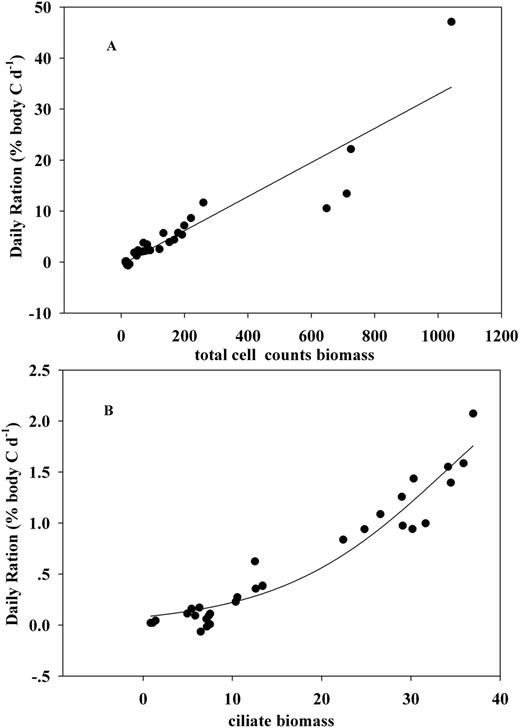
Regression curves of daily ration against cell counts biomass (A) and ciliate biomass (B).

Feeding selectivity

We focus on five experiments (E4, E5, E6, E7, E9) in which food diversity and concentrations of specific prey were high enough to examine feeding preference. Each experiment corresponded to a specific phase during the upwelling season.

Based on filtration rate (F)

Tukey–Kramer tests showed that the two larger Chl-a fractions, >20 µm and 5–20 µm, had similar filtration rates (94.2 and 106.6 mL euphausiid⁻¹ h⁻¹, Table VI, P = 0.6465), and both were significantly higher than the <5 µm fraction (35.9 mL euphausiid⁻¹ h⁻¹, P < 0.0002 and P < 0.0001, respectively). From June to August, F varied greatly on each of the cell count categories (Table VII) with overall higher values on the >30 µm single diatoms and chain diatoms; higher F were observed on the larger cells of both ciliates and dinoflagellates (>40 and >30 µm, respectively) except for E5.

Table VI:

Comparisons of filtration rate (F, mL euphausiid⁻¹ h⁻¹) between each pair of the Chl-a size fractions based on data from E3 to E9

Chl-a	Mean F	Lower 95% CI	Upper 95% CI	<5 µm	5–20 µm	>20 µm
<5 μm	35.9	16.3	55.5	–	–	–
5–20 µm	94.2	74.6	113.8	<0.0002a	–	–
>20 µm	106.6	87	126.2	<0.0001a	0.6465	–

^aTukey–Kramer HSD significance test (P = 0.01); CI, confidential interval.

Table VII:

Comparisons of average filtration rate (F ± SD, mL euphausiid⁻¹ h⁻¹) on different sizes of prey categories based on microscopic cell counts

Expt.#	Date	Single diatom (>30 μm)	Chain diatom	Small dino. (<30 μm)	Large dino. (>30 μm)	Small ciliate (<40 μm)	Large ciliate (>40 μm)	Flagellates (5-20 μm)
E4	8 June	199 ± 46	158 ± 79	101 ± 20	138 ± 59	192 ± 25	262 ± 51	83 ± 175
E5	19 June	237 ± 78	240 ± 81	182 ± 19	177 ± 27	208 ± 65	186 ± 18	178 ± 147
E6	27 June	165 ± 102	153 ± 69	51 ± 210	91 ± 38	66 ± 50	91 ± 62	81 ± 42
E7	21 July	121 ± 7	137 ± 80	na	98 ± 19	47 ± 81	94 ± 9	76 ± 18
E9	21 August	93 ± 23	85 ± 42	61 ± 7	88 ± 99	63 ± 68	53 ± 62	54 ± 64

Based on electivity indices (E_i)

During E4, which occurred early in the upwelling season (but with downwelling prevailing at the time of the cruise), ciliates dominated the total cell count biomass (∼70%) and were more preferred in terms of relatively higher E_i on Mesodinium rubrum (0.28) and small naked ciliates (0.15) (Fig. 6). Small flagellates (5–20 µm), silicoflagellates and the diatom Asterionellopsis glacialis were weakly selected (E_i = ∼0.1). Prey abundance and type were the predominant factors affecting selectivity for this period.

Fig. 6.

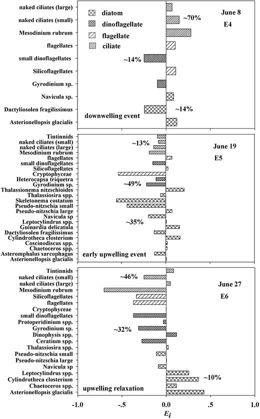
Selective feeding determined by electivity index (E_i, values from −1 to 1) in E4 to E6. Negative values of E_i indicate avoidance and positive values indicate preference. The three percentages, labeled from top to bottom on each of the plots, are proportions of ciliate, dinoflagellate and diatom carbon biomass, respectively.

In E5, during an early upwelling event in June (Fig. 6), the proportion of diatom carbon biomass was elevated significantly, up to ∼35%, as were dinoflagellates (∼49% higher). Some dominant diatoms (Table VIII) were preferred albeit in a weak way, e.g. large Pseudo-nitzschia with E_i = 0.07, Leptocylindrus spp. and Asterionellopsis glacialis each with E_i = 0.01; less abundant diatoms Cylindrotheca closterium, Guinardia delicatula and Thalassionema nitzschioides were positively selected at a higher preference level (0.16–0.20). In E5, E. pacifica mostly avoided the less abundant prey, e.g. diatoms Skeletonema costatum (−0.56), small Pseudo-nitzschia (−0.44), the dinoflagellate Gyrodinium sp. and ciliates (−0.08 to −0.19), but also some of the abundant items, e.g. Thalassiosira spp. (−0.06), Heterocapsa triquetra (−0.11), small dinoflagellates (−0.16) and Cryptophyceae (−0.54).

Table VIII:

Main species which occurred in five experiments (E4 to E7, and E9) were used for selectivity analysis

Expt. #	E4	E5	E6	E7	E9
Dominant prey	Carbon biomass (µg C L−1)
Asterionellopsis spp.	–	5.1 (0.6)	0.3 (0.1)	–	–
Cerataulina pelagic	–	–	–	2.3 (0.4)	14.3 (1.9)
Chaetoceros spp.	–	0.5 (0.1)	0.2 (0.04)	36.9 (5.0)	457.7 (46.2)
Coscinodiscus spp.	–	8.1 (0.8)	–	–	–
Cylindrotheca closterium	–	–	0.1 (0.02)	–	–
Dactyliosolen fragilissimus	–	0.1 (0.02)	–	2.2 (0.2)	16.9 (3.1)
Eucampia zodiacus	–	–	–	3.2 (0.6)	17.0 (2.4)
Guinardia delicatula	–	1.1 (0.1)	–	6.2 (1.3)	–
Lauderia annulata				61.2 (6.5)	8.2 (0.8)
Leptocylindrus spp.	–	19.2 (4.6)	1.8 (0.2)	17.0 (2.1)	36.9 (6.8)
Navicula spp.		–	0.2 (0.02)	–	–
Pseudo-nitzschia spp.	–	23.4 (1.8)	3.0 (0.4)	3.2 (0.5)	1.7 (0.1)
Skeletonema spp.	–	–	–	1.5 (0.4)	37.1 (3.4)
Thalassionema nitzschioides	–	–	–	–	–
Thalassiosira spp.	–	9.0 (0.4)	1.5 (0.3)	7.3 (0.3)	43.8 (6.4)
Ceratium spp.	1.0 (0.3)	0.4 (0.1)	1.4 (0.2)	1.4 (0.2)	–
Dinophysis spp.	–	0.3 (0.1)	6.5 (0.3)	0.2 (0.1)	–
Gyrodinium sp.	1.3 (0.1)	0.9 (0.1)	0.8 (0.1)	0.5 (0.1)	2.5 (0.4)
Protoperidinium spp.	0.3 (0.1)	1.2 (0.2)	7.3 (0.7)	2.9 (0.3)	3.2 (0.5)
Small dinoflagellates	1.5 (0.1)	8.4 (2.2)	2.5 (0.6)	–	11.0 (1.4)
Heterocapsa triquetra	–	11.9 (0.9)	–	–	–
Cryptophyceae	1.3 (0.1)	2.5 (0.3)	1.1 (0.2)	1.1 (0.2)	1.4 (0.2)
Euglenophyceae	–	0.2 (0.04)	0.2 (0.02)	–	–
Silicoflagellates	0.4 (0.04)	0.4 (0.02)	–	0.2 (0.01)	0.2 (0.04)
flagellates (5–20 µm)	0.8 (0.1)	1.1 (0.2)	6.1 (0.8)	1.5 (0.3)	2.5 (0.3)
Mesodinium rubrum	4.0 (0.3)	–	0.4 (0.04)	2.6 (0.2)	0.4 (0.2)
Naked ciliates (<40 µm)	10.7 (0.7)	7.1 (0.6)	5.3 (0.42)	2.3 (0.2)	1.2 (0.2)
Naked ciliates (>40 µm)	19.4 (1.4)	5.9 (0.5)	11.2 (0.7)	5.6 (0.7)	4.9 (0.4)
Tintinnids	–	10.2 (0.5)	14.9 (0.9)	–	2.3 (0.3)

Bold fonts are the carbon biomass (standard deviation in brackets) of those especially dominant species. “–” indicates species absent or inconsistent appearing in individual experiment.

E6 was done during an upwelling relaxation event. Diatom biomass declined to ∼10% of the total, while ciliate and dinoflagellate biomass increased (∼46 and ∼32%, respectively) (Fig. 6). Euphausia pacifica preferred some less abundant diatoms (Table VIII), such as Asterionellopsis glacialis (0.43), Cylindrotheca closterium (0.36) and Leptocylindrus spp. (0.25). Selection was weaker, on the abundant dinoflagellate Dinophysis spp. (0.12), large naked ciliates (0.05) and tintinnids (0.08).

E7 was done during a strong upwelling event (Fig. 7). Diatoms dominated the prey community (∼87%). Euphausia pacifica showed a preference for a few dominant diatoms, such as Eucampia zodiacus (0.36), large Pseudo-nitzschia (0.24), but lesser preference for the more abundant Guinardia delicatula (0.11), and Chaetoceros spp. (0.07). Again higher preference was observed on the less dominant species Asterionellopsis glacialis (0.43) and Skeletonema costatum (0.29). They avoided several dominant diatoms like Lauderia annulata (−0.26) and Leptocylindrus spp. (−0.14), but mostly avoided less abundant prey, e.g. Cerataulina pelagica (−0.5), small Pseudo-nitzschia (−0.42), Dactyliosolin fragilisimus (−0.23), Gyrodinium spp. (−0.27) and ciliates (−0.43). The observed within-diatom selection appeared to be associated with species abundance and shape.

Fig. 7.

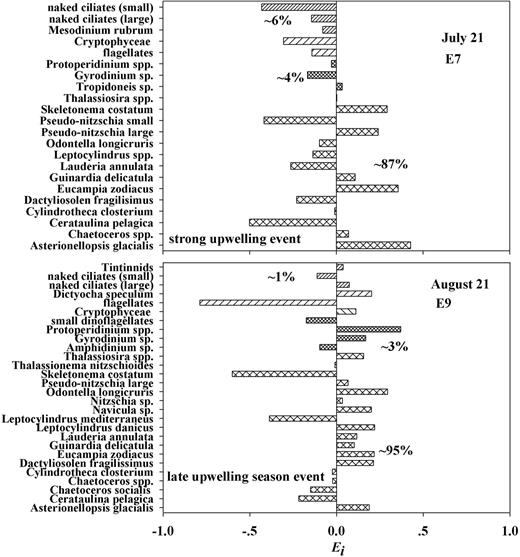
Selective feeding was determined by electivity index in E7 and E9. Definitions are all the same to Fig. 6.

For E9 during a late-season upwelling event (Fig. 7), diatoms were overwhelmingly dominant (∼95% carbon contribution). Euphausia pacifica either preferred (0.03 to 0.29) or avoided (−0.6 to −0.01) diatoms but both irrespective of diatom abundance. Although ciliates and dinoflagellates were trivial numerically compared with diatoms, their larger taxa, such as large naked ciliates (0.07), tintinnids (0.04), Dinophysis spp. (0.17) and Protoperidinium spp. (0.37), were selected at different levels.

DISCUSSION

Filtration rate

There is little published information showing how E. pacifica filtration rate responds to a range of food concentrations. Our results mostly are similar, to, but somewhat higher than previous studies. Ohman (Ohman, 1984) reported rates ranging from 25 to 150 mL euphausiid⁻¹ h⁻¹ when feeding on a diatom species, similar to our rates when feeding on “natural” diatoms; there are reports of rates of 30–75 mL euphausiid⁻¹ h⁻¹ on marine snow and TEP (Dilling et al., 1998; Passow and Alldredge, 1999), similar to our rates of 35 mL euphausiid⁻¹ h⁻¹ on the <5 µm size fraction of Chl-a. This indicates that both marine snow and TEP serve as alternative food sources for krill that are found offshore of the California Current and the Transition Zone, which may be one of the reasons why they can survive and even prosper in relatively oligotrophic waters of the North Pacific. The filtration rates on ciliates which we measured (an average of 137 and maximum of 262 mL euphausiid⁻¹ h⁻¹) were lower than the range (140–840 mL euphausiid⁻¹ h⁻¹) for ciliates in waters off Japan (Nakagawa et al., 2004).

We observed both the lowest and the higher filtration rates at the lower range of food concentrations in terms of both Chl-a and carbon. This demonstrates that bulk measures of food concentration do not predict filtration rate. The most likely explanation for the unexpectedly high filtration rates at low Chl-a for E4 and E5 is that the krill were feeding on motile prey like ciliates besides diatoms. Since ciliates usually are far less abundant than diatoms, this suggests different modes while capturing motile versus non-motile prey. Similarly, Euphausia superba was found to feed raptorially on motile taxa (Atkinson and Synder, 1997) but to display classic filter feeding on diatoms.

Percent swept clear averaged 16.0% in three low Chl-a experiments (E2, E3 and E6), but 67.7% in the other two low Chl-a experiments (E4 and E5). Given that our target was ∼30% removal, we note that in the first three experiments, the percent swept cleared was calculated soon after the end of each experiment so that we could determine whether we were close to our target of a maximum of 30–40% removal suggested by Gifford (Gifford, 1993). Since we were close to our target, we felt confident that having five adult krill grazing for 8 h in 4 L containers was the appropriate balance of number of grazers, length of experiment and size of container. Thus, we were quite surprised to find values approaching 70%. We did use “average” food concentration for our calculations of filtration rate (Marin et al., 1986) rather than “initial” or “final” concentration which reduces the bias in the filtration calculations. However, we note that the calculation of “percent swept clear” is a subjective exercise because in reality it should be calculated based on numbers or mass of each taxa or species that was consumed, not on bulk measures of biomass. Given that one of the goals of this study was to estimate filtration and ingestion rates of krill on specific taxa and species, not total microplankton biomass, the calculations of electivity are perhaps of greater interest instead of bulk filtration rates.

Ingestion rate

Ingestion rates of 4.8–16.1 µg C euphausiid⁻¹ h⁻¹ over a concentration range of 70–200 µg C L⁻¹ in our study are comparable with rates on a cultured diatom (up to 14 µg C euphausiid⁻¹ h⁻¹) (Ohman, 1984), marine snow (9–15 µg C euphausiid⁻¹ h⁻¹) (Dilling et al., 1998) and on transparent exopolymer particles (8–18 µg C euphausiid⁻¹ h⁻¹) (Passow and Alldredge, 1999). Ingestion rates of 0.02–2.98 µg C euphausiid⁻¹h⁻¹ on ciliates in our experiments are also similar to the range of 0.06–1.95 µg C euphausiid⁻¹h⁻¹ reported from coastal waters off Japan (Nakagawa et al., 2004).

Ingestion rate as a function of food concentrations fits linear (type I), type II and III models depending on prey variables (total cell count biomass and Chl-a size fractions), all of which shared a common characteristic in that neither model suggested that satiated feeding was occurring. Similar results were reported for E. superba (Ross et al., 1998) and for Thysanoessa raschii (McClatchie, 1988). In both studies, ingestion rates continued to increase linearly at Chl-a concentrations >10–12 μg L⁻¹. Concerning our type II models on total Chl-a and Chl-a >20 μm fraction, Parsons et al. (op.cit) also obtained a type II response for E. pacifica feeding on the diatom Chaetoceros. Ohman (Ohman, 1984) reported a type III response on the diatom Thalassiosira angstii, as did Agersted et al. (Agersted et al., 2011) for T. raschii, feeding on cultured Thalassiosira weissflogii. Ingestion rate against ciliates fits a type III sigmoidal model in our experiments, the same as for the response of Nyctiphanes australis to the small copepod Acartia spp. (Pilditch and McClatchie, 1994). The type III response was noted as an adaption to changeable food conditions which in turn may regulate in situ prey density (Holling, 1959); therefore, its ecological meaning lies in enhancing ecosystem stability. Mechanisms causing different functional responses, e.g. encounter feeding have been discussed by Mauchline (Mauchline, 1980). The importance of prey characteristics, e.g. mobility and biochemistry, has been highlighted (Hassell, 1978). Though there is no conclusive result, this study at least demonstrates that in the upwelling zone off Oregon, changes from a type II to a type III feeding response seem to relate to changes in prey types from algal autotrophs to more motile heterotrophs.

Daily ration (DR)

The maximum daily ration (DR) of 23% on only phytoplankton at the highest food biomass of ∼700 µg C L⁻¹ was comparable to the highest DR of 20% reported by Ross when the prey, Thalassiosira weissflogii, exceeded 350 µg C L⁻¹ (Ross, 1982). Other published records include a maximum DR of 15% on the diatom Chaetoceros (Parsons et al., 1967), 8.8% on the diatom Thalassiosira angstii (Ohman, 1984), 5–10% on marine snow (Dilling et al., 1998) and 0.04–19.73% on natural phytoplankton (Nakagawa et al., 2004), all of which fall within the range of our observations (Fig. 8).

Fig. 8.

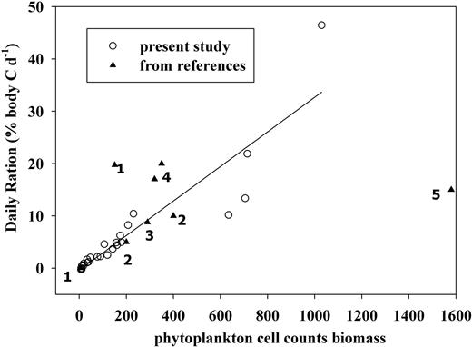
Linear regression between daily ration (empty circles) and phytoplankton carbon biomass (R² = 0.84, P < 0.0001). Filled triangles (numbered as 1–5) represent values from previous studies. (1, Nakagawa et al., 2004; 2, Dilling et al., 1998; 3, Ohman, 1984; 4, Ross, 1982; 5, Parsons et al., 1967).

At 12 and 8°C, 2–4% of the daily ration of E. pacifica was sufficient to maintain regular growth, respiration and molting (Ross, 1982). Lasker (Lasker, 1966) suggested ∼5% for the overall maintenance. In our study, high daily rations were seen only during three experiments during the upwelling season in late June (DR = 7.6%), late July (5.6%) and late August (23.3%), suggesting that sufficient food to meet or exceed daily requirements were found only during diatom blooms. During the early phase of the upwelling season and non-bloom period, daily rations (2.5 and 2.4%) were probably just close to the lower limit. Thus, before the initiation of the upwelling season, E. pacifica likely never reached the carbon requirement from their food ingestion to grow at high rates except possibly in February during years when a late-winter bloom was observed (Feinberg et al., 2010). This may explain why maximum egg production rates of E. pacifica in our study region are usually observed only during the summer upwelling season (Feinberg et al., 2007). Moreover, availability of food resources explains why growth reaches a maximum in summer, is slow in spring, but negative in winter (Shaw et al., 2010).

Particle size as a factor of feeding selectivity

Apart from particles <5 µm in diameter which were fed upon at lower rates, we found that prey size alone did not seem to determine E. pacifica feeding selectivity when all available particles (mostly < 200 μm) were within the edible size range. This is similar to what Decima (Decima, 2011) found in that there was no consistent pattern in prey size or type consumed by E. pacifica in experiments carried out in the southern California Current ; E. pacifica might filter feed on food particles <50 μm, and feed raptorially on particles above 50 μm (Jorgensen, 1966). The upper limit is not easily defined and likely related to the alteration of feeding styles which would ensure E. pacifica has the ability to eat a wide size spectrum of prey types with different degrees of mobility.

However, larger particles did impact feeding effort more obviously. Higher filtration rates were measured on larger phytoplankton taxa and the >20 μm Chl-a fraction; larger dinoflagellates and ciliates were predominantly preferred to their smaller types; smaller flagellates were positively selected but only when larger phytoplankton and ciliates were lacking. Compared with other krill, Nyctiphanes australis similarly gained much of their carbon from larger prey (Pilditch and McClatchie, 1994); Euphausia superba might somehow compact small taxa into a large bolus in order to ingest them efficiently (Haywood and Burns, 2003).

Meanwhile, other factors could complicate the effect of “size” on selectivity, e.g. prey morphology. We observed long-chain diatoms (such as Chaetoceros spp.) were sometimes avoided when they were at especially high density. The fine mesh of the E. pacifica feeding basket could be easily clogged by long silicious setae of Chaetoceros spp. (Parsons et al., 1967; Suh and Choi, 1998). Long-chain species probably need more handling time too; thus we suggest that E. pacifica would rather choose less abundant single cells or short-chain diatoms. Prey availability is undoubtedly considered by E. pacifica: ciliates were preferred at high biomass, and diatoms were consumed almost exclusively during summer blooms. Large dinoflagellates were seldom eaten preferably perhaps due to their low abundance. More physiological concepts, such as optimal efficiency, opportunistic feeding, nutritional necessity, inherent adaption, etc. perhaps account for the selectivity but are difficult to detect and quantify.

Contribution of ciliates to the diet of E. pacifica

The greatest relative contribution of ciliates to the diet of E. pacifica came in the early and weak part of the upwelling season and before diatoms dominated the microplankton in summer. Ciliates contributed 1.3% of daily ingested carbon during post-bloom periods (E6 and E8), 1.4% during pre-bloom (early June) but only 0.2% during summer phytoplankton blooms; therefore, we suggest that ciliates alone may not be sufficient to fulfill the daily carbon needs of E. pacifica in waters of the northern California Current. In contrast, in waters off Japan, naked ciliates alone could meet much of E. pacifica per day energy requirement (Nakagawa et al., 2004).

Trophic interactions biasing feeding rates

It is well established that micro-grazers (ciliates and heterotrophic dinoflagellates) within the incubation bottles cause different feeding effects on their likely prey (Calbet and Landry, 2004) which in turn could bias the estimate of feeding rate of E. pacifica on phytoplankton prey. However, the complexity of the effects of “trophic cascades” makes it difficult to estimate grazing rates accurately because different size categories usually act at more than one trophic role in the ocean food web. Thus given that microzooplankton (ciliates and heterotrophic dinoflagellates) might have been feeding on the same foods as E. pacifica in our experiments, it is possible that our filtration and ingestion rates are biased. On the one hand, ciliates were feeding at unknown rates on small cells in the control bottles and on the other hand, E. pacifica fed on ciliates when they were abundant; thus the ciliates may not have had a large impact in the grazing bottles because their biomass was kept low, an average reduction of 65% over all experiments (range of 33–87%). Also, noting that E. pacifica clearly preferred larger cells (>20 µm) and that ciliates seem to prefer nano- and pico-plankton that are <5 µm, we hypothesize that ciliate grazing on small cells has minimal impact on calculations of krill filtration rates because krill fed on these small cells at very low rates (as shown in Table VI). Grazing by heterotrophic dinoflagellates remain a problem since we really do not know if the taxa we classified as “heterotrophic dinoflagellaes” were accurate due to the use of Lugol's as a preservative. Regardless, two methods have been suggested for correcting potential biases. One method is to combine incubation experiments with mass-balance ecosystem models to correct for trophic cascade effects, an idea proposed by Klaas et al. (Klaas et al., 2008). Another method is to conduct both bottle incubation and dilution experiments at the same time in order to directly measure and correct for the possible underestimate caused by microzooplankton grazing (Nejstgaard et al., 2001). Each of these methods is well beyond the scope of our work but seem reasonable to be taken in future studies by a larger team of researchers.

CONCLUSIONS

The ability of E. pacifica to occupy a broad range of habitats over the North Pacific must be linked to its ability to adapt to changeable food sources and to feed on a large variety of available prey, ranging from smaller flagellates to larger single or long-chain phytoplankton as well as microzooplankton. Within the unique coastal upwelling system in the northern California Current, we found E. pacifica fed omnivorously on particles from autotrophic prey (mostly diatoms and flagellates) to heterotrophic prey (ciliates and heterotrophic dinoflagellates); feeding intensity varied with upwelling status and the resultant food availability; the highest feeding rates and greatest daily rations were obtained by E. pacifica during the upwelling season-diatom blooms; selective feeding was found between and within the main functional groups (diatoms, flagellates, ciliates) and again was upwelling and food availability dependent; prey type, abundance, shape and size were the likely factors causing selectivity.

FUNDING

This work was supported by the NOAA/MERHAB 2007 program project (NA07NOS4780195) (MOCHA); and the NOAA/CAMEO program (NA09NMF4720182). The research was part of the PhD Dissertation of Xiuning Du carried out with the support of the China Scholarship Council.

Acknowledgements

We thank all the people in Peterson lab, the Captains on the R/V Elakha and volunteers in HMSC for collecting samples and giving me a hand for setting up experiments. Tracy Shaw and Jay Peterson provided constructive comments on this manuscript.

Author notes

Corresponding editor: Marja Koski