Effects of chiral three-nucleon forces on ⁴He-nucleus scattering in a wide range of incident energies

Abstract

An important current subject is to clarify the properties of chiral three-nucleon forces (3NFs) not only in nuclear matter but also in scattering between finite-size nuclei. Particularly for elastic scattering, this study has just started and the properties are not understood for a wide range of incident energies (⁠|$E_{\rm in}$|⁠). We investigate basic properties of chiral 3NFs in nuclear matter with positive energies by using the Brueckner–Hartree–Fock method with chiral two-nucleon forces at N|$^{3}$|LO and 3NFs at NNLO, and analyze the effects of chiral 3NFs on |$^{4}$|He elastic scattering from targets |$^{208}$|Pb, |$^{58}$|Ni, and |$^{40}$|Ca over a wide range of |$30 \underset{\raise0.3em\hbox{$\smash{\scriptscriptstyle\thicksim}$}}{<} E_{\rm in}/A_{\rm P} \underset{\raise0.3em\hbox{$\smash{\scriptscriptstyle\thicksim}$}}{<} 200$| MeV by using the |$g$|-matrix folding model, where |$A_{\rm P}$| is the mass number of the projectile. In symmetric nuclear matter with positive energies, chiral 3NFs make the single-particle potential less attractive and more absorptive. The effects mainly come from the Fujita–Miyazawa 2|$\pi$|-exchange 3NF and become slightly larger as |$E_{\rm in}$| increases. These effects persist in the optical potentials of |$^{4}$|He scattering. As for the differential cross sections of |$^{4}$|He scattering, chiral-3NF effects are large for |$E_{\rm in}/A_{\rm P} \underset{\raise0.3em\hbox{$\smash{\scriptscriptstyle\thicksim}$}}{>} 60$| MeV and improve the agreement of the theoretical results with the measured ones. Particularly for |$E_{\rm in}/A_{\rm P} \underset{\raise0.3em\hbox{$\smash{\scriptscriptstyle\thicksim}$}}{>} 100$| MeV, the folding model reproduces measured differential cross sections pretty well. Cutoff (⁠|$\Lambda$|⁠) dependence is investigated for both nuclear matter and |$^{4}$|He scattering by considering two cases of |$\Lambda=450$| and |$550$| MeV. The uncertainty coming from the dependence is smaller than chiral-3NF effects even at |$E_{\rm in}/A_{\rm P}=175$| MeV.

1. Introduction

How do three-nucleon forces (3NFs) work in nuclear many-body systems? This is an important subject to be answered in nuclear physics. Even if 3NFs do not exist on a fundamental level, they come out in effective theories with a finite momentum cutoff |$\Lambda$| by renormalizing the degrees of freedom present above |$\Lambda$|⁠. The representative example is the 2|$\pi$|-exchange process with intermediate nucleon excited states, typically the |$\Delta(1232)$| isobar. It is now called the Fujita–Miyazawa 3NF [1,2]. As a phenomenological approach, attractive 3NFs were introduced to reproduce the binding energies for light nuclei [3], whereas repulsive 3NFs were used to explain the empirical saturation properties in symmetric nuclear matter [4].

Essential progress on this subject was made by chiral effective field theory (EFT); [5,6] based on chiral perturbation theory. The theory provides a low-momentum expansion of two-nucleon force (2NF), 3NF, and many-nucleon forces, and makes it possible to define the forces systematically. Figure 1 shows chiral 3NFs in the next-to-next-to-leading order (NNLO). Figure 1(a) corresponds to the Fujita–Miyazawa 2|$\pi$|-exchange 3NF [1,2], and (b) and (c) represent the 1|$\pi$|-exchange and contact 3NFs, respectively. The filled-square vertex has a strength |$c_D$| in (b) and |$c_E$| in (c). Quantitative roles of chiral 3NFs have been extensively investigated, particularly for light nuclei and nuclear matter [7]; more precisely, see Ref. [8] for light nuclei, Refs. [9,10] for ab initio nuclear-structure calculations in lighter nuclei, and Refs. [11–17] for nuclear matter. In addition, effects of chiral four-nucleon forces were found to be small in nuclear matter [18,19]. The chiral |$g$| matrix, calculated from chiral 2NF+3NF with the Brueckner–Hartree–Fock (BHF) method, yields a reasonable nuclear matter saturation curve for symmetric nuclear matter, when the parameters, |$c_{D}$| and |$c_{E}$|⁠, of NNLO 3NFs are tuned [14].

Fig. 1.

3NFs in NNLO. Diagram (a) corresponds to the Fujita–Miyazawa 2|$\pi$|-exchange 3NF [1,2], and diagrams (b) and (c) correspond to 1|$\pi$|-exchange and contact 3NFs. The solid and dashed lines denote nucleon and pion propagations, respectively, and filled circles and squares stand for vertices. The strength of the filled-square vertex is often called |$c_{D}$| in diagram (b) and |$c_{E}$| in diagram (c).

Nuclear scattering is another place to investigate 3NF effects. The theoretical description of |$N$|+|$d$| scattering has been naturally associated with the necessity of 3NFs [8,20], when the theory starts with sophisticated 2NFs determined from experiments. Microscopic evaluation of nuclear optical potentials for nucleon–nucleus (NA) and nucleus–nucleus (AA) elastic scattering has a long history. The |$g$|-matrix folding model [21–28] is a standard method for deriving the optical potentials of NA and AA elastic scattering microscopically. In fact, the potentials have been used to analyze various kinds of nuclear reactions in many papers. In the model, the optical potentials were obtained by folding the |$g$| matrix [21–28] with the projectile (P) density |$\rho_{\rm P}$| and the target (T) one |$\rho_{\rm T}$|⁠. This description has been quite successful in explaining many elastic scatterings. At first, the effects of 3NFs were phenomenologically investigated in Ref. [26] for NA elastic scattering and in Refs. [25,29] for NA and AA elastic scattering. The 3NFs reduce differential cross section and improve the agreement with measured vector analyzing powers. However, the role of 3NFs has not been clarified quantitatively, because the folding potential is adjusted to measured cross sections.

In Refs. [30,31], as a first attempt, we presented a qualitative discussion for chiral-3NF effects on elastic scattering by using the hybrid method in which the existing local version of the Melbourne |$g$| matrix [24] was modified on the basis of the chiral |$g$| matrix constructed from chiral 2NFs and 3NFs. The work showed that chiral-3NF effects are small for NA elastic scattering, but important for AA elastic scattering. Recently, we directly parameterized the chiral |$g$| matrix as a local potential based on chiral 2NF+3NF, as briefly reported in Ref. [28]. In this paper, we present a full understanding of chiral-3NF effects on |${^4}$|He elastic scattering over a wide range of |$30 \underset{\raise0.3em\hbox{$\smash{\scriptscriptstyle\thicksim}$}}{<} E_{\rm in}/A_{\rm P} \underset{\raise0.3em\hbox{$\smash{\scriptscriptstyle\thicksim}$}}{<} 200$| MeV (where |$E_{\rm in}$| is the incident energy in the laboratory system and |$A_{\rm P}$| is the mass number of the projectile) by using the local version of the chiral |$g$| matrix.

The |$g$| matrices calculated so far are provided by a local potential with Yukawa or Gaussian form, since this procedure makes the folding calculation much easier.

Investigation of chiral-3NF effects on NA and AA elastic scattering has just started with lower incident energies per nucleon such as |$E_{\rm in}/A_{\rm P} \approx 70$| MeV by using the |$g$|-matrix folding model [28,30,31], since chiral EFT is more reliable for lower incident energies. As mentioned above, the folding potentials were recently calculated from the local version of the chiral |$g$| matrix in Ref. [28]. The chiral |$g$|-matrix folding model accounts for experimental data reasonably well on NA scattering at |$E_{\rm in}=65$| MeV and |$^{4}$|He+|$^{58}$|Ni scattering at |$E_{\rm in}/A_{\rm P}=72$| MeV. This model also showed that chiral-3NF effects are small for NA elastic scattering, but sizable for |$^{4}$|He elastic scattering.

In our previous studies for |$^4$|He elastic scattering, we used the Melbourne |$g$| matrix in Ref. [32] and the chiral |$g$| matrices based on chiral 2NF and chiral 2NF+3NF in Ref. [28]. After Ref. [28] was published, we found some numerical errors in our nuclear-matter calculations including chiral 3NFs; see Ref. [33] for the details. In the present work, we adopt the corrected version of the chiral |$g$| matrix; see Appendix A for the matrix. See also the further discussion in Sect. 2.2.

In this paper, we first investigate basic properties of chiral 3NFs in symmetric nuclear matter for positive energies up to 200 MeV by using the BHF method with chiral 2NFs of N|$^{3}$|LO and chiral 3NFs of NNLO. We show that chiral-3NF effects provide density-dependent repulsive and absorptive corrections to the single-particle potential, and that the effects become slightly larger as the energy increases. We also point out that the corrections mainly come from the Fujita–Miyazawa 2|$\pi$|-exchange 3NF of Figure 1(a).

Second, we analyze chiral-3NF effects on |$^{4}$|He scattering from various targets in a wide range of incident energies by using the chiral |$g$|-matrix folding model. In order to make our discussion clear, we take |$^{4}$|He scattering as AA scattering, since the |$g$|-matrix folding model is confirmed to work well for |$^{4}$|He scattering in virtue of negligibly small projectile-breakup effects [32,34]; see Sect. 2.4 for further discussion. In addition, as targets we take heavier nuclei, |$^{208}$|Pb, |$^{58}$|Ni, and |$^{40}$|Ca, since the |$g$| matrix is evaluated in nuclear matter and is considered to be more suitable for heavier targets. For the targets, experimental data are available in a wide range of |$30 \underset{\raise0.3em\hbox{$\smash{\scriptscriptstyle\thicksim}$}}{<} E_{\rm in}/A_{\rm P} \underset{\raise0.3em\hbox{$\smash{\scriptscriptstyle\thicksim}$}}{<} 200$| MeV.

In the present paper, we mostly consider the case of the cutoff scale |$\Lambda=550$| MeV. As the third subject, |$\Lambda$| dependence is investigated for nuclear matter with positive energies and |$^{4}$|He elastic scattering by taking two other cases of |$\Lambda=450$| and |$550$| MeV.

Finally, we provide the local version of the chiral |$g$| matrix including chiral-3NF effects with a three-range Gaussian form for the case of |$E_{\rm in}/A_{\rm P}=75$| MeV. This may strongly encourage the application of the chiral |$g$| matrix for studying various kinds of nuclear reactions. This local version of the chiral |$g$| matrix is referred to as the “Kyushu chiral |$g$| matrix” in this paper.

In Sect. 2, we present the theoretical framework composed of the BHF method and the folding model, and show some basic results of BHF calculations for chiral 2NF+3NF. In Sect. 3, the results of the chiral |$g$|-matrix folding model are shown for |$^{4}$|He elastic scattering. Section 4 is devoted to a summary.

2. Theoretical framework and basic results

2.1. BHF equation for 2NF+3NF

We first recapitulate the BHF method for 2NF+3NF, following Ref. [13]. Because it is not easy to treat a 3NF |$V_{123}$| even in nuclear matter, we introduce an effective 2NF |$V_{12}^{\rm eff}$| by applying the mean-field approximation, or the normal ordering prescription, to the 3NF:

\begin{eqnarray} \frac{1}{2} \sum_{{\boldsymbol{k}}_1 {\boldsymbol{k}}_2} \langle {\boldsymbol{k}}_1 {\boldsymbol{k}}_2 | V_{12} |{\boldsymbol{k}}_1 {\boldsymbol{k}}_2\rangle_{\cal A} +\frac{1}{3}!\sum_{{\boldsymbol{k}}_1 {\boldsymbol{k}}_2 {\boldsymbol{k}}_3} \langle {\boldsymbol{k}}_1 {\boldsymbol{k}}_2 {\boldsymbol{k}}_3| V_{123} |{\boldsymbol{k}}_1 {\boldsymbol{k}}_2 {\boldsymbol{k}}_3\rangle_{\cal A} =\frac{1}{2} \sum_{{\boldsymbol{k}}_1 {\boldsymbol{k}}_2} \langle {\boldsymbol{k}}_1 {\boldsymbol{k}}_2 | V_{12}^{\rm eff} |{\boldsymbol{k}}_1 {\boldsymbol{k}}_2\rangle_{\cal A} , \label{pot-energy} \end{eqnarray}

(1)

where |${\cal A}$| represents antisymmetrization and |${\boldsymbol{k}}_i$| corresponds to the quantum numbers of the |$i$|th nucleon. Equation (1) leads to

\begin{eqnarray} V_{12}^{\rm eff}=V_{12}+ \frac{1}{3}V_{12(3)} , \label{eff-V12} \end{eqnarray}

(2)

where |$V_{12(3)}$| is defined by summing 3NF |$V_{123}$| over the third nucleon in the Fermi sea:

\begin{equation} \langle {\boldsymbol{k}}_1' {\boldsymbol{k}}_2' | V_{12(3)} |{\boldsymbol{k}}_1 {\boldsymbol{k}}_2\rangle_{\cal A} = \sum_{{\boldsymbol{k}}_3} \langle {\boldsymbol{k}}_1' {\boldsymbol{k}}_2' {\boldsymbol{k}}_3 | V_{123} |{\boldsymbol{k}}_1 {\boldsymbol{k}}_2 {\boldsymbol{k}}_3 \rangle_{\cal A} , \end{equation}

(3)

assuming the center-of-mass (c.m.) frame: |${\boldsymbol{k}}_1'+{\boldsymbol{k}}_2'={\boldsymbol{k}}_1+{\boldsymbol{k}}_2$|⁠. Note the factor |$1/3$| in Eq. (2). The |$g$| matrix |$g_{12}$| is a solution to the BHF equation

\begin{equation} g_{12}=V_{12}^{\rm eff}+V_{12}^{\rm eff} G_0 g_{12} , \label{g-eq} \end{equation}

(4)

where |$G_0$| is the nucleon propagator with the Pauli exclusion operator in the numerator and with the single-particle energy

\begin{eqnarray} e_{{\boldsymbol{k}}}=\langle {\boldsymbol{k}} |T|{\boldsymbol{k}}\rangle + {\rm Re}[{\cal U}({\boldsymbol{k}})] \end{eqnarray}

(5)

of the nucleon having a momentum |${\boldsymbol{k}}$| in the denominator. Here, |$T$| is the standard kinetic-energy operator of the nucleon, and the single-particle potential |${\cal U}({\boldsymbol{k}})$| is defined by [13]

\begin{eqnarray} {\cal U}({\boldsymbol{k}}) = \sum_{|{\boldsymbol{k}}'|\le k_{\rm F}} \langle {\boldsymbol{k}} {\boldsymbol{k}}' | \tilde{g}_{12} |{\boldsymbol{k}} {\boldsymbol{k}}' \rangle_{\cal A} , \label{single-particle-pot-0} \end{eqnarray}

(6)

with the effective |$g$| matrix, the so-called |$\tilde{g}$| matrix, including additional rearrangement terms of the 3NF origin:

\begin{eqnarray} \tilde{g}_{12}=g_{12} +\frac{1}{6} V_{12(3)}(1+G_0 g_{12}) . \label{effective-g} \end{eqnarray}

(7)

Note that |${\boldsymbol{k}}$| is related to the incident energy |$E_{\rm in }$| as |$E_{\rm in }=(\hbar {\boldsymbol{k}})^2/(2m) + {\rm Re}[{\cal U}]$|⁠. The present formulation is consistent with the second-order perturbation of Ref. [35], because of the factor |$1/6$| in Eq. (7). For symmetric nuclear matter where the proton density |$\rho_{p}$| agrees with the neutron one |$\rho_{n}$|⁠, the Fermi momentum |$k_{\rm F}$| is related to the matter density |$\rho=\rho_{p}+\rho_{n}$| as |$k_{\rm F}^3= 3\pi^2 \rho/2$|⁠, so that the normal density |$\rho=\rho_0=0.17$| fm|$^{-3}$| is realized at |$k_{\rm F}=1.35$| fm|$^{-1}$|⁠.

2.2. Some basic results of BHF calculations

The |$\tilde{g}$| matrix is calculated from the chiral 2NF of N|$^{3}$|LO and the chiral 3NF of NNLO by using the BHF method. In BHF calculations, the form factor |$\exp\{-(q'/\Lambda)^6-(q/\Lambda)^6\}$| is introduced for both |$V_{12}$| and |$V_{12(3)}$|⁠. We mainly consider the case of |$\Lambda=550$| MeV, and take another case |$\Lambda= 450$| MeV when the |$\Lambda$| dependence of physical quantities is estimated. The low-energy constants relevant for 3NFs are |$(c_1,c_3,c_4)=(-0.81,-3.4,3.4)$| [36] in units of GeV|$^{-1}$|⁠.

As noted earlier, some errors were found in the nuclear-matter calculations with chiral 3NFs of Ref. [13], after Ref. [28] was published. Although the qualitative importance of chiral 3NFs for improving nuclear matter saturation properties does not change, the saturation curve is changed by the corrections. To restore reasonable nuclear saturation properties, which are basically important for further application in microscopic derivation of nuclear optical potentials, the remaining two parameters |$c_D$| and |$c_E$| are tuned [33]. In consideration of the uncertainty that the |$c_D$| and |$c_E$| terms yield almost identical contributions when |$c_D \simeq 4c_E$|⁠, |$c_D$| is determined as |$-2.5$| by setting |$c_E=0$| for |$\Lambda=450$| MeV, and then |$c_E$| is fixed as |$0.25$| for |$\Lambda=550$| MeV, keeping |$c_D=-2.5$|⁠. These values are somewhat different from those determined in few-body systems within continuous uncertainties. It has been recognized [10], however, that low-energy constants fixed solely in few-body systems are not adequate in heavier systems. In this article, we use the corrected version of the chiral |$g$| matrix.

It is known that chiral 3NFs make repulsive corrections to the binding energy of symmetric nuclear matter [13]. What happens for positive energy? Figure 2 shows the |$E_{\rm in}$| dependence of |${\cal U}$| for the case of |$k_{\rm F}=1.2$| fm|$^{-1}$| for the cutoff |$\Lambda = 550$| MeV. This density is realized in the peripheral region of a target nucleus and is therefore important for elastic scattering. The filled (open) circles denote the results of BHF calculations with (without) chiral 3NFs. One can see that chiral 3NFs make |${\cal U}$| less attractive and more absorptive. The 3NF corrections slightly increase as |$E_{\rm in}$| increases. Our results are consistent with the second-order perturbation calculation by Holt et al. [35].

Fig. 2.

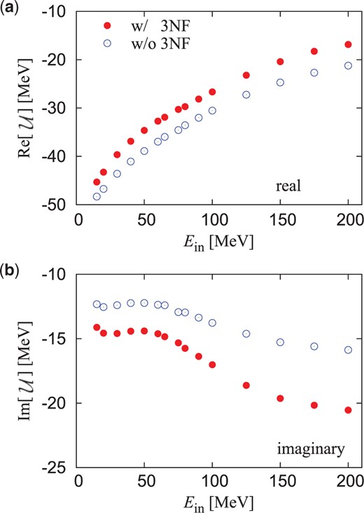
The |$E_{\rm in}$| dependence of |${\cal U}$| at |$k_{\rm F}=1.2$| fm|$^{-1}$| for the cutoff |$\Lambda = 550$| MeV. The filled (open) circles stand for the results of BHF calculations with (without) chiral 3NFs. Panels (a) and (b) correspond to the real and imaginary parts of |${\cal U}$|⁠.

Figure 3 shows |${\cal U}$| as a function of |$E_{\rm in}$| at |$k_{\rm F}=1.2$| fm|$^{-1}$|⁠, but two cases of |$\Lambda=450$| and |$550$| MeV are taken in the BHF calculations to see the uncertainty coming from |$\Lambda$| dependence on |${\cal U}$|⁠. The |$\Lambda$| dependence is plotted as an error bar. The error bar plotted by a solid (dashed) line denotes the results of BHF calculations with (without) chiral 3NFs; note that panels (a) and (b) correspond to the real and imaginary parts of |${\cal U}$|⁠. Particularly for BHF calculations with chiral 3NFs, there is a tendency that the uncertainty becomes larger as |$E_{\rm in}$| increases from 80 MeV. Even at |$E_{\rm in} = 175$| MeV, however, the chiral 3NF effects are larger than the uncertainty. This enables us to have a reliable discussion on chiral-3NF effects.

Fig. 3.

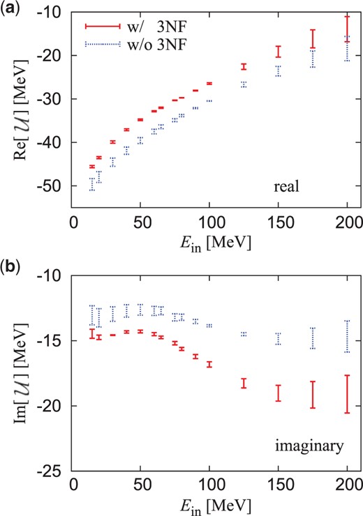
Single-particle potential |${\cal U}$| as a function of |$E_{\rm in}$| at |$k_{\rm F}=1.2$| fm|$^{-1}$| for the two cases of |$\Lambda=450, 550$| MeV. |$\Lambda$| dependence is shown as an error bar. The error bar plotted by a solid (dashed) line means the results of BHF calculations with (without) chiral 3NFs. Panels (a) and (b) show the real and imaginary parts of |${\cal U}$|⁠, respectively.

In order to obtain a deeper understanding of the properties of chiral 3NFs, we classify |$\tilde{g}(k_{\rm F},E_{\rm in})$| with total spin |$S$| and isospin |$T$| for the interacting two-nucleon system. The total single-particle potential |${\cal U}$| is obtained by the single-particle potential |${\cal U}^{ST}$| in each |$(S,T)$| channel as

\begin{eqnarray} {\cal U}=\sum_{ST}(2S+1)(2T+1){\cal U}^{ST}\!, \end{eqnarray}

(8)

where |${\cal U}^{ST}$| is defined by Eq. (6) with |$\tilde{g}$| replaced by |$\tilde{g}^{ST}$|⁠.

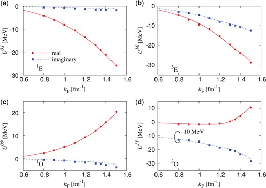
Figure 4 shows the |$E_{\rm in}$| dependence of |$U^{ST}\equiv (2S+1)(2T+1){\cal U}^{ST}$| for the case of |$k_{\rm F}=1.2$| fm|$^{-1}$|⁠. Here we perform the following three kinds of BHF calculations:

Fig. 4.

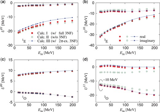
|$E_{\rm in}$| dependence of |$U^{ST} \equiv (2S+1)(2T+1){\cal U}^{ST}$| at |$k_{\rm F}=1.2$| fm|$^{-1}$| for (a) |$^{1}$|E (⁠|$S=0,T=1$|⁠), (b) |$^{3}$|E (⁠|$S=1,T=0$|⁠), (c) |$^{1}$|O (⁠|$S=0,T=0$|⁠), and (d) |$^{3}$|O (⁠|$S=1,T=1$|⁠). The filled circles (squares) represent |$U^{ST}$| in its real (imaginary) part obtained by BHF calculations with all kinds of chiral 3NFs. The open circles (squares) correspond to the real (imaginary) part of |$U^{ST}$| in which all kinds of chiral 3NFs are switched off. The lines with small circles (squares) stand for |$U^{ST}$| obtained by BHF calculations with |$c_D=c_E=0$|⁠. Note that the lines are a guide to the eye; the solid (dashed) line corresponds to the real (imaginary) part. For |$^{3}$|O, the imaginary part is shifted down by 10 MeV.

• I. All kinds of chiral 3NFs, i.e., diagrams (a)–(c) in Fig. 1, are taken into account.

• II. All kinds of chiral 3NFs are switched off. Namely, only chiral 2NF is considered.

• III. Diagrams (b) and (c) are ignored by setting |$c_D=c_E=0$| in BHF calculations. Namely, only the Fujita–Miyazawa 2|$\pi$|-exchange 3NF of diagram (a) is considered.

Filled circles (squares) stand for the real (imaginary) part of |$U^{ST}$| for calculation I, while open circles (squares) correspond to the real (imaginary) part of |$U^{ST}$| for calculation II; note that the lines are a guide to the eye. The two calculations show that chiral 3NF effects are significant for the |$^{3}$|O (⁠|$S=1,T=1$|⁠) and |$^{3}$|E (⁠|$S=1,T=0$|⁠) channel and the real part of the |$^{1}$|E (⁠|$S=0,T=1$|⁠) channel. The small circles (squares) represent the real (imaginary) part of |$U^{ST}$| for calculation III. For |$^{3}$|E and |$^{3}$|O, one can see from calculations II and III that chiral 3NF effects mainly come from the Fujita–Miyazawa 2|$\pi$|-exchange 3NF of diagram (a). For the real part of the |$^{1}$|E (⁠|$S=0,T=1$|⁠) channel, the effect of diagram (a) is sizable, but it is considerably reduced by the effects of diagrams (b) and (c). As a net effect of these properties, chiral 3NFs make |${\cal U}$| less attractive and more absorptive; the repulsion mainly stems from diagram (a) in its |$^{3}$|O component, and the absorption does from diagram (a) in its |$^{3}$|O and |$^{3}$|E components. The chiral-3NF effects become more significant at larger incident energies. One can easily expect that these properties also persist in the optical potentials of |$^{4}$|He scattering, since |${\cal U}$| plays the role of “optical potential” of nucleon scattering in nuclear matter. This point will be discussed later in Sect. 3.

2.3. Local version of chiral |$g$| matrix

The |$\tilde{g}$| matrix |$\tilde{g}(k_{\rm F},E_{\rm in})$| of Eq. (7) is a nonlocal potential depending on |$k_{\rm F}$| and |$E_{\rm in}$|⁠, being calculated in symmetric nuclear matter. In addition, it is obtained numerically. These properties are quite inconvenient in various applications. In order to circumvent the problem, the Melbourne group showed that elastic scattering is determined by the on-shell and near-on-shell components of the |$g$| matrix [24], and provided a local version of the |$g$| matrix in which the potential parameters are so determined as to reproduce the relevant components [24,37,38]. The Melbourne |$g$| matrix thus obtained accounts well for NN scattering in free space corresponding to the limit of |$\rho=0$|⁠, and the Melbourne |$g$|-matrix folding model reproduces NA scattering, as already mentioned in Sect. 1.

In our previous paper [28], following the Melbourne-group procedure [24,37,38], we succeeded in parameterizing a local version of the chiral |$\tilde{g}$| matrix in a three-range Gaussian form for each of the central, spin-orbit, and tensor components. The Gaussian form makes various kinds of numerical calculations efficient. The range and strength parameters were so determined as to reproduce the on-shell and near-on-shell matrix elements of the original |$\tilde{g}$| matrix for each spin–isospin channel, |$k_{\rm F}$| and |$E_{\rm in}$|⁠. As for the central part, the range parameters obtained were |$(0.4,0.9,2.5)$| in units of fm. In this paper, we repeated this procedure for |$E_{\rm in}$| up to 200 MeV and parameterized a local version of the chiral |$\tilde{g}$| matrix with good accuracy, as shown below. Since the analysis was already made at |$E_{\rm in}=65$| MeV in Ref. [28], we make the same analysis for higher energies, say |$E_{\rm in}=150$| MeV, in this paper. Whenever we have to distinguish the two types of |$g$| matrices, we call the local version of the |$\tilde{g}$| matrix the “Kyushu chiral |$g$| matrix” and the original nonlocal |$\tilde{g}$| matrix the “original chiral |$g$| matrix.” For the case of |$E_{\rm in}=75$| MeV as an example, we present the parameter set of the Kyushu chiral |$g$| matrix in Appendix A.

Figure 5 shows differential cross sections as a function of the c.m. scattering angle |$\theta_{\rm c.m.}$| for |$p$|+|$n$| scattering at |$E_{\rm in } =150$| MeV in free space, i.e., in the limit of |$\rho=0$|⁠. The solid and dashed lines denote the results of the original and Kyushu chiral |$t$| matrices, respectively; note that the |$g$| matrix is reduced to the |$t$| matrix in the limit of |$\rho=0$|⁠. The Kyushu chiral |$t$| matrix reproduces the result of the original chiral |$t$| matrix well.

Fig. 5.

Differential cross sections for |$p$|+|$n$| scattering at |$E_{\rm in } = 150$| MeV in free space. Here, |$\theta_{\rm c.m.}$| denotes the scattering angle in the center of mass system. The solid line stands for the result of the original chiral |$t$| matrix, while the dashed line corresponds to the result of the Kyushu chiral |$t$| matrix (the local version of chiral |$t$| matrix). Experimental data are taken from Ref. [39].

Figure 6 shows teh |$k_{\rm F}$| dependence of |$U^{ST}$| at |$E_{\rm in}=150$| MeV. Both 2NF and 3NF are taken into account in BHF calculations. The filled circles (squares) denote the results of the real (imaginary) part of the original chiral |$g$| matrix, whereas the solid (dashed) lines correspond to the real (imaginary) part of the Kyushu chiral |$g$| matrix. The range |$k_{\rm F} \underset{\raise0.3em\hbox{$\smash{\scriptscriptstyle\thicksim}$}}{<} 1.35$| fm|$^{-1}$| (⁠|$\rho \underset{\raise0.3em\hbox{$\smash{\scriptscriptstyle\thicksim}$}}{<} \rho_0$|⁠) contributes to the optical potentials of |$^{4}$|He scattering, when the potentials are constructed by the folding model explained in Sect. 2.4. In particular, the Fermi momentum |$k_{\rm F} \approx 1.2$| fm|$^{-1}$|⁠, corresponding to the peripheral region of the optical potentials, is important for elastic scattering. The Kyushu chiral |$g$| matrix reproduces well the results of the original chiral |$g$| matrix.

Fig. 6.

|$k_{\rm F}$| dependence of |$U^{ST}$| at |$E_{\rm in}=150$| MeV for (a) |$^{1}$|E, (b) |$^{3}$|E, (c) |$^{1}$|O, and (d) |$^{3}$|O. Here, 3NFs are taken into account in the BHF calculations. The filled circles (squares) stand for the results of the real (imaginary) part of the original chiral |$g$| matrix, while the solid (dashed) lines correspond to the results of the real (imaginary) part of the Kyushu chiral |$g$| matrix. For |$^{3}$|O, the imaginary part is shifted down by 10 MeV.

2.4. Folding model

In this paper, the optical potentials are derived by folding the Kyushu chiral |$g$| matrix with |$\rho_{\rm P}$| and |$\rho_{\rm T}$| for |$^{4}$|He scattering on |$^{208}$|Pb, |$^{58}$|Ni, and |$^{40}$|Ca targets. In general, the folding potential is referred to as a double-folding (DF) model for AA scattering, while it is called a single-folding (SF) model for NA scattering.

In the |$g$|-matrix SF model for NA elastic scattering, the so-called local-density approximation is taken; that is, the value of |$\rho$| in |$g(\rho)$| is identified with the value of |$\rho_{\rm T}$| at the midpoint |${\boldsymbol{r}}_{\rm m}$| of the two interacting nucleons: |$\rho=\rho_{\rm T}({\boldsymbol{r}}_{\rm m})$|⁠. Target-excitation effects on the elastic scattering are taken into account well by this framework. In fact, the Melbourne |$g$|-matrix SF model succeeded in reproducing NA scattering [24]. Furthermore, in our previous work [28] we showed that the Kyushu chiral |$g$|-matrix SF model also accounts well for proton scattering at |$E_{\rm in}=65$| MeV, and chiral-3NF effects are small there.

The |$g$|-matrix DF model for AA scattering had a problem to be settled. In order to obtain the |$g$| matrix applicable for AA scattering, in principle we have to consider two Fermi spheres in nuclear-matter calculations and solve a collision between a nucleon in the first Fermi sphere and a nucleon in the second one [40,41]. However, the actual calculations are not feasible. In fact, all the |$g$| matrices provided so far were obtained by assuming a single Fermi sphere and solving nucleon scattering on the Fermi sphere. For consistency with the nuclear-matter calculation, we assumed |$\rho=\rho_{\rm T}({\boldsymbol{r}}_{\rm m})$| in |$g(\rho)$| and applied the framework to |$^{3,4}$|He scattering in a wide energy range of |$30 \underset{\raise0.3em\hbox{$\smash{\scriptscriptstyle\thicksim}$}}{<} E_{\rm in}/A_{\rm P} \underset{\raise0.3em\hbox{$\smash{\scriptscriptstyle\thicksim}$}}{<} 180$| MeV [32,34]. The Melbourne |$g$|-matrix DF model based on the target-density approximation (TDA) accounted well for |$^{3,4}$|He scattering, particularly for forward differential cross sections where 3NF effects are considered to be negligible [25,26,29]. In our previous analysis [28], the DF-TDA model based on the Kyushu chiral |$g$| matrix explained well |$^{4}$|He scattering at |$E_{\rm in}/A_{\rm P} \approx 72$| MeV. We then take the DF-TDA model for |$^{4}$|He scattering in this paper throughout all the incident energies |$30 \underset{\raise0.3em\hbox{$\smash{\scriptscriptstyle\thicksim}$}}{<} E_{\rm in}/A_{\rm P} \underset{\raise0.3em\hbox{$\smash{\scriptscriptstyle\thicksim}$}}{<} 180$| MeV where experimental data are available.

The DF model naturally treats both the direct and knock-on exchange processes [41–43]. In the latter process, two interacting nucleons are exchanged and thereby the potential becomes nonlocal. However, the nonlocality can be localized with high accuracy by the local momentum approximation [21–23], as proven in Refs. [44,45]. The folding potential |$U(R)$| thus obtained is a function of the distance |$R$| between P and T:

\begin{eqnarray} U(R)&&= \sum_{\mu\nu}\int d{\boldsymbol{r}}_{\rm P} \int d{\boldsymbol{r}}_{\rm T}&&&&& \rho_{\rm P}^{(\mu)}(r_{\rm P})\rho_{\rm T}^{(\nu)}(r_{\rm T}) \tilde{g}^{\rm DR}_{\mu\nu}(s,E_{\rm in}/A_{\rm P};\rho) \nonumber\\ &&\quad{} -\sum_{\mu\nu}\int d{\boldsymbol{r}}_{\rm P} \int d{\boldsymbol{r}}_{\rm T}&&&&& \tilde{\rho}_{\rm P}^{(\mu)}({\boldsymbol{r}}_{\rm P},{\boldsymbol{s}}) \tilde{\rho}_{\rm T}^{(\nu)}({\boldsymbol{r}}_{\rm T},{\boldsymbol{s}}) \tilde{g}^{\rm EX}_{\mu\nu}(s,E_{\rm in}/A_{\rm P};\rho) j_{0}({\scriptstyle \frac{A_{\rm P}+A_{\rm T}}{A_{\rm P}A_{\rm T}}}K(R)s), \end{eqnarray}

(9)

where the indices |$\mu$| and |$\nu$| are the isospins of the corresponding nucleons and |${\boldsymbol{s}}= {\boldsymbol{r}}_{\rm T}-{\boldsymbol{r}}_{\rm P}-{\boldsymbol{R}}$| is the coordinate between the two interacting nucleons. The densities |$\rho_{\rm P(T)}$| and |$\tilde{\rho}_{\rm P(T)}$| represent the one-body and mixed densities of P (T):

\begin{eqnarray} \tilde{\rho}_{\rm P(T)}&=& \rho_{\rm P(T)}(|{\boldsymbol{r}}_{\rm P(T)}\pm {\boldsymbol{s}}/2|) \frac{3j_{1}(k_{\rm F}^{\rm P(T)}s)}{k_{\rm F}^{\rm P(T)}s}. \end{eqnarray}

(10)

The Fermi momentum |$k_{\rm F}^{\rm P(T)}$| is related to the density |$\rho_{\rm P(T)}$|⁠. The direct (exchange) term of the |$g$|-matrix |$\tilde{g}^{\rm DR(EX)}_{\mu \nu}$| is defined by |$\tilde{g}^{ST}$| as

\begin{eqnarray} \tilde{g}^{\rm DR(EX)}_{pp,nn} &=&\frac{1}{4}(\pm \tilde{g}^{01}+3\tilde{g}^{11}), \end{eqnarray}

(11)

\begin{eqnarray} \tilde{g}^{\rm DR(EX)}_{pn,np} &=&\frac{1}{8}(\tilde{g}^{00}\pm \tilde{g}^{01} \pm 3\tilde{g}^{10} + 3\tilde{g}^{11}). \end{eqnarray}

(12)

See Refs. [29,34,46,47] for the details of the formulation of the DF model. The |$S$| matrices for |$^{4}$|He elastic scattering are obtained by solving the one-body Schrödinger equation with |$U(R)$|⁠.

For the targets |$^{208}$|Pb and |$^{58}$|Ni, the matter densities |$\rho_{\rm T}$| are evaluated by the spherical Hartree–Fock (HF) method based on the Gogny-D1S interaction [48], where the spurious c.m. motions are removed in the standard manner [49]. For the projectile |$^{4}$|He and the target |$^{40}$|Ca, we take the phenomenological proton density determined from electron scattering [50]; here, the finite-size effect of proton charge is unfolded with the standard procedure [51], and the neutron density is assumed to have the same geometry as the proton one, since the difference between the neutron root-mean-square radius and the proton one is only 1% in spherical HF calculations.

3. Results

Now we analyze |$^{4}$|He elastic scattering on nuclei systematically for a wide range of |$E_{\rm in}/A_{\rm P}=26$|–|$175$| MeV. Here, the heavier targets |$^{208}$|Pb, |$^{58}$|Ni, and |$^{40}$|Ca are considered, because the |$g$| matrix is calculated in nuclear matter and the |$g$|-matrix DF model is expected to be more reliable for heavier targets.

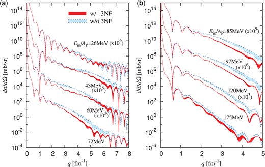
Figure 7 shows differential cross sections |$d \sigma/d \Omega$| as a function of transfer momentum |$q$| for |$^{4}$|He scattering from a |$^{208}$|Pb target for |$E_{\rm in}/A_{\rm P}=26$|–|$175$| MeV where the experimental data are available. The solid and dashed lines stand for the results of the Kyushu chiral |$g$|-matrix DF model with and without 3NF effects, respectively. Chiral 3NFs improve the agreement of the theoretical results with the experimental data. Particularly for |$E_{\rm in}/A_{\rm P} \underset{\raise0.3em\hbox{$\smash{\scriptscriptstyle\thicksim}$}}{>} 100$| MeV, the agreement is pretty good. We can also observe the same features for |$^{58}$|Ni and |$^{40}$|Ca targets, as shown in Figs. 8 and 9, although there is a tendency that the agreement becomes better as the target mass increases.

Fig. 7.

Differential cross sections |$d \sigma/d \Omega$| as a function of transfer momentum |$q$| for |$^{4}$|He scattering from a |$^{208}$|Pb target at |$E_{\rm in}/A_{\rm P}=26$|–|$175$| MeV. The solid (dashed) lines denote the results of the Kyushu chiral |$g$| matrix with (without) 3NF effects. Each cross section is multiplied by the factor shown in the figure. Experimental data are taken from Refs. [52–55].

Fig. 8.

As Fig. 7, but the target nucleus is |$^{58}$|Ni. Experimental data are taken from Refs. [54,56–60].

Fig. 9.

As Fig. 7, but the target nucleus is |$^{40}$|Ca. Experimental data are taken from Refs. [52,61,62].

Now we analyze the effects of the Fujita–Miyazawa 2|$\pi$|-exchange 3NF on differential cross sections |$d \sigma/d \Omega$| for |$^{4}$|He+|$^{58}$|Ni scattering. In Fig. 10, the solid, dashed, and dot-dashed lines denote the results of calculations I, II, and III, respectively; see Sect. 2.2 for the definitions of the |$g$|-matrix calculations. The difference between calculations I and II means effects of all 3NFs, and that between calculations II and III corresponds to effects of the Fujita–Miyazawa 2|$\pi$|-exchange 3NF. The resultant cross sections show that the Fujita–Miyazawa 2|$\pi$|-exchange 3NF is the main contribution of chiral-3NF effects on |$^{4}$|He scattering.

Fig. 10.

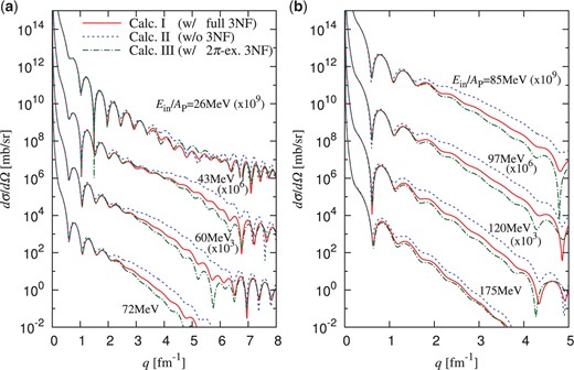
Effects of Fujita–Miyazawa 2|$\pi$|-exchange 3NF on differential cross sections |$d \sigma/d \Omega$| for |$^{4}$|He+|$^{58}$|Ni scattering, where |$q$| is the transfer momentum. The solid and dashed lines denote the results of calculations I and II, respectively, and the dot-dashed line corresponds to the results of calculation III; see Sect. 2.2 for the definitions of the |$g$|-matrix calculations. Each cross section is multiplied by the factor shown in the figure.

Figure 11 shows the |$R$| dependence of the optical potentials |$U(R)$| for |$^{4}$|He elastic scattering from a |$^{58}$|Ni target at |$E_{\rm in}/A_{\rm P}=$|26, 60, and 175 MeV. The solid and dashed lines represent the |$U(R)$| with and without chiral-3NF effects; note that only the central potential is generated by the DF-TDA model. As expected, chiral-3NF effects make repulsive and absorptive corrections to the optical potentials, and the corrections slightly increase as |$E_{\rm in}$| increases; note that the effects hardly depend on |$E_{\rm in}$| in the peripheral region, |$R \approx 6$| fm, which is important for the elastic scattering. As already mentioned in Sect. 2.2, the repulsive correction mainly comes from the Fujita–Miyazawa 2|$\pi$|-exchange 3NF in its |$^{3}$|O component, and the absorptive correction stems from the |$^{3}$|E and |$^{3}$|O components of the Fujita–Miyazawa 2|$\pi$|-exchange 3NF.

Fig. 11.

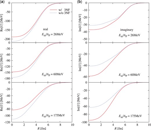
Optical potentials |$U(R)$| as a function of |$R$| for |$^{4}$|He+|$^{58}$|Ni elastic scattering at |$E_{\rm in}/A_{\rm P}=$|26, 60, and 175 MeV. The solid (dashed) lines denote the optical potentials with (without) chiral-3NF effects. Panels (a) and (b) represent the real and imaginary parts of |$U$|⁠, respectively.

Figure 12 shows the uncertainty coming from the |$\Lambda$| dependence of the differential cross sections |$d \sigma/d \Omega$| for |$^{4}$|He+|$^{58}$|Ni elastic scattering. Here, two cases of |$\Lambda=550$| and |$450$| MeV are considered. The |$\Lambda$| dependence is shown by hatching for each of the 2NF and 2NF+3NF calculations; note that the hatched region surrounded by solid (dashed) lines means the uncertainty coming from |$\Lambda$| dependence for 2NF+3NF (2NF) calculations. As expected, |$\Lambda$| dependence becomes larger as |$E_{\rm in}$| increases, but the uncertainty coming from |$\Lambda$| dependence is still smaller than the chiral-3NF effects, even at |$E_{\rm in}/A_{\rm P}=175$| MeV.

Fig. 12.

Uncertainty coming from |$\Lambda$| dependence of differential cross sections |$d \sigma/d \Omega$| for |$^{4}$|He+|$^{58}$|Ni elastic scattering. |$\Lambda$| dependence is indicated by hatching for each of the 2NF and 2NF+3NF calculations, where two cases of |$\Lambda=550$| and |$450$| MeV are taken. Note that the hatched region surrounded by the solid (dashed) lines corresponds to the uncertainty coming from |$\Lambda$| dependence for 2NF+3NF (2NF) calculations.

The scattering amplitude can be decomposed into near- and far-side components [63]. As illustrated in Fig. 13, these components are well defined when outgoing waves are generated only in the peripheral region of T. |$^{4}$|He scattering on a heavier target is a good case. The absorptive correction of chiral-3NF effects makes the decomposition more applicable. The decomposition is a convenient tool for investigating the interplay between differential cross sections |$d \sigma/d \Omega$| and the real part of |$U(R)$|⁠. The near-side (far-side) outgoing waves are mainly induced by the repulsive Coulomb (attractive nuclear) force, so that very-forward-angle (middle-angle) scattering is dominated by the near-side (far-side) components. As a consequence of this property, a large interference pattern appears in the differential cross sections at the forward angles where the two components become comparable, and the far-side dominance is realized at middle angles after the interference pattern. In the middle-angle region, any repulsive correction to |$U(R)$| reduces the differential cross sections.

Fig. 13.

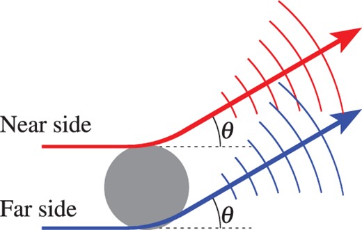
Illustration of near/far decomposition.

Figure 14 shows the near/far decomposition of the differential cross sections |$d \sigma/d \Omega$| for |$^{4}$|He+|$^{58}$|Ni scattering at |$E_{\rm in }/A_{\rm P} = 72$| MeV. The dotted and dashed lines represent the near- and far-side cross sections, respectively, and the solid line denotes differential cross sections before the near/far decomposition; here, chiral-3NF effects are taken into account. The solid line shows a large interference pattern at |$\theta_{\rm c.m.}= 5$|–|$15^\circ$|⁠, and the solid line agrees with the dashed one for |$20^\circ \underset{\raise0.3em\hbox{$\smash{\scriptscriptstyle\thicksim}$}}{<} \theta_{\rm c.m.} \underset{\raise0.3em\hbox{$\smash{\scriptscriptstyle\thicksim}$}}{<} 40^\circ$|⁠. The far-side dominance is thus realized for middle angles |$20^\circ \underset{\raise0.3em\hbox{$\smash{\scriptscriptstyle\thicksim}$}}{<} \theta_{\rm c.m.} \underset{\raise0.3em\hbox{$\smash{\scriptscriptstyle\thicksim}$}}{<} 40^\circ$|⁠. The far-side dominance for |$20^\circ \underset{\raise0.3em\hbox{$\smash{\scriptscriptstyle\thicksim}$}}{<} \theta_{\rm c.m.} \underset{\raise0.3em\hbox{$\smash{\scriptscriptstyle\thicksim}$}}{<} 40^\circ$| persists, even after chiral 3NFs are switched off. The dot-dashed line is the far-side cross section in which chiral 3NFs are switched off. The repulsive correction coming from chiral 3NFs suppresses the differential cross sections for far-side dominant angles |$20^\circ \underset{\raise0.3em\hbox{$\smash{\scriptscriptstyle\thicksim}$}}{<} \theta_{\rm c.m.} \underset{\raise0.3em\hbox{$\smash{\scriptscriptstyle\thicksim}$}}{<} 40^\circ$| from the dot-dashed line to the solid (dashed) line. Thus, chiral-3NF effects become more visible in the far-side dominant angle region.

Fig. 14.

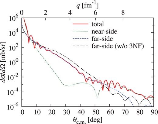
Near/far decomposition of differential cross sections |$d \sigma/d \Omega$| for |$^{4}$|He+|$^{58}$|Ni scattering at |$E_{\rm in }/A_{\rm P} = 72$| MeV. The dotted (dashed) line stands for the near-side (far-side) cross sections, while the solid line denotes differential cross sections before the near/far decomposition; here, chiral-3NF effects are taken into account. The dot-dashed line corresponds to the far-side cross section in which chiral 3NFs are switched off.

Finally, we briefly comment on chiral-3NF effects on total reaction cross sections |$\sigma_{\rm R}$|⁠. Radii of stable and unstable nuclei are often determined from measured |$\sigma_{\rm R}$| with the folding model and/or the Glauber model. Figure 15 shows |$\sigma_{\rm R}$| as a function of |$E_{\rm in}/A_{\rm P}$| for |$^{4}$|He scattering on |$^{58}$|Ni and |$^{208}$|Pb targets. The closed circles (squares) represent the results of the Kyushu chiral |$g$| matrix with (without) 3NF effects. The two kinds of results are close to each other, indicating that chiral-3NF effects are negligible for |$\sigma_{\rm R}$|⁠. This fact ensures that the determination of nuclear radii from measured |$\sigma_{\rm R}$| is reliable.

Fig. 15.

Total reaction cross sections |$\sigma_{\rm R}$| as a function of |$E_{\rm in}$| for |$^{4}$|He scattering on (a) |$^{58}$|Ni and (b) |$^{58}$|Pb targets. Closed circles (squares) denote the results of the Kyushu chiral |$g$| matrix with (without) 3NF effects. Experimental data are taken from Refs. [54,64].

4. Summary

Wen have investigated the basic properties of chiral 3NFs in symmetric nuclear matter with positive energies up to 200 MeV by using the BHF method with chiral 2NFs of N|$^{3}$|LO and chiral 3NFs of NNLO in the Bochum–Bonn–Jölich [36] parameterization, and analyzed chiral-3NF effects on |$^{4}$|He elastic scattering from heavier targets |$^{208}$|Pb, |$^{58}$|Ni, and |$^{40}$|Ca over a wide incident-energy range of |$30 \underset{\raise0.3em\hbox{$\smash{\scriptscriptstyle\thicksim}$}}{<} E_{\rm in}/A_{\rm P} \underset{\raise0.3em\hbox{$\smash{\scriptscriptstyle\thicksim}$}}{<} 200$| MeV by the Kyushu chiral |$g$|-matrix folding model.

First, we summarize the basic properties of chiral 3NFs in symmetric nuclear matter with positive energies |$E_{\rm in}$| up to 200 MeV:

• (1) Chiral 3NFs make the single-particle potential |${\cal U}$| less attractive and more absorptive.

• (2) The repulsive and absorptive corrections slightly increase as |$E_{\rm in}$| goes up.

• (3) Chiral 3NF effects on |${\cal U}$| mainly come from the Fujita–Miyazawa 2|$\pi$|-exchange 3NF [Fig. 1(a)]. More precisely, the repulsion mainly stems from the |$^{3}$|O component of Fig. 1(a) and the absorption comes from the |$^{3}$|O and |$^{3}$|E components of Fig. 1(a).

Properties (1)–(3) persist in the optical potential of |$^{4}$|He scattering. This is natural, since the single-particle potential plays the role of the optical potential in nuclear matter. However, it should be noted that chiral-3NF effects depend little on |$E_{\rm in}$| in the peripheral region that is important for the elastic scattering.

Chiral-3NF effects are evident for |$^{4}$|He scattering for |$E_{\rm in}/A_{\rm P} \underset{\raise0.3em\hbox{$\smash{\scriptscriptstyle\thicksim}$}}{>} 60$| MeV at the middle angles where the cross sections are dominated by the far-side component of the scattering amplitude. The repulsive correction of chiral 3NFs reduces the far-side component and thereby yields better agreement with the experimental data. Eventually, the Kyushu chiral |$g$|-matrix DF model reproduces measured differential cross sections pretty well, particularly for |$^{4}$|He scattering at |$E_{\rm in}/A_{\rm P} \underset{\raise0.3em\hbox{$\smash{\scriptscriptstyle\thicksim}$}}{>} 100$| MeV.

All the analyses mentioned above were made with |$\Lambda=550$| MeV. In order to investigate |$\Lambda$| dependence in nuclear-matter and |$^{4}$|He-scattering calculations, we took |$\Lambda=450$| MeV in addition to |$\Lambda=550$| MeV. The uncertainty coming from |$\Lambda$| dependence is smaller than the chiral-3NF effects. There is a tendency that the uncertainty becomes larger as |$E_{\rm in}$| increases, but it is still smaller than the chiral-3NF effects even at |$E_{\rm in} = 175$| MeV.

Finally, we provided the local version of the chiral |$g$|-matrix with a three-range Gaussian form for the case of |$E_{\rm in}=72$| MeV. Numerical values are presented in Appendix A. This local version of the chiral |$g$| matrix strongly encourages us to use it for studying various kinds of nuclear reactions.

Acknowledgments

The authors would like to thank K. Ogata and K. Minomo for valuable discussions on localization of the chiral |$g$|-matrix and the reaction analyses. This work is supported in part by by Grants-in-Aid for Scientific Research (Nos. 25400266, 26400278, 16K05353, and 16J00630) from the Japan Society for the Promotion of Science (JSPS).

Appendix A. Parameter set of the Kyushu chiral |$g$| matrix

In this Appendix we provide the central part of the Kyushu chiral |$g$| matrix for the case of |$E_{\rm in}/A_{\rm P}=75$| MeV in a three-range Gaussian form,

\begin{eqnarray} g^{ST}(s,k_{\rm F},E_{\rm in}/A_{\rm P}) =\sum_{i=1}^{3} g^{ST}_{i}(k_{\rm F},E_{\rm in}/A_{\rm P}) e^{-s^2/\lambda_i^2} , \end{eqnarray}

(A.1)

in each |$(S, T)$| channel. The range parameters are fixed to be |$(\lambda_1,\lambda_2,\lambda_3)=(0.4, 0.9, 2.5)$| in units of fm, and the strength parameters |$\tilde{g}^{ST}_{i}(k_{\rm F},E_{\rm in}/A_{\rm P})$| in units of MeV, which include chiral 3NF effects, are tabulated in Tables A1–A4 for six cases of the Fermi momentum |$k_{\rm F}$|⁠. We will make the parameter sets of other cases available electronically [65].

Table A1

Singlet-even (⁠|$S=0,T=1$|⁠) component of the Kyushu chiral |$g$| matrix for the incident energy |$E_{\rm in}/A_{\rm P}=75$| MeV. The range parameters are fixed to be |$(\lambda_1,\lambda_2,\lambda_3)=(0.4, 0.9, 2.5)$| in units of fm. Entries are in MeV, but |$k_{\rm F}$| is presented in units of fm|$^{-1}$|⁠.

		Real part				Imaginary part
|$k_{\rm F}$|		|$i=1$|	|$i=2$|	|$i=3$|		|$i=1$|	|$i=2$|	|$i=3$|
|$0.00$|		1.78627|$\times 10^{3}$|	|$-$|2.70833|$\times 10^{2}$|	|$-$|4.08777|$\times 10^{0}$|		2.16654|$\times 10^{3}$|	|$-$|3.13038|$\times 10^{2}$|	1.39295|$\times 10^{0}$|
|$0.60$|		1.47941|$\times 10^{3}$|	|$-$|2.47638|$\times 10^{2}$|	|$-$|3.68242|$\times 10^{0}$|		1.13963|$\times 10^{3}$|	|$-$|1.71777|$\times 10^{2}$|	8.14716|$\times 10^{-1}$|
|$0.80$|		1.36782|$\times 10^{3}$|	|$-$|2.39203|$\times 10^{2}$|	|$-$|3.53502|$\times 10^{0}$|		7.66206|$\times 10^{2}$|	|$-$|1.20410|$\times 10^{2}$|	6.04451|$\times 10^{-1}$|
|$1.10$|		1.20044|$\times 10^{3}$|	|$-$|2.26551|$\times 10^{2}$|	|$-$|3.31392|$\times 10^{0}$|		2.06075|$\times 10^{2}$|	|$-$|4.33587|$\times 10^{1}$|	2.89052|$\times 10^{-1}$|
|$1.20$|		1.09716|$\times 10^{3}$|	|$-$|2.13700|$\times 10^{2}$|	|$-$|3.19454|$\times 10^{0}$|		1.25689|$\times 10^{2}$|	|$-$|2.88651|$\times 10^{1}$|	1.74997|$\times 10^{-1}$|
|$1.30$|		9.54436|$\times 10^{2}$|	|$-$|1.94839|$\times 10^{2}$|	|$-$|3.14638|$\times 10^{0}$|		6.90248|$\times 10^{1}$|	|$-$|1.93121|$\times 10^{1}$|	9.44602|$\times 10^{-2}$|
|$1.40$|		7.65583|$\times 10^{2}$|	|$-$|1.68406|$\times 10^{2}$|	|$-$|3.19684|$\times 10^{0}$|		1.85011|$\times 10^{1}$|	|$-$|1.05755|$\times 10^{1}$|	2.29847|$\times 10^{-2}$|
|$1.50$|		5.88265|$\times 10^{2}$|	|$-$|1.44596|$\times 10^{2}$|	|$-$|3.21499|$\times 10^{0}$|		|$-$|1.57455|$\times 10^{0}$|	|$-$|7.13793|$\times 10^{0}$|	|$-$|1.93808|$\times 10^{-3}$|

Table A2

Triplet-even (⁠|$S=1,T=0$|⁠) component of the Kyushu chiral |$g$| matrix for the incident energy |$E_{\rm in}/A_{\rm P}=75$| MeV. See Table A1 for the detail.

		Real part				Imaginary part
|$k_{\rm F}$|		|$i=1$|	|$i=2$|	|$i=3$|		|$i=1$|	|$i=2$|	|$i=3$|
|$0.00$|		1.25135|$\times 10^{3}$|	|$-$|2.14233|$\times 10^{2}$|	|$-$|4.23044|$\times 10^{0}$|		2.83713|$\times 10^{3}$|	|$-$|4.39936|$\times 10^{2}$|	|$-$|7.11017|$\times 10^{-1}$|
|$0.60$|		1.26094|$\times 10^{3}$|	|$-$|2.62345|$\times 10^{2}$|	|$-$|3.04629|$\times 10^{0}$|		1.96817|$\times 10^{3}$|	|$-$|3.18594|$\times 10^{2}$|	|$-$|4.36898|$\times 10^{-1}$|
|$0.80$|		1.26443|$\times 10^{3}$|	|$-$|2.79841|$\times 10^{2}$|	|$-$|2.61569|$\times 10^{0}$|		1.65218|$\times 10^{3}$|	|$-$|2.74470|$\times 10^{2}$|	|$-$|3.37218|$\times 10^{-1}$|
|$1.10$|		1.26966|$\times 10^{3}$|	|$-$|3.06084|$\times 10^{2}$|	|$-$|1.96978|$\times 10^{0}$|		1.17821|$\times 10^{3}$|	|$-$|2.08284|$\times 10^{2}$|	|$-$|1.87698|$\times 10^{-1}$|
|$1.20$|		1.13634|$\times 10^{3}$|	|$-$|2.90035|$\times 10^{2}$|	|$-$|1.65944|$\times 10^{0}$|		9.55010|$\times 10^{2}$|	|$-$|1.67104|$\times 10^{2}$|	|$-$|3.11895|$\times 10^{-1}$|
|$1.30$|		9.50006|$\times 10^{2}$|	|$-$|2.63272|$\times 10^{2}$|	|$-$|1.57370|$\times 10^{0}$|		8.52716|$\times 10^{2}$|	|$-$|1.48093|$\times 10^{2}$|	|$-$|4.61621|$\times 10^{-1}$|
|$1.40$|		5.98320|$\times 10^{2}$|	|$-$|2.11212|$\times 10^{2}$|	|$-$|1.85361|$\times 10^{0}$|		8.38254|$\times 10^{2}$|	|$-$|1.45648|$\times 10^{2}$|	|$-$|5.53945|$\times 10^{-1}$|
|$1.50$|		4.87230|$\times 10^{2}$|	|$-$|1.95265|$\times 10^{2}$|	|$-$|1.99886|$\times 10^{0}$|		8.31225|$\times 10^{2}$|	|$-$|1.43294|$\times 10^{2}$|	|$-$|6.62903|$\times 10^{-1}$|

Table A3

Singlet-odd (⁠|$S=0,T=0$|⁠) component of the Kyushu chiral |$g$| matrix for the incident energy |$E_{\rm in}/A_{\rm P}=75$| MeV. See Table A1 for the detail.

		Real part				Imaginary part
|$k_{\rm F}$|		|$i=1$|	|$i=2$|	|$i=3$|		|$i=1$|	|$i=2$|	|$i=3$|
|$0.00$|		1.17797|$\times 10^{3}$|	1.54048|$\times 10^{1}$|	9.23703|$\times 10^{0}$|		6.01921|$\times 10^{2}$|	|$-$|6.69649|$\times 10^{1}$|	|$-$|3.21021|$\times 10^{-1}$|
|$0.60$|		2.92329|$\times 10^{2}$|	9.73676|$\times 10^{1}$|	8.54387|$\times 10^{0}$|		4.56013|$\times 10^{2}$|	|$-$|5.19773|$\times 10^{1}$|	|$-$|1.83729|$\times 10^{-1}$|
|$0.80$|		|$-$|2.97222|$\times 10^{1}$|	1.27172|$\times 10^{2}$|	8.29181|$\times 10^{0}$|		4.02955|$\times 10^{2}$|	|$-$|4.65273|$\times 10^{1}$|	|$-$|1.33805|$\times 10^{-1}$|
|$1.10$|		|$-$|5.12800|$\times 10^{2}$|	1.71879|$\times 10^{2}$|	7.91372|$\times 10^{0}$|		3.23369|$\times 10^{2}$|	|$-$|3.83522|$\times 10^{1}$|	|$-$|5.89192|$\times 10^{-2}$|
|$1.20$|		|$-$|6.98327|$\times 10^{2}$|	1.94038|$\times 10^{2}$|	7.80370|$\times 10^{0}$|		3.02061|$\times 10^{2}$|	|$-$|3.67462|$\times 10^{1}$|	|$-$|4.49149|$\times 10^{-2}$|
|$1.30$|		|$-$|8.68590|$\times 10^{2}$|	2.13672|$\times 10^{2}$|	7.65323|$\times 10^{0}$|		3.08332|$\times 10^{2}$|	|$-$|3.85626|$\times 10^{1}$|	|$-$|3.61166|$\times 10^{-2}$|
|$1.40$|		|$-$|1.21630|$\times 10^{3}$|	2.43679|$\times 10^{2}$|	7.28544|$\times 10^{0}$|		3.39578|$\times 10^{2}$|	|$-$|4.29750|$\times 10^{1}$|	|$-$|1.70789|$\times 10^{-2}$|
|$1.50$|		|$-$|1.35278|$\times 10^{3}$|	2.58695|$\times 10^{2}$|	7.07301|$\times 10^{0}$|		3.38596|$\times 10^{2}$|	|$-$|4.29790|$\times 10^{1}$|	|$-$|8.86515|$\times 10^{-3}$|

Table A4

Triplet-odd (⁠|$S=1,T=1$|⁠) component of the Kyushu chiral |$g$| matrix for the incident energy |$E_{\rm in}/A_{\rm P}=75$| MeV. See Table A1 for the detail.

		Real part				Imaginary part
|$k_{\rm F}$|		|$i=1$|	|$i=2$|	|$i=3$|		|$i=1$|	|$i=2$|	|$i=3$|
|$0.00$|		1.48087|$\times 10^{3}$|	|$-$|1.17015|$\times 10^{2}$|	4.09818|$\times 10^{-1}$|		6.26964|$\times 10^{2}$|	|$-$|5.48253|$\times 10^{1}$|	|$-$|2.34394|$\times 10^{-1}$|
|$0.60$|		9.89803|$\times 10^{2}$|	|$-$|7.76051|$\times 10^{1}$|	3.97949|$\times 10^{-1}$|		4.90110|$\times 10^{2}$|	|$-$|4.36088|$\times 10^{1}$|	|$-$|1.27683|$\times 10^{-1}$|
|$0.80$|		8.11232|$\times 10^{2}$|	|$-$|6.32740|$\times 10^{1}$|	3.93633|$\times 10^{-1}$|		4.40345|$\times 10^{2}$|	|$-$|3.95300|$\times 10^{1}$|	|$-$|8.88792|$\times 10^{-2}$|
|$1.10$|		5.43375|$\times 10^{2}$|	|$-$|4.17774|$\times 10^{1}$|	3.87159|$\times 10^{-1}$|		3.65697|$\times 10^{2}$|	|$-$|3.34119|$\times 10^{1}$|	|$-$|3.06733|$\times 10^{-2}$|
|$1.20$|		3.30284|$\times 10^{2}$|	|$-$|2.25888|$\times 10^{1}$|	3.93880|$\times 10^{-1}$|		3.57729|$\times 10^{2}$|	|$-$|3.29841|$\times 10^{1}$|	|$-$|1.48011|$\times 10^{-2}$|
|$1.30$|		1.31873|$\times 10^{2}$|	|$-$|4.61127|$\times 10^{0}$|	3.96357|$\times 10^{-1}$|		3.94174|$\times 10^{2}$|	|$-$|3.67176|$\times 10^{1}$|	|$-$|2.33502|$\times 10^{-3}$|
|$1.40$|		|$-$|9.73856|$\times 10^{1}$|	1.42601|$\times 10^{1}$|	3.20402|$\times 10^{-1}$|		4.67099|$\times 10^{2}$|	|$-$|4.37829|$\times 10^{1}$|	2.27706|$\times 10^{-2}$|
|$1.50$|		|$-$|2.46017|$\times 10^{2}$|	2.76700|$\times 10^{1}$|	3.11786|$\times 10^{-1}$|		5.04428|$\times 10^{2}$|	|$-$|4.77850|$\times 10^{1}$|	3.25825|$\times 10^{-2}$|