Path optimization in |$0+1$|D QCD at finite density

Abstract

We investigate the sign problem in |$0+1$|D quantum chromodynamics at finite chemical potential by using the path optimization method. The SU(3) link variable is complexified to the SL(3,|$\mathbb{C}$|⁠) link variable, and the integral path is represented by a feedforward neural network. The integral path is then optimized to weaken the sign problem. The average phase factor is enhanced to be greater than 0.99 on the optimized path. Results with and without diagonalized gauge fixing are compared and proven to be consistent. This is the first step in applying the path optimization method to gauge theories.

1. Introduction

Solving the sign problem for complex actions in the path integral is one of the grand challenges in theoretical physics. When the Boltzmann weight is a complex-valued highly oscillating function, the strong cancellation takes place and it is difficult to control the numerical error of integration. The sign problem is a generic problem in finite-density fermion systems such as finite-density quantum chromodynamics (QCD). There have been various approaches proposed so far to avoid or evade the sign problem in finite-density lattice QCD. These approaches include the reweighting method [1–4], the Taylor expansion method [5–7], the analytic continuation [8–12], and the canonical method by using the imaginary chemical potential [13–18], the density of states method [19,20], and strong coupling QCD [21–25]. Unfortunately, these methods work only in the region of |$\mu/T \lesssim 1$|⁠, with heavy quark mass, or in the strong coupling regime at present.

In addition, several approaches based on complexified variables have been developed, and have recently attracted much attention. It may be possible to discuss physics with a severe sign problem. These approaches include the complex Langevin method [26,27], the Lefschetz thimble method [28–30], and the path optimization method [31–34]. In this study, we use the path optimization method.

In the path optimization method, the integration path (or manifold) is prepared appropriately, and optimized so as to weaken the seriousness of the sign problem. The present authors have proposed this method [31], and have applied it to the 1D integral of a highly oscillating complex function [31], the 2D scalar field theory at finite density [32], and the Polyakov-loop extended Nambu–Jona-Lasinio model [33,34]. This method has also been applied to the Thirring model [35] and the 1D complex scalar field theory at finite density [36].

Now, it is important to discuss the sign problem in gauge theories by using the path optimization method. As the first step, we consider |$0+1$|D QCD. |$0+1$|D QCD has the sign problem at finite chemical potential, and the temporal hopping term of quarks is the origin of the sign problem, as in |$3+1$|D QCD, while we do not have the fake early onset problem of the baryon number in |$0+1$|D QCD. The analytic solution is known for |$0+1$|D QCD [37], so it is a good laboratory to examine the framework for the sign problem in gauge theory. Actually, |$0+1$|D QCD has been studied by using the complex Langevin method [38], the Lefschetz thimble method [39], the subset method [40,41], the polynomially exact integration method [42], and so on.

In this article, as the first step towards investigating the sign problem in gauge theories in |$3+1$| dimensions, we apply the path optimization method to |$0+1$|D QCD at finite chemical potential. We develop the method to complexify the SU(3) link variable to that in SL(3,|$\mathbb{C}$|⁠). The integral path is prepared by using a feedforward neural network, and is optimized to evade the sign problem. We have found that the average phase factor on the optimized path exceeds 0.99, which may allow us to study finite-density QCD at higher dimensions. We also compare the results with and without diagonalized gauge fixing, and the results are found to be consistent with each other.

This paper is organized as follows. In Sects. 2 and 3, we explain |$0+1$|D QCD and the path optimization method, respectively. We also discuss how to complexify the link variable. In Sect. 4, we show the results with and without diagonalized gauge fixing, and compare these results. In Sect. 5, we summarize this paper.

2. |$\boldsymbol{0+1}$|D QCD

In this study, we consider |$0+1$|D QCD at finite density with and without diagonalized gauge fixing in the path optimization method. Details are shown below.

2.1. Partition function and observables

The partition function of the |$0+1$|D QCD in the Euclidean spacetime is given as [37,43]

$$\begin{align} {\cal Z} &= \int \mathcal{D}\overline{\chi}\, \mathcal{D}\chi\, \mathcal{D}U ~ e^{-S[\chi, \overline{\chi},U]}, \label{eq:part_fn} \end{align}$$

(1)

with the lattice action

$$\begin{align} S &= \frac{1}{2} \sum^{N_\tau}_{\tau=1} (\overline{\chi}_\tau e^{\mu} U_\tau \chi_{\tau+1} - \overline{\chi}_{\tau+1} e^{-\mu} U^{-1}_\tau \chi_\tau) + m \sum_\tau \overline{\chi}_\tau\chi_\tau, \label{eq:action} \end{align}$$

(2)

where we consider one species of staggered fermion |$\chi$|⁠, |$U_\tau$| is the |$\mathrm{SU}(3)$| link variable in the temporal direction, |$m$| denotes the bare fermion mass, |$\mu$| is the chemical potential, and |$N_\tau$| is the number of lattice sites in the temporal direction. By using the gauge transformation, one can reduce the degree of freedom to one link variable, and the partition function is rewritten as

$$\begin{align} {\cal Z} =& \int dU\, \det D(U),\label{Eq:Z}\\ \end{align}$$

(3)

$$\begin{align} D(U) =&\, X + e^{\mu/T} U(\theta) + e^{-\mu /T}U^{-1}(\theta), \end{align}$$

(4)

where |$X = 2\cosh(E/T)$|⁠, |$E = \mathrm{arcsinh}(m)$|⁠, and |$T = 1/N_\tau$| is the temperature. The determinant can be written by using the Polyakov loop and its conjugate for |$N_c=3$|⁠,

$$\begin{align} \det D(U) =&\, X^3 + N_c X^2 (e^{\mu/T}P_U+e^{-\mu/T}{\overline{P}}_U) \nonumber\\ &+N_c X(e^{2\mu/T}{\overline{P}}_U+e^{-2\mu/T}P_U+N_c{\overline{P}}_U{P_U}-1) \nonumber\\ &+2\cosh(N_c\mu/T) +N_c e^{\mu/T}(N_c{\overline{P}}_U^2-2P_U) +N_c e^{-\mu/T}(N_cP_U^2-2{\overline{P}}_U) ,\label{Eq:detD} \end{align}$$

(5)

where |$P_U=\mathrm{Tr}U/N_c$| and |${\overline{P}}_U=\mathrm{Tr}U^{-1}/N_c$| are those before taking the average. By using the one-link integral, |$\int dU U_{ab} U^{-1}_{cd}=\delta_{ad}\delta_{bc}/N_c$|⁠, we find |$\int dU P=\int dU {\overline{P}}=0$| and |$\int dU {\overline{P}}{P}=1/N_c^2$|⁠. Then the integral of |$\det D(U)$| is obtained as |$\mathcal{Z}=\int dU \det D(U)=X^3-2X+2\cosh(3\mu/T)$|⁠.

An analytic expression of the partition function is known as

$$\begin{align} {\cal Z} &= \frac{\sinh[(N_c+1)E/T]}{\sinh(E/T)} + 2\cosh(N_c\,\mu/T) , \end{align}$$

(6)

which agrees with the result for |$N_c=3$| given in the previous paragraph. Then the quark condensate (⁠|$\sigma={\langle \overline{\chi}\chi \rangle}$|⁠) and the quark number density (⁠|$n_q$|⁠) in |$0+1$|D QCD are obtained as

$$\begin{align} \sigma &= \frac{T}{V} \frac{\partial}{\partial m}\log Z,~~~ n_q = - \frac{T}{V} \frac{\partial}{\partial \mu}\log Z, \end{align}$$

(7)

where the spatial volume is unity in |$0+1$|D QCD, |$V=1$|⁠. The action in Eq. (2) is invariant under the following transformation at |$m=0$|⁠:

$$\begin{align} \chi_\tau &\to e^{i\epsilon_\tau \theta}\chi_\tau,~~~ \overline{\chi}_\tau \to e^{i \epsilon_\tau \theta} \overline{\chi}_\tau,~~~ \epsilon_\tau = (-1)^\tau. \end{align}$$

(8)

The quark condensate |$\langle\overline{\chi}\chi\rangle$| is not invariant under this transformation, and can be regarded as the order parameter of the symmetry breaking. It should be noted that the above transformation is an analogue to the chiral transformation in |$3+1$|D QCD, by replacing |$\epsilon_\tau$| with |$\epsilon_x = (-1)^{x_0+x_1+x_2+x_3}$|⁠. Thus we refer to this as the chiral symmetry in |$0+1$|D QCD, and the quark condensate |${\langle \overline{\chi}\chi \rangle}$| is referred to as the “chiral” condensate. The other way to consider the chiral condensate in the odd-dimensional system is using the higher-dimensional spinor representation; see Ref. [44] for the |$3$|D system.

The Polyakov loop for |$N_c=3$| is also obtained as

$$\begin{align} P= \Bigl\langle \frac{1}{N_c} \mathrm{Tr} \, U \Bigr\rangle = \frac{1}{N_c} \frac{(X^2-1)e^{-\mu/T} + X e^{2\mu/T}}{X^3-2X+2\cosh(3\mu/T)}\ , \end{align}$$

(9)

which requires the technique developed in Refs. [41,45]. It is also possible to obtain the Polyakov loop for |$N_c=3$| by using Eq. (5) and the one-link integral, |$\int dU U_{ab}U_{cd}U_{ef}=\varepsilon_{ace}\varepsilon_{bdf}/N_c!$|⁠, which gives |$\int dU P_U^3 = 1/N_c^3$|⁠. It should be noted that there are no spatial dimensions, and there is no “deconfinement” in |$0+1$|D QCD. Thus we cannot regard the Polyakov loop as the order parameter of the deconfinement. Nevertheless, the Polyakov loop represents the energy of single quark excitation.

2.2. Diagonalized gauge fixing

By using the remaining gauge degrees of freedom, the link variable can be diagonalized as |$U^\mathrm{diag}=\mathrm{diag}(e^{i\theta_1,},e^{i\theta_2},e^{i\theta_3})$|⁠, then the integral in Eq. (1) is rewritten as

$$\begin{align} \mathcal{Z} = \int d\theta_1 d \theta_2 \, H(\theta) \, e^{-S_\mathrm{eff}(\theta)}, \end{align}$$

(10)

where |$S_\mathrm{eff}=-\log \det D(U^\mathrm{diag})$|⁠, and |$H(\theta)$| is the Haar measure given by the Vandermonde determinant [46]:

$$\begin{align} H(\theta) = \prod_{a<b}^{3} \sin^2(\theta_a - \theta_b),~~ \theta_3 = - \theta_1 - \theta_2. \end{align}$$

(11)

The fermion determinant in this gauge is simply written as

$$\begin{align} \det D(U^\mathrm{diag})=e^{-S_\mathrm{eff}}=\prod_{k=1}^{N_c} (X+e^{\mu/T+i\theta_k}+e^{-\mu/T-i\theta_k}). \end{align}$$

(12)

In this diagonalized gauge, we have only two independent variables, |$\theta_1$| and |$\theta_2$|⁠, and then explicit estimation of the integral on mesh points is available. We show the comparison between results with and without the gauge fixing in later discussions.

3. Path optimization for |$\boldsymbol{0+1}$|D QCD

In the path optimization method, the trial functions, |$z(x;C)$|⁠, which represent the optimized integral path, should be considered in the complex integral-variable space where |$C$| means the parameters in the trial function. Details are explained below.

3.1. Cost function and reweighting

The parameters |$C$| are optimized to reduce the cost function, which represents the seriousness of the sign problem. Specifically, we adopt the following cost function:

$$\begin{align} F_\mathrm{cost}(C) &= {\cal Z}_\mathrm{pq}-|{\cal Z}| = \Bigl| \frac{{\cal Z}} {\langle e^{i \theta}\rangle_\mathrm{pq}} \Bigr| - |{\cal Z}|, \end{align}$$

(13)

with

$$\begin{align} {\cal Z}_\mathrm{pq} &= \int dx\, \left| J(x;C) \, W(z(x;C)) \right|,\\ \end{align}$$

(14)

$$\begin{align} e^{i\theta} &= \frac{J(x;C) \, W(z(x;C))}{|J(x;C) \, W(z(x;C))|}, \end{align}$$

(15)

where |$W$| and |$J$| represent the Boltzmann weight and the Jacobian respectively, and |$\langle \cdots \rangle_\mathrm{pq}$| denotes the phase-quenched average:

$$\begin{align} \langle \mathcal{O} \rangle_\mathrm{pq} &= \frac{1}{{\cal Z}_\mathrm{pq}} \int dx \, \mathcal{O} \, |J(x;C) \, W(z(x;C))|. \end{align}$$

(16)

Then, one can calculate the expectation value of an observable as

$$\begin{align} \langle \mathcal{O} \rangle &= \frac{\int dx \, \mathcal{O}(x) \, W(x)}{\int dx \, W(x)} = \frac{\int dx \, J(x;C) \, \mathcal{O}(z(x;C)) \,W(z(x;C))} {\int dx \, J(x;C) \, W(z(x;C))} = \frac{\langle \mathcal{O}e^{i\theta} \rangle_\mathrm{pq}} {\langle e^{i\theta} \rangle_\mathrm{pq}}, \end{align}$$

(17)

By optimization of the parameters, we can enhance the average phase factor, and calculate the expectation values with small error, in principle.

3.2. With diagonalized gauge fixing

We shall now apply the path optimization method to |$0+1$|D QCD. In the case with diagonalized gauge fixing, we perform integration on the 2D mesh points:

$$\begin{align} {\cal Z} = (\delta x)^2 \sum_nJ(x^{(n)}+iy^{(n)})W(x^{(n)}+iy^{(n)}) , \end{align}$$

(18)

where |$n$| represents the mesh point. We give the imaginary parts |$y_{1,2}$| by using the feedforward neural network,

$$\begin{align} y^{(n)}_i(x^{(n)};C) &= \omega_i f_i (x^{(n)}_1, x^{(n)}_2;C), \ C=\left\{w, b, \omega\right\} \end{align}$$

(19)

with |$i=1,2$| and

$$\begin{align} f_i &= g\left(w^{(n,2)}_{ij} \, a^{(n)}_{j} + b^{(n,2)}_i\right), ~~~ a^{(n)}_i = g\left(w^{(n,1)}_{ij} \, x^{(n)}_{j} + b^{(n,1)}_i\right) \label{Eq:FNN} \end{align}$$

(20)

are the output variables of the hidden and output layers in the feedforward neural network. The variational parameters |$w$|⁠, |$b$|⁠, |$\omega$| are collectively denoted by |$C$| and |$g(\cdot)$| is called the activation function. In this paper, we use the hyperbolic tangent function as the activation function. We include the Haar measure in the Boltzmann weight, |$W=He^{-S_\mathrm{eff}}$|⁠. It is also possible to regard the imaginary parts |$y^{(n)}$| as the variational parameters when we fix the mesh points; see Methods A and B explained in Sect. 4.

3.3. Without diagonalized gauge fixing

In the case without diagonalized gauge fixing, we parametrize the link variable as

$$\begin{align} U \in \mathrm{SU(3)} \to \mathcal{U}(U) = U e^{y_1\lambda_1} \cdots e^{y_8\lambda_8} \in \mathrm{SL}(3,\mathbb{C}), \label{Eq:U_SL3} \end{align}$$

(21)

where |$\lambda_a~(a = 1,\ldots,8)$| are the Gell-Mann matrices and the parameters |$y_a$| are given by the feedforward neural network in the same way as Eq. (20):

$$\begin{align} y_a = \omega_a f_a(\mathrm{Re}~U_{ij},\mathrm{Im}~U_{ij};C). \end{align}$$

(22)

The Jacobian matrix can be calculated as follows. If the local coordinate |$x$| (⁠|$|x| \ll 1$|⁠) around |$U \in \mathrm{SU}(3)$| is given as |$e^{ix_a\lambda_a}U$|⁠, the Haar measure at |$U$| is obtained as |$d^8x=dx_1dx_2\cdots dx_8$|⁠. Similarly, we consider the local coordinate |$z$| around |$\mathcal{U}(U) \in \mathrm{SL}(3, \mathbb{C})$| as |$e^{iz_a\lambda_a}\mathcal{U}(U)$|⁠, where |$z$| is given as a function of |$x$| by the implicit equation |$e^{iz_a\lambda_a}\mathcal{U}(U) = \mathcal{U}(e^{ix_a\lambda_a}U)$|⁠. By differentiating this equation with respect to |$x$|⁠, we have

$$\begin{align} \frac{\partial z_b}{\partial x_a}\lambda_b e^{iz_c\lambda_c}\mathcal{U}(U) = \frac{\partial}{\partial x_a}\mathcal{U}(e^{ix_c\lambda_c}U). \end{align}$$

(23)

The Jacobian matrix is then obtained as

$$\begin{align} J_{ab} &\equiv \left. \frac{\partial z_b}{\partial x_a} \right|_{x=0} = \frac{1}{2i} \mathrm{tr} \left. \left[ \left( \frac{\partial}{\partial x_a}\mathcal{U}(e^{ix_c\lambda_c}U)\right) \, \mathcal{U}^{-1}\lambda_b \right] \right|_{x=0}. \end{align}$$

(24)

Therefore, the Haar measure at around |$\mathcal{U}(U)$| is given by |$d^8z = \det (J)\,d^8x$|⁠.

To calculate the phase-quenched expectation value and to evaluate the cost function, we need the Monte Carlo sampling,

$$\begin{align} \langle {\cal O} \rangle_\mathrm{pq} = \frac{1}{N_\mathrm{conf}}\sum_k {\cal O}({\cal U}(U^{(k)})), \end{align}$$

(25)

where |$U^{(k)}$| denotes the |$\mathrm{SU}(3)$| link variable in the |$k$|th configuration and the configurations |$\{U^{(k)}\}$| are sampled according to the probability distribution |$|\det(J)\det(D(\mathcal{U}(U)))|$|⁠. The details of the way to evaluate the cost function |$\mathcal{F}$| and to optimize the parameters |$C$| stochastically are explained in Ref. [32].

It should be noted that we complexify the |$\mathrm{SU}(3)$| matrix |$U$| to an |$\mathrm{SL}(3;C)$| matrix |$\mathcal{U}$|⁠, rather than complexifying |$x_a$|⁠. For example, |$y_a$| in Eq. (21) is the imaginary part of |$z_a$|⁠, a complexified variable of |$x_a$|⁠, only when |$x$| and |$y$| are small enough. A more natural parametrization would be |$\mathcal{U}(U)=\exp(iz_a \lambda_a)$| with |$z_a=x_a+iy_a$|⁠, but the derivative of |$\mathcal{U}$| with respect to |$y$| becomes complicated in this parametrization. Function forms other than that in Eq. (21) can be acceptable. The parametrization dependence should be compensated by the Jacobian.

4. Numerical results

As mentioned in the previous section, we perform the numerical calculation in three different ways as follows.

• Method A:

  The 2D mesh integral in the diagonalized gauge where the imaginary parts are regarded as the variational parameters.

• Method B:

  The 2D mesh integral in the diagonalized gauge where the imaginary parts are given by using the feedforward neural network.

• Method C:

  Monte Carlo sampling without diagonalized gauge fixing where the mapped SL(3) link variable is given by using the feedforward neural network. It should be noted that this method is a promising way to be utilized in realistic |$3+1$|D QCD simulations.

We first summarize our numerical setup below, and next we show our numerical results.

4.1. Numerical setup

In Methods A and B, we utilize the standard gradient descent method to optimize the imaginary parts via the equation |$\dot{C} =-\partial F_\mathrm{cost}/\partial C$|⁠, which shows the fictitious time evolution. In Method A, we prepare |$30\times30$| or |$60\times60$| mesh points to perform the integration, and we update the parameters with the fictitious time step |$\Delta t = 10^{-3}$|–|$10^{-2}$|⁠. We also invoke smearing of the imaginary part. When the average phase factor is larger after averaging the imaginary part with the adjacent mesh points, we adopt that configuration as a further optimized path. In Method B, the number of mesh points is |$25\times25$|⁠, and the learning rate is set to |$\Delta t = 10^{-3}$|–|$10^{-2}$|⁠. In Method C, the optimization is performed by using the stochastic gradient descent method. Actually, we employ Adadelta [47] as the optimizer. Parameters in the |$0+1$|D QCD action are given as |$m = 0.05, T = 0.5\,(N_\tau=2)$|⁠, and the chemical potential range of |$\mu/T = 0$|–|$2$| is discussed. We note that the quark number density is almost saturated in the region |$\mu/T > 2$|⁠.

4.2. Results with diagonalized gauge fixing: Methods A and B

Let us now discuss the numerical results in the diagonalized gauge. In Fig. 1, we show the absolute value and the imaginary part of the statistical weight |$JW$| on the optimized path. In the diagonalized gauge, there are six separate regions on the |$(x_1,x_2)$| plane where |$|JW|$| is significantly large, as shown in the left panel. Compared with the absolute value, the imaginary part is suppressed strongly, as shown in the middle panel. This suppression comes mainly from the suppression of the complex phase of the Boltzmann weight, and in part from the cancellation of the complex phase of the Jacobian and the Boltzmann weight. In the right panel of Fig. 1, we show the imaginary part of the Boltzmann weight, |$\mathrm{Im}(W)$|⁠, which has larger absolute values compared with |$\mathrm{Im}(JW)$|⁠. This is one of the merits of using the path optimization method: The optimization including the complex Jacobian effects leads to a smaller imaginary part of |$JW$|⁠.

Fig. 1.

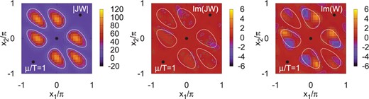
Absolute value of the statistical weight, |$|JW|$| (left), imaginary part of the statistical weight, |$\mathrm{Im}(JW)$| (middle), and imaginary part of the Boltzmann weight, |$\mathrm{Im}(W)$| (right), on the optimized path. We show the results at |$\mu/T=1$| on a |$30^2$| lattice. The optimized path is obtained in Method A. White curves show the contour of |$|JW|=20$|⁠.

In Fig. 2, we show |$y_1$|⁠, the imaginary part of |$z_1$|⁠, as a function of real parts, |$(x_1,x_2)$|⁠. The imaginary part of |$z_2$| is obtained by exchanging |$x_1$| and |$x_2$|⁠. We compare the results in Method A (left) and those in Method B (right). The standard gradient descent method and the feedforward neural network give qualitatively the same but somewhat different results of |$y_1$|⁠. In the statistically significant region (inside the white curve), these results are more consistent with each other. Since the cost function does not have sensitivity to the region with small weight, the results can be different outside of the statistically significant regions, as we expected.

Fig. 2.

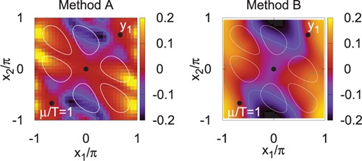
Imaginary part of |$z_1$| on the optimized path. We show |$y_1$|⁠, the imaginary part of |$z_1$|⁠, on the optimized path as a function of the real parts on a |$30^2$| lattice at |$\mu/T=1$| in Methods A (left) and B (right). White curves show the contour of |$|JW|=20$|⁠.

In Fig. 3, we show the average phase factor as a function of |$\mu/T$| obtained on the |$30^2$| and |$60^2$| mesh points in Method A. We show the difference from unity of the average phase factor. After optimization, the average phase factor is enhanced to be greater than |$0.997$|⁠, i.e., |$1-|{\langle{e^{i\theta}}\rangle_\mathrm{pq}}| < 3\times 10^{-3}$|⁠. While the average phase factor is large even without optimization, |$|{\langle{e^{i\theta}}\rangle_\mathrm{pq}}|>0.95$|⁠, the difference with and without optimization appears strongly in finite spatial volume cases, as discussed later. The minimum average phase factor appears at around |$\mu/T=0.5$|⁠.

Fig. 3.

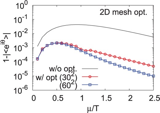
Average phase factor after path optimization on 2D mesh points in Method A. Results with mesh points of |$30^2$| (red circles) and |$60^2$| (blue squares) are shown in comparison with the average phase factor without optimization. We show the difference of the absolute values of the average phase factor from unity, |$1-|{\langle e^{i\theta} \rangle}|$|⁠.

As already mentioned, we clearly see that the statistical weight has six separate regions on the |$(x_1,x_2)$| plane in the diagonalized gauge. This separation comes from the structure of the Haar measure and it causes the numerical problem in Monte Carlo sampling: it is difficult to sample all of relevant regions beyond the energy barriers between them. It is, of course, not a problem in the mesh point integration, but we cannot apply the mesh point integration to more realistic problems in field theories because of its enormous numerical cost. Thus we proceed to discuss the results based on the Monte Carlo integral without diagonalized gauge fixing.

4.3. Results without diagonalized gauge fixing: Method C

Next, we discuss the results without diagonalized gauge fixing. Since we have eight independent variables, it is not possible to perform mesh point integration. We utilize the feedforward neural network to prepare and optimize the path, and we apply the hybrid Monte Carlo method to sample the configurations in Method C. Figure 4 shows the average phase factor with and without the path optimization. The path optimization is performed by using Method C and the results without the path optimization are estimated by using the 2D mesh point integration. We can clearly see that the path optimization increases the average phase factor in all values of |$\mu/T$| shown in the figure.

Fig. 4.

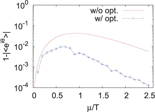
The average phase factor with (blue dots) and without (red line) optimization. Results with optimization are obtained by Method C. The expectation value without the optimization is obtained by using the 2D mesh point integral with diagonalized gauge fixing.

In Fig. 5, we show the expectation values of the chiral condensate (⁠|$\sigma$|⁠), the quark number density (⁠|$\rho$|⁠), and the Polyakov loop (⁠|$P$|⁠), as functions of |$\mu/T$| in comparison with exact results. Here, we use |$N_\mathrm{conf}=1000$| for |$\sigma$| and |$\rho$| and |$N_\mathrm{conf}=10\,000$| for |$P$|⁠. Since the fluctuation of |$P$| is larger than those of |$\sigma$| and |$\rho$|⁠, we need a larger number of configurations. The expectation values on the optimized integral path agree well with exact results within the error bar. The chiral condensate decreases rapidly in the |$\mu/T =0.5$|–|$1.0$| region and the Polyakov loop seems to stay at small values above |$\mu/T > 2$|⁠.

Fig. 5.

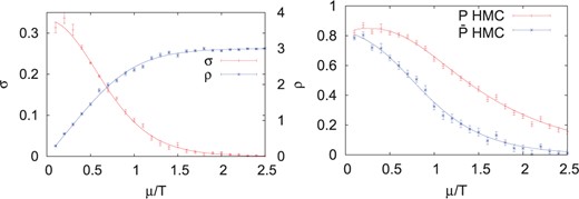
The expectation values of the quark condensate, the quark number density, and the Polyakov loop. The symbols show numerical results by using the hybrid Monte Carlo method, and the lines are analytic exact results.

It is interesting to check if we can reproduce the statistical weight distribution obtained in the diagonalized gauge (Methods A and B) shown in the left panel of Fig. 1 by using configurations obtained in Method C. We diagonalize the link variable by the similarity transformation, |$\mathcal{U}=P\mathcal{U}^{\mathrm{diag}}P^{-1}$|⁠, and |$(z_1,z_2)$| are specified by the diagonal matrix elements, |$\mathcal{U}^\mathrm{diag}=\mathrm{diag}(e^{iz_1},e^{iz_2},e^{iz_3})$|⁠. Figure 6 shows a scatter plot of the real part of |$z_1$| and |$z_2$|⁠. From the figure, we can see that the relevant six regions are actually visited in the Markov-chain hybrid Monte Carlo sampling.

Fig. 6.

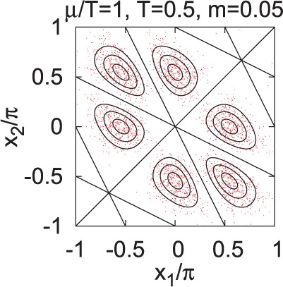
A scatter plot of |$(x_1,x_2)$| in Method C. The variables |$(x_1,x_2)$| are obtained by diagonalizing the link variables, specifying the eigenvalues as |$(e^{iz_1}, e^{iz_2}, e^{iz_3})$|⁠, and taking the real parts of |$(z_1,z_2)$|⁠. The configurations are generated by using the hybrid Monte Carlo method.

5. Summary

In this article, we have examined the validity and usefulness of the path optimization method in |$0+1$|D QCD. |$0+1$|D QCD is a toy model of the realistic |$3+1$|D QCD, but it contains the same terms, the temporal hopping terms of quarks, which causes the sign problem in |$3+1$| dimensions, so we can use it as a good laboratory to investigate several issues of the sign problem. It should be noted that there is a fake early onset problem of the baryon number (the Silver Blaze problem) in the phase reweighting method of |$3+1$|D lattice QCD. Since we cannot distinguish the quark number chemical potential and the isospin chemical potential in the phase-quenched weight, pions appear at |$\mu=m_\pi/2$| [48] and in addition the derivative of the partition function with respect to the quark chemical potential starts to grow at |$\mu=m_\pi/2$| rather than |$\mu=m_N/3$| [49]. Therefore further studies are needed in fermionic systems with such problems.

We have found that the path optimization method combined with the feedforward neural network is a useful tool to study the sign problem for several reasons. First, it can greatly improve the average phase factor. Second, the statistical weight distributions with and without diagonalized gauge fixing agree with each other. We find that, in |$0+1$|D QCD with diagonalized gauge fixing, the statistical weight distribution is separated into six regions, which could prevent us from sampling configurations equally well from these regions in Markov-chain Monte Carlo methods. However, the six regions are found to be well visited in Monte Carlo configurations generated without diagonalized gauge fixing. This fact indicates that the energy barriers in the variable space with the diagonalized gauge, |$(x_1,x_2)$|⁠, are apparent ones, and do not cause trouble in gauge-unfixed calculations. Thirdly, some of the observables are demonstrated to be obtained correctly. We have calculated the chiral condensate, the quark number density, the Polyakov loop, and its conjugate as functions of |$\mu/T$|⁠, and these results reproduce the exact ones within the errors. This is not surprising, since the integrals of holomorphic functions are independent of the path as long as the path does not go through singular points of the Boltzmann weight, which do not exist in the region of finite imaginary parts of integral variables.

The average phase factor without gauge fixing on the optimized path is found to be larger than 0.995. This value corresponds to the situation that the average phase factor is |$\sim 0.08$| on the |$8^3\times N_\tau$| lattice, provided that other terms in |$3+1$|D QCD do not make the average phase factor worse. The average phase factor of |$0.08$| seems to be small, but it is not impossible to perform Monte Carlo sampling with the current computer power. Compared with the 2D mesh point integration, the average phase factor is still smaller. Then it would be possible to further optimize the integral path by, e.g., modifying the cost function to be more sensitive to the average phase factor at around |${\langle{e^{i\theta}}\rangle_\mathrm{pq}} \simeq 1$|⁠. The path optimization method thus may be a promising method to overcome the sign problem in realistic QCD, if we can reduce the numerical cost and the upper limit of the average phase factor is sufficiently large. The numerical cost is dominated by the computation of the Jacobian, and a promising way to reduce this cost is the diagonal ansatz of the Jacobian matrix [35] and the nearest-neighbor lattice-site ansatz [36].

It should be noted that there exists an upper bound of the average phase factor less than unity in many fermionic models, and this upper bound may decrease exponentially as a function of spacetime volume. For example, the upper bound is found to be small in the Hubbard model [50,51] even with the Lefschetz thimble approach. From a mathematical viewpoint, the path optimization method belongs to the same class as the Lefschetz thimble approach, so similar upper bounds would also exist in the path optimization method. In principle, we cannot solve the “sign problem” with this kind of exponentially small upper bound in the path optimization method. However, approaching the upper bound allows us to enlarge the parameter region where we can calculate observables. For this purpose, it is desirable to develop a method to examine whether the average phase factor reaches the upper bound or not.

Acknowledgements

This work is supported in part by Grants-in-Aid for Scientific Research from Japan Society for the Promotion of Science (JSPS) (Nos. 15H03663, 16K05350, 18J21251, 18K03618, and 19H01898), and by the Yukawa International Program for Quark–Hadron Sciences (YIPQS).

Funding

Open Access funding: SCOAP|$^3$|⁠.