


Abstract
We explore the role of natural characteristics in determining the worldwide spatial distribution of economic activity, as proxied by lights at night, observed across 240,000 grid cells. A parsimonious set of 24 physical geography attributes explains 47% of worldwide variation and 35% of within-country variation in lights. We divide geographic characteristics into two groups, those primarily important for agriculture and those primarily important for trade, and confront a puzzle. In examining within-country variation in lights, among countries that developed early, agricultural variables incrementally explain over 6 times as much variation in lights as do trade variables, while among late developing countries the ratio is only about 1.5, even though the latter group is far more dependent on agriculture. Correspondingly, the marginal effects of agricultural variables as a group on lights are larger in absolute value, and those for trade smaller, for early developers than for late developers. We show that this apparent puzzle is explained by persistence and the differential timing of technological shocks in the two sets of countries. For early developers, structural transformation due to rising agricultural productivity began when transport costs were still high, so cities were localized in agricultural regions. When transport costs fell, these agglomerations persisted. In late-developing countries, transport costs fell before structural transformation. To exploit urban scale economies, manufacturing agglomerated in relatively few, often coastal, locations. Consistent with this explanation, countries that developed earlier are more spatially equal in their distribution of education and economic activity than late developers.
I. Introduction
The most obvious determinant of the spatial distribution of economic activity is geography: the degree to which locations are amenable to human habitation, output production, and the transport of goods. These geographical characteristics are frequently referred to as “first nature,” and their effects are well studied in the literature.1 But while the characteristics that constitute first nature are for the most part fixed over time, the effect that these characteristics have on the concentration of economic activity may alter in response to technological change (e.g., air conditioning and irrigation) as well as structural transformation (e.g., the Agricultural and Industrial Revolutions). Changes over time in the roles of geographic characteristics have not been well studied.
In this article, we take a systematic approach to analyzing changes in the effects on the density of economic activity of specific first-nature characteristics, focusing on what we believe to be the two areas in which the importance of such characteristics has changed the most. These are, first, the suitability of a region for growing food and, second, the suitability of a region for engaging in national and international trade. We establish several new and surprising facts. First, we show that the weight attached to the suitability of a region for growing food has declined over time, while the weight associated with suitability for trade has risen. Related to this first observation is a second: in developed countries, where agriculture represents a relatively small part of the economy, the location of overall economic activity is driven much more by factors determining agricultural productivity than trade suitability, compared to developing countries, where agriculture is a much larger component of GDP or the labor force. Many of us familiar with individual developed countries think of the strong role that location on lakes or rivers and access to the coast played in their historical evolution. However, we show explicitly that all the trade-related variables play a much more important role in today's developing countries. Finally, we find that countries that transformed and agglomerated into cities earlier also have greater spatial equality in the distribution of economic activity generally, and in educational attainment specifically, than those that agglomerated late.
Tying these observations together are two forces: technological change and persistence. Over the past several centuries (the period of time in which most of the agglomeration in the world has taken place), the link from ease of food production to concentration of economic activity has attenuated both because an increase in agricultural productivity has ensured that food represents a much smaller fraction of the consumption basket today than in the past, and because costs of transporting food have fallen dramatically. Thus, on both the production and consumption sides, there is less need for most of the population to live near where food is produced within a country. Similarly, suitability of a region for international trade via first-nature characteristics such as location on coasts, navigable rivers, or natural harbors, has become more valuable as opportunities to reap gains from trade have increased over the past 150 years.2 We show below that there were important differences in the relative timing of increased agricultural productivity and reductions in transport costs in early versus late developing countries.
Interacting with these changes in technology is persistence, which in turn results from urban agglomeration, the great force shaping the distribution of economic activity beyond first nature. It is precisely this persistence that also allows us to understand how the weights on geographic factors have changed over time, even though the highly detailed data on the spatial distribution of economic activity that we have access to does not have a usable time dimension. Specifically, although we can’t observe the detailed locations of historical agglomerations, we can sort countries by their degree of structural transformation and urbanization at a particular point in time and then rely on the fact that in those countries that agglomerated early, the current distribution of economic activity reflects the persistent effect of technology at the time of agglomeration. Several economic studies have examined such persistence in more localized settings (i.e., specific regions, or in response to particular shocks). Our article is the first to examine, and take advantage of, such persistence at a global scale.3
Our findings are relevant to current debates regarding regional development policy. Efforts by national governments and international advisors to encourage the growth of hinterland cities in developing countries seem to reflect in part an implicit reference to the experience of developed countries. For example, starting in 2005, Chinese planners set a vision for further expanding the highway network with intentions of “Developing the West” and “Revitalizing the Northeast.” Under the 12th five-year plan (2010–2015) this involved 66,000 km of national or provincial roads in the poorest regions, with even more planned in the 13th five-year plan.4 Similarly, for Sub-Saharan Africa, some economists within the World Bank view secondary city development as a key to economic growth and poverty reduction, and this view is reflected in strategic plans for several countries.5 To the extent that the spatial distribution of population in rich countries reflects the persistence of patterns established under old technology and institutions, rather than an efficient response to conditions prevalent today, such efforts are to some degree misplaced.
Although our primary interest is in studying the interaction of nature with history, we begin our empirical analysis by examining the overall predictive power of first-nature characteristics for the distribution of economic activity in modern cross-sectional data. Our primary dependent variable is light at night, as observed from satellites, aggregated to roughly 240,000 quarter degree (longitude/latitude) grid cells. Although, as discussed below, within-country variation in lights is primarily driven by variation in population density, we prefer the lights measure to available measures of population density from global population datasets (discussed in Section III), because lights data are sampled at uniformly high spatial resolution across countries (Henderson, Storeygard, and Weil 2012). We also consider as an outcome the spatial distribution of skills within countries (Gennaioli et al. 2013). Our measures of first nature include characteristics of the climate, land surface, natural water bodies, and plant life (temperature, precipitation, elevation and ruggedness, coasts, navigable rivers, natural ports, and biomes). We are particularly interested in the relative importance of characteristics related to suitability for trade (such as being located near a natural harbor, or the coast or on a navigable river or major lake) versus those associated with agricultural productivity.
A significant advance we make over much of the current literature is that we focus on the distribution of activity within countries. The most important reason for doing this is that economic density of a location, as well as our proxy for it, light density, is a function of both population density and income per capita. Focusing on within-country variation reduces the variance of income per capita, so that lights variation is driven primarily by the population distribution. In addition, institutions (for which countries are a convenient proxy) clearly matter for both income and population density. While geographic factors may well play a significant role in shaping institutions, sorting out the effect of institutions versus geography on the global distribution of economic activity in cross-country data is extremely difficult, if not impossible. By controlling for institutions and other national characteristics through country fixed effects, we are capturing direct first-nature effects on the distribution of resources within countries. The weights on geography that we estimate are thus not biased by any effect of geography on national level institutions or policies (such as trade policy). Our approach of including country fixed effects removes some geographic variation, but we show that a very large amount of usable variation remains.
The rest of this article is organized as follows. Section II presents some of the historical data that motivates our approach, outlines our conceptual framework, and describes a model which is fully specified in Online Appendix B. Section III describes our data on lights and physical geography. In Section IV we first discuss the interpretation of the lights data and then consider the explanatory power of geographic factors to predict global variation in observable lights, both overall and net of country fixed effects. Section V shows empirically the heterogeneity between early and late-developing countries, as well as a pattern of spatial inequality within countries consistent with our framework. Section VI concludes.
II. History and Conceptual Framework
The effect of physical geography on human settlement depends on the state of technology and the structure of the economy. When these change, the values attached to specific geographical characteristics change as well. There are numerous technological and economic changes whose effects one could trace over time. As discussed above, we think that the two that have been most important during the history of urbanization over the past few centuries are, first, the rise of labor productivity in agriculture, and second, the decline in transport costs and concomitant opening of possibilities for trade both within and between countries. In Section II.A we establish key facts about such changes, and in Section II.B we discuss a conceptual framework.
II.A. Historical Background
1. Urbanization and Food Production
Urbanization has been driven, above all, by rising labor productivity in agriculture, due in turn to both technological change and the substitution of other inputs for human power. Combined with low price and income elasticities of demand for food, this rise in labor productivity has produced an enormous drop in the fraction of workers found on farms. Prior to this transformation, population was necessarily diffuse, because of declining marginal product of labor when applied to a fixed quantity of land, and population density was tightly linked to the quality of agricultural land. Differences across countries in the timing of this change in agricultural productivity—for example, the British Agricultural Revolution starting in the seventeenth century and the Green Revolution in many developing countries after World War II—have been linked to corresponding differences in the timing of urbanization (Desmet and Henderson 2015).
Allen (2000) finds that output per worker in English agriculture increased 88% between 1600 and 1800. Correspondingly, the fraction of the labor force engaged in agriculture fell from 69% to 35% over the same period and the fraction living in cities rose from 10% to 29%.6 Although in later episodes of urbanization imports played a role in easing the food constraint, this was not the case in Europe in this period. According to Allen, in both the Netherlands and England, the two European regions most reliant on food imports, domestic production accounted for at least 90% of consumption through 1800. Similarly, in China, at a roughly similar date, long-distance trade in grain amounted to only 8% of national consumption (Shiue and Keller 2007).
Even in the modern world, food consumption in most countries is overwhelmingly supplied by domestic farming, and in developing countries, a large fraction of the labor force is required to produce that food, resulting in a low level of urbanization. Gollin, Parente, and Rogerson (2007) report that among developing countries in 2000, 55% of employment was in agriculture, with only a small part of that devoted to nonfood or export crops, while among the group of low-income countries, net food imports accounted for only around 5% of total calorie consumption. Looking at developing countries over the period 1960–2000, they show a very strong statistical relationship between increases in labor productivity in agriculture and declines in the agricultural share of the labor force, although this cannot necessarily be interpreted as a simple causal relationship. In the quantitative model they construct, differences in agricultural productivity growth are key in explaining the differential timing of takeoff across countries.
Bairoch (1988, Table 29.2) reports that among developed countries, the level of urbanization was 24% in 1880, a level that was not reached in the “third world” for another 85 years. Relatively consistent data begin in 1950 (United Nations 2014). In that year, urbanization rates were 56.6% in high-income countries, 19.8% in upper-middle income countries, 17.9% in lower-middle income countries, and 9.0% in low-income countries. By 2010, the rates for these groups were 79.3%, 58.8%, 37.7%, and 28.5%, respectively.7 Thus in the period after 1950, much of the developing world has been proceeding down a path of urbanization, often starting from a very low level, that the developed countries traversed at a much earlier point in time. Using a city cutoff size of 10,000, Jedwab and Moradi (2016) report that in a group of 39 Sub-Saharan African countries, the urbanization rate in 1960 was 1 percentage point higher than that observed in Europe in 1700 (9% versus 8%).
2. Persistence of Cities
The persistence of cities in terms of their locations and their relative sizes has been well studied, although there remains active debate about the relative importance of different causes, among them natural advantages, long-lived capital, location-specific knowledge accumulation, and history as an equilibrium-coordinating device. Bleakley and Lin (2012) show that U.S. cities whose locations were initially determined by particular geographical characteristics did not experience relative decline even when those geographical characteristics were no longer of value. They take this as evidence of path dependence. Jedwab, Kerby, and Moradi (2017) similarly show that locations of population agglomerations in Kenya and Ghana were persistent even after the factors that initially led to their establishment (such as colonial railroads and the presence of European settlers) disappeared. Davis and Weinstein (2002) find persistence of relative city sizes in Japan even after the shock of U.S. bombings in World War II, and similarly find persistence in regional densities in Japan over very long historical periods. Their preferred explanation puts heavy weight on persistent geographic advantages.
Eaton and Eckstein (1997) examine the 40 largest cities in France (1876–1990) and Japan (1925–1985) and find a very high degree of persistence in rank over the period of rapid industrialization and urbanization. Black and Henderson (2003) and Duranton (2007) similarly demonstrate the relative stability of the city size ordering and lack of downward mobility, in terms of population or employment, in the United States and France over the twentieth century.8
Finally, looking beyond city size rankings, a related point is that once a location begins to be urbanized, it usually stays that way. To see this, we consider the 119 European cities in 10 modern European countries in 1500, in the data set constructed by Wahl (2016). Despite five centuries of war, redrawing of borders, and massive structural change, only 15 of the 119 cities have fewer than 50,000 people today. We take this as evidence of persistence.9
3. Transport Costs
Transport costs have fallen over the past several centuries, most dramatically over the past 150 years, because of technological change, investments in infrastructure, and institutional changes such as reductions in internal and external tariffs and improvements in market institutions. The decline in trade costs had two effects that are relevant in our context. First, it further freed people from the necessity of living near where the food they eat is grown. Second, it raised the desirability of geographic characteristics that specifically facilitate trade, such as being on a coast or a navigable river.
Prior to the industrial revolution, bringing food from farms to cities was expensive almost everywhere in the world. In early modern Europe, Dittmar (2011) writes,
Transportation costs—especially for heavier products and overland transport—were exceedingly high. Grain transported 200 kilometers overland could see its price rise by nearly 100%. While the early modern period saw major developments in the international trade in grain, most cities remained heavily reliant on the provision of foodstuffs from within a circle of 20 to 30 kilometers which avoided heavy transport costs and the risks of reliance on foreign supplies.
Land-based goods, such as food and fuel, represented a large fraction of the consumption basket, and prices for these goods (such as bread) rose with city size, because of the need to transport them over greater distances.
Bairoch (1988) calculates that transporting grain by animal-drawn cart, even excluding indirect costs such as road maintenance, implied a doubling of prices at a distance of 260 kilometers. Shiue and Keller (2007) conclude that on the eve of the industrial revolution, shipping costs and the efficiency of institutions that supported trade in China and Western Europe were roughly comparable.10
Even as the industrial revolution picked up speed, transport could be very slow and expensive. To give an example, in 1817, freight transport from Cincinnati to New York City, via Ohio River keelboat to Pittsburgh, wagon to Philadelphia, and wagon plus river to New York, took 52 days. In 1816, turnpike transport cost 30 cents per ton-mile (in that year, the price of wheat in Cincinnati was |${\$}$|22.64 per ton).11 However starting later in the nineteenth century, transport costs fell dramatically. The ratio of transport costs to New York relative to farm-gate prices in Wisconsin and Iowa fell from roughly 80% in 1870 to 20% in 1910 (Williamson 1974). The price of ocean shipping fell by 0.88% per year in the first half of the nineteenth century and by 1.5% per year in the second half (Harley 1988). In the United States, real railroad freight costs per ton-mile fell by ⅔ between 1880 and 1940, and by the same factor between 1940 and 2000 (Redding and Turner 2015).
4. Relative Timing
In today's developed countries, structural transformation began well before the major declines in transport costs (Desmet and Henderson 2015). By contrast, among developing countries with low productivity agriculture, by 1950, and in many cases much earlier, transport costs had fallen with the building of colonial rails and roads as well as the use of trucks (Jedwab and Moradi 2016; Jedwab, Kerby, and Moradi 2017). Donaldson (forthcoming) explores the effect of the 67,247-km railroad network constructed in British India between 1853 and 1930, finding that it greatly reduced freight costs compared to existing road, river, and coastal transport networks, and similarly greatly reduced interregional price differentials for traded goods. Despite the presence of this transport network, however, India was only 17.0% urban in 1950 and 30.9% in 2010.12
This point can be made even more concrete by looking directly at transport costs in Africa, the world region in which such costs are highest, and urbanization lowest. Teravaninthorn and Raballand (2009) show that while internal transport costs in Africa today are indeed higher than in developed regions such as France and the United States, the difference is only in the range of a factor of 2 or 3. Given the enormous decline in transports costs in developed regions over the past 150 years, this means that transport costs in Africa are far lower than they were in developed countries during their periods of rapid agglomeration. In a similar vein, Limão and Venables (1999) compare the cost of shipping a standard 40-foot container from Baltimore to coastal versus landlocked countries in Africa. Shipping to a landlocked, low-income West African country is 64% more expensive than shipping to a coastal country of the same type, reflecting the well-known toll of bad roads and rails in Africa. But again, it is notable that the base used in this comparison (the cost of ocean shipping) is extremely low by historical standards. Even with their high additional costs, inland areas of Africa are connected to world markets at costs that are low by historical standards. Thus, urbanization is taking place in a relatively low transport cost environment in comparison to early developers.
II.B. Model
In the presence of geographical persistence, historical changes in the economic value of different natural characteristics can be inferred from the modern mapping from characteristics to density. In Online Appendix B, we develop a model showing how the relative timing of the two key historical changes we focus on—rising agricultural productivity and falling transport costs—can influence the spatial distribution of population.
In the model, a country has two regions, which we label coast and hinterland, and two sectors, food and manufacturing, where the latter occurs in cities and is subject to agglomeration economies and congestion. Demand for food is income and price inelastic. As in many new economic geography (NEG) models, labor is perfectly mobile, land is perfectly immobile, and interregional trade in manufactured goods is costly. And as in NEG models with scale economies, there are multiple equilibria in certain regions of parameter space. Technological improvements come in two forms: higher labor productivity in agriculture and lower costs for transporting goods. Consider a developed country today that experienced the agricultural revolution before much of the dramatic drop in transport costs. Higher agricultural productivity released farmers into manufacturing cities, but since transport costs were high, a city developed in each of its two regions, so farmers and cities could trade easily within each region. Later when transport costs fell and interregional trade was less costly, in key regions of parameter space where net urban scale effects are exhausted or net diseconomies have set in, interior and coastal cities both persist as stable equilibria. Hence, manufacturing cities are found in both coastal and hinterland regions, driven by initial endowments of agriculturally suitable land.
In contrast, consider a developing country today. Since transport costs fall before structural transformation, most labor remains in farming, leaving scale economies in any industrial city unexhausted. Lowered transport costs allow concentration of manufacturing production in one region, whether the region has a modest productivity advantage (i.e., by being on the coast) or not, to take advantage of urban scale, as manufactures can be cheaply traded across regions. Once structural transformation starts in these countries, the initial agglomeration persists and grows, with hinterland city development not emerging as an equilibrium (the equilibrium with just one city is “stable” with respect to population perturbations as long as its urban net diseconomies are not extreme).
In today's developed countries, cities are thus scattered across historically important agricultural areas; as a result, there is a relatively higher degree of spatial equality in the distribution of resources within these countries. By contrast, in today's developing countries, cities are concentrated more on the coast where transport conditions, compared to agricultural suitability, are more favorable. In practice (although this is not encompassed in our model), this has been enhanced by the decline in international transport and communication costs which have led to globalization and the enormous expansion in international trade. Developing countries have less urban activity in the hinterlands and a higher degree of spatial inequality in output. As these countries move further along the path of structural transformation, even greater proportions of population may agglomerate in coastal cities. Of course, to the extent that some developing countries such as India and China did have substantial numbers of interior cities in 1500, they show a greater role for agricultural factors and less for trade factors than other countries with fewer (or less persistent) major ancient cities. For example, Chandler (1987) records eight Chinese and six Indian interior cities with a population of more than 60,000 in 1500. In Sub-Saharan Africa, no cities crossed that threshold by 1500, and only four interior ones did by 1850.
While we highlight technological change in transportation and agriculture as the main drivers of change in the spatial distribution of economic activity, it is clear that several other forces have also been at work, often differentially affecting early and late agglomerators. Developing countries have on average spent a smaller share of their recent history as democracies, and that may induce urban concentration in one large city, typically the national capital where leaders can satisfy a key support base, especially in small countries (Ades and Glaeser 1995; Henderson and Wang 2007). Democratization introduces regional representation and demands from hinterland areas for a greater share of resources (Karayalcin and Ulubasoglu 2010). To the extent that mineral resource deposits are not restricted to highly accessible locations, they have the potential to induce dispersion. If exploiting these resources is labor intensive in poorer countries, this would encourage more interior towns. The urban sector itself has been subject to technological change increasing the importance of agglomeration in knowledge-intensive service sectors, for example, and decreasing the costs of congestion.
III. Data
In order to consider these ideas empirically, we need measures of economic activity and several components of physical geography, all available on a global scale. Our proxy for economic activity is night lights. Unlike Henderson, Storeygard, and Weil (2012) and most other quantitative work on lights, we use the radiance-calibrated version of the data (Elvidge et al. 1999; Ziskin et al. 2010). In normal operations, the light detection sensor is very good at detecting low levels of light in small cities. However, the strong amplification that enables this detection also saturates the sensor in the most brightly lit places, including the centers of most of the largest 100 cities in the United States, so that their values are top coded. The 2010 Global Radiance Calibrated Nighttime Lights data set we use combines the high amplification regime for low light places with a lower amplification regime for more brightly lit places. Thus, all topcoding is removed, with minimal loss of information about low light places. The lights data are distributed as a grid of pixels of dimension 0.5 arcminutes (|$\frac{1}{120}$| of a degree of longitude/latitude, or approximately 1 square kilometer at the Equator).13
We use lights as the measure of economic activity because it is measured consistently worldwide at the same spatial scale. Alternatively, we could have considered population. There are three main sources of global population data. Landscan14 and Worldpop (Stevens et al. 2015) use other geographic data to interpolate population within census geographic units, which has the potential to bias our estimates. The Gridded Population of the World (GPW; CIESIN and CIAT 2005) uses population data exclusively, assuming uniform population density within enumeration units larger than its native (2.5 arcminute) resolution. On average, this means that population estimates are more heavily smoothed in poorer countries with lower statistical capacity, as well as in more sparsely populated regions. This could also bias our results.
Of course, spatial variation in lights reflects not only variation in population density but also variation in income per capita. However, given a reasonable degree of population mobility within countries, light variation within countries will primarily reflect the spatial distribution of population. To make this point concrete, we conducted a simple exercise using data on log light density, log population density, and log GDP per capita for subnational regions, from Gennaioli et al. (2014). Without country fixed effects, the R2 of a regression of lights on population density alone on the right-hand side is 0.530. When income per capita is alone on the right-hand side the R2 is 0.285, and when both are included it is 0.778. By contrast, when the data are demeaned by country, the corresponding R2's are 0.775 for population density, 0.128 for income per capita, and 0.808 for both.15
Our other variables of interest are reported at several different geographic scales, ranging from |$\frac{1}{120}$| of a degree to |$\frac{1}{2}$| degree. For analysis, we convert them all to a grid of ¼-degree cells, with each cell covering approximately 770 square kilometers at the Equator, decreasing with the cosine of latitude.16 This scale is a compromise between the fine detail observed at the native resolution of several data sets and the computational practicality of coarser cells. It also allows us to be less concerned about spatial autocorrelation than we would be at finer scales, and to reduce true spillovers as well. At this resolution, our sample is 242,184 grid cells that fall on land.
To analyze the determinants of variation in economic activity across locations, we define three sets of explanatory variables, which we refer to as agricultural, trade, and base covariates. The base covariates are two variables that arguably affect both trade and agriculture. These are malaria and ruggedness. Malaria affects human ability to live in an area regardless of the economic activities they perform, and ruggedness, a measure of the local variance in elevation (Nunn and Puga 2012), increases the cost of both trade and agriculture.17 The index of the stability of malaria transmission, from Kiszewski et al. (2004), is based entirely on characteristics of local mosquito species and climate predictors of mosquito survival. It is thus exogenous to human settlement patterns.
Our agricultural covariates comprise six continuous variables (temperature, precipitation, length of growing period, land suitability for agriculture, elevation, and latitude) as well as a set of 14 biome indicators. The temperature variable is a long-run (1960–1990) average of UEA CRU, Jones, and Harris (2013) based on Mitchell and Jones (2005) and precipitation is the Willmott and Matsuura (2012) measure averaged over the same period. Length of growing period, in days, is from FAO/IIASA (2011). Land suitability is the predicted value of the propensity of a given parcel of land to be under cultivation based on four measures of climate and soil, from Ramankutty et al. (2002).18
Elevation, in meters, is from Isciences (2008). While high elevation locations often have poor transport, we believe that once distance to various types of water transport (see below) and ruggedness are controlled for, it is best interpreted as an agricultural variable. In practice, our main result is robust to redefining elevation as a “base” variable. We also control for the absolute value of latitude, which could affect agriculture even net of our climate controls.
Biomes are mutually exclusive regions encoding the dominant natural vegetation expected in an area, based on research by biologists. The distribution of 14 biomes is from Olson et al. (2001). We combine “tropical and subtropical dry broadleaf forests” with “tropical and subtropical coniferous forests” and combine “tropical and subtropical grasslands and savannas and shrublands” with “flooded grasslands and savannas” because each pair is broadly similar and because the second member of each pair contains less than 1% of cells globally. We exclude areas historically covered by permanent ice from analysis.
Our five trade variables focus on access to water transport. We calculate distances in kilometers from cell centroids to the nearest coast, navigable river, major lake, and natural harbor.19 Our specifications include indicators for the presence of each of these four features within 25 km of a cell centroid, as well as a continuous measure of distance to the coast.
Columns (1) and (2) of Table I report summary statistics for all of these variables.
Summary Statistics and Baseline Regression Results
| Summary statistics | Regression w/out FEs | Regression w/ FEs | ||||
|---|---|---|---|---|---|---|
| Mean (std. dev.) | Min, max | Coefficient | Shapley | Coefficient | Shapley | |
| (1) | (2) | (3) | (4) | (5) | (6) | |
| Dependent variable | ||||||
| ln(light/land pixels) | −3.357 | −5.684 | ||||
| (3.119) | 6.941 | |||||
| Base covariates | ||||||
| Ruggedness (OOOs) | 2.781 | 0 | −0.00764*** | 0.000505 | −0.0148*** | 0.000935 |
| (4.852) | 95.81 | (0.00196) | (0.00165) | |||
| Malaria index | 1.921 | 0 | −0.0340*** | 0.0181 | −0.0472*** | 0.0129 |
| (5.289) | 38.08 | (0.00248) | (0.00235) | |||
| Agriculture covariates | ||||||
| Tropical moist forest | 0.117 | 0 | −0.0126 | 0.165 | −0.207*** | 0.130 |
| (0.321) | 1 | (0.0750) | (0.0651) | |||
| Tropical dry forest | 0.0223 | 0 | 0.995*** | 0.244*** | ||
| (0.148) | 1 | (0.0942) | (0.0796) | |||
| Temperate broadleaf | 0.104 | 0 | 1.795*** | 1.304*** | ||
| (0.306) | 1 | (0.0701) | (0.0647) | |||
| Temperate conifer | 0.0330 | 0 | 0.776*** | 0.161** | ||
| (0.179) | 1 | (0.0815) | (0.0777) | |||
| Boreal forest | 0.166 | 0 | −0.483*** | −1.283*** | ||
| (0.372) | 1 | (0.0758) | (0.0808) | |||
| Tropical grassland | 0.121 | 0 | −0.803*** | −0.0349 | ||
| (0.326) | 1 | (0.0555) | (0.0479) | |||
| Temperate grassland | 0.0772 | 0 | 0.744*** | 0.938*** | ||
| (0.267) | 1 | (0.0649) | (0.0571) | |||
| Montane grassland | 0.0334 | 0 | 0.613*** | 0.719*** | ||
| (0.180) | 1 | (0.0798) | (0.0716) | |||
| Tundra | 0.122 | 0 | −0.846*** | −1.417*** | ||
| (0.327) | 1 | (0.0848) | (0.0885) | |||
| Mediterranean forest | 0.0242 | 0 | 0.843*** | 1.362*** | ||
| (0.154) | 1 | (0.0926) | (0.0885) | |||
| Mangroves | 0.00404 | 0 | 0.0228 | −0.443*** | ||
| (0.0634) | 1 | (0.160) | (0.138) | |||
| Desert | 0.175 | 0 | ||||
| (0.380) | 1 | |||||
| Temperature (deg. C) | 10.02 | −22.29 | 0.172*** | 0.0383 | 0.116*** | 0.0295 |
| (13.77) | 30.37 | (0.00335) | (0.00378) | |||
| Precipitation(mm/month) | 60.82 | 0.387 | −0.00897*** | 0.0112 | −0.0113*** | 0.0102 |
| (59.27) | 921.9 | (0.000404) | (0.000413) | |||
| Growing days | 139.6 | 0 | 0.00989*** | 0.0446 | 0.00851*** | 0.0364 |
| (99.04) | 366 | (0.000276) | (0.000275) | |||
| Land suitability | 0.275 | 0 | 2.692*** | 0.125 | 2.226*** | 0.102 |
| (0.320) | 1 | (0.0545) | (0.0521) | |||
| Abs(latitude) | 38.31 | 0.125 | 0.114*** | 0.0268 | 0.0338*** | 0.0144 |
| (20.93) | 74.88 | (0.00247) | (0.00328) | |||
| Elevation (km) | 0.605 | −0.187 | 0.521*** | 0.00640 | 0.0727*** | 0.00536 |
| (0.790) | 6.169 | (0.0239) | (0.0255) | |||
| Trade covariatesCoast | ||||||
| 0.0972 | 0 | 0.191*** | 0.00254 | 0.199*** | 0.00222 | |
| (0.296) | 1 | (0.0373) | (0.0300) | |||
| Distance to coast (000s km) | 0.486 | 0 | −0.685*** | 0.0102 | −0.656*** | 0.00770 |
| (0.481) | 2.274 | (0.0275) | (0.0318) | |||
| Harbor < 25 km | 0.0273 | 0 | 1.456*** | 0.0148 | 1.260*** | 0.0119 |
| (0.163) | 1 | (0.0652) | (0.0546) | |||
| River < 25 km | 0.0273 | 0 | 0.797*** | 0.00246 | 0.697*** | 0.00213 |
| (0.163) | 1 | (0.0623) | (0.0569) | |||
| Lake < 25 km | 0.0108 | 0 | 0.614*** | 0.000406 | 0.598*** | 0.000453 |
| (0.104) | 1 | (0.0867) | (0.0828) | |||
| Number of observations | 242,184 | 242,184 | 242,184 | |||
| R2 | 0.467 | 0.577 | ||||
Notes. The first two columns show means and standard deviations, and minima and maxima, for all geographic variables for the full sample. The third and fifth columns report OLS coefficient estimates from equation (1) on the full sample, with and without country fixed effects, respectively. Standard errors, clustered by 3 × 3 sets of grid squares, are in parentheses. *p < .1, **p < .05, ***p < .01. Columns (4) and (6) report the corresponding Shapley values for biomes as a group, and for all other right-hand-side variables individually. See text for variable definitions.
IV. Baseline Specification and Results
IV.A. Specification
Figure I shows the variation in (demeaned) lights worldwide. The lights data convey a great deal of information about the relative location of economic activity. More importantly for our purposes, lights map out the location of economic activity within countries. As noted above, lights reflect total economic activity, which is a combination of the number of people and the activity level per person. Lights are bright in northern India and the eastern United States, because while economic activity per person is lower in India, population density is higher.
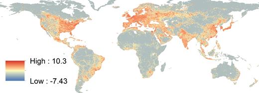
Demeaned ln(lights)
Full-color figure is available in the online version of this article.
We emphasize four further points about the lights data. First, some grid cells are partially covered by water or permanent ice. We thus divide the sum of lights on land by the number of constituent pixels (out of 900) that fall on land. Second, as noted already, cell area varies with latitude. However, since the raw lights values reflect density of emitted light (light emitted from a pixel divided by pixel area), no further adjustment is required. Third, light assigned to a particular pixel in the raw satellite data may partially reflect “overglow” of light emanating from nearby pixels (Small et al. 2005). This problem is greatly ameliorated by our collapsing of the data into grid cells composed of 900 pixels.
Finally and most importantly, almost 60% of our grid cells emit too little light for the satellite to detect. Since nearly all grid cells contain population and thus presumably emit some level of light, we consider this a censoring problem. The lowest nonzero values are generally interpreted as noise and recoded to zero at the pixel level in initial processing by NOAA.20 The lowest nonzero value of the sum of lights in a grid cell divided by the number of land pixels in the grid cell is 0.0034. We assign this value to grid cells with measured zeroes to avoid inducing excessive variation between them and the smallest nonzero values.21 Figure C1 in the Online Appendix plots the distribution of the dependent variable excluding the bottom code.
We emphasize three further points about equation (1). First, it is a very simple functional form. With such a large number of covariates, a second-order Taylor series has hundreds of terms, which improves the fit but limits interpretation.
Second, although we start by showing results both with and without country fixed effects, in the remainder of the article we show only fixed-effects results, since, as discussed above, our interest is in the determinants of within-country variation. Third, both the lights and the physical geography characteristics predicting them are highly spatially correlated. To the extent that this is manifested in spatially correlated errors, we have accounted for this by clustering errors within three-by-three squares of grid cells.22 However, spillover effects of measured explanatory variables are also possible. For example, an area with particularly fertile soil that attracts high population density also provides markets for neighboring areas with worse soils. We have tried to minimize the extent to which this affects our results by aggregating individual light pixels to much larger grid cells, which essentially internalizes agglomeration externalities. Thus, estimated coefficients are reduced form, reflecting endogenous agglomeration in addition to raw agricultural and trade effects.23
IV.B. Basic Results
Columns (3) and (5) of Table I report coefficients from a regression of our lights variable on the full suite of physical geography characteristics (equation (1)) without and with country fixed effects. The coefficients with and without fixed effects are generally of similar magnitudes and are of the same sign for all covariates. However, the high potential for collinearity limits inference from comparison of many individual coefficients. As an alternative, we plot fitted values from the two specifications in Panels A and B of Figure II, holding the color scale fixed, setting the country fixed effects to zero, and demeaning as in Figure I. The correlation of the fitted values is 0.861. This correlation, as well as a visual comparison of the two figures within continents and countries, suggest that the two specifications provide very similar predictions of which regions have high light density. In other words, the geographic forces that drive the allocation of economic activity within and across countries are similar. Of course, overall predictions of country lights relative to the mean differ somewhat between the two figures in some countries, because their fixed effects are correlated with some aspects of their geography. Thus, predicted values for countries in Africa overall look brighter relative to the mean in the fixed effects specification than in the non-fixed effects one because some of the coefficients of geographic variables have changed once African country fixed effects are accounted for. But importantly, the fixed effects change within-country patterns very little.
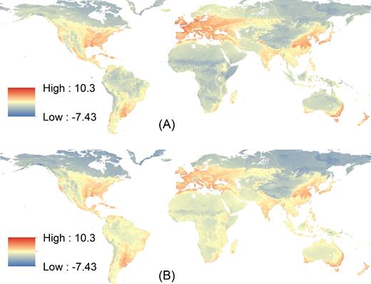
Panel A: Demeaned Predicted ln(lights) without Fixed Effects. Panel B: Demeaned Predicted ln(lights), Fixed Effects Specification with Fixed Effects Suppressed
Each map reports demeaned predicted values from a regression of ln(lights) on all geographic variables. In Panel B, the regression is run with country fixed effects, but predicted values are calculated setting those fixed effects to zero. Full-color figure is available in the online version of this article.
Coefficients on individual covariates in Table I, columns (3) and (5) are generally in the expected direction. The biomes with the largest fixed effects coefficients are temperate forests and grasslands along with Mediterranean forest. Most biomes have significantly more lights than deserts (the reference biome); tropical moist forest, boreal forests, tundra, and mangroves have significantly less in the fixed effects column. Being near the coast, lakes, navigable rivers and natural harbors is associated with more lights, as is a longer growing season and higher agricultural suitability. Net of growing season, land suitability, and biomes, higher temperatures and lower precipitation are associated with more lights, perhaps in part because of their residential consumer amenity value. In an alternative specification excluding growing season, land suitability, biomes, and country fixed effects (not shown), precipitation has a positive effect overall, as might be expected based on agricultural productivity. When entered in quadratic form (not shown), temperature increases lights at a decreasing rate while precipitation reduces lights also at a decreasing rate (of reduction). Net of ruggedness and coastal distance, higher elevation is associated with more lights.
Columns (4) and (6) report the results of a Shapley decomposition of the regressions with and without fixed effects, following Shorrocks (2013). Each row reports the average marginal contribution of the corresponding regressor to the overall R2 of the regression, across all permutations of the order in which variables are entered.24 Land suitability and the suite of biome measures contribute the most in the fixed effects specification, as well as fixed effects themselves, but growing days and temperature also contribute substantially. Individual trade variables add little on average.
Table II reports R2 and Shapley values by blocks of covariates: base variables (ruggedness and malaria), agricultural variables, trade variables, and country fixed effects. Shapley values and marginal R2 contributions are very high for agriculture and country fixed effects. While trade variables as a block have low Shapley values and marginal contribution to R2, we will see below that they are much more important in late agglomerator countries.
R2 and Shapley Values from Regressions Predicting ln(light/land pixels)
| No country FEs | With country FEs | |
|---|---|---|
| (1) | (2) | |
| Panel A: R2 | ||
| All variables (N = 242,184) | 0.467 | 0.577 |
| Base variables (malaria, ruggedness) | 0.020 | 0.355 |
| Agriculture variables (plus base) | 0.450 | 0.566 |
| Trade variables (plus base) | 0.066 | 0.370 |
| Country fixed effects | 0.345 | |
| Panel B: Shapley values | ||
| Base | 0.011 | 0.009 |
| Agriculture | 0.423 | 0.321 |
| Trade | 0.033 | 0.025 |
| Country FEs | 0.222 | |
Notes. Each entry in Panel A represents an R2 value from a separate regression of ln(light) on the right-hand-side variables listed in the row and column headings. Each column in Panel B corresponds to a separate regression. The values shown are Shapley values for the set of variables shown.
The first column shows that our 24 geographic variables account for 47% of the variation in lights globally. We consider it remarkable that such a parsimonious specification can account for so much of the variation in global economic activity, without explicit regard to agglomeration or history. Country-level variation adds relatively little once physical geography factors are accounted for. For example, although country fixed effects account for 35% of lights variation on their own, in column (5) of Table I, their marginal contribution beyond the geographic variables is just 11 percentage points. Conversely, the geographic factors add 23 percentage points in explaining variation on top of the fixed effects.
V. Heterogeneous Specification and Results
V.A. Preliminary Evidence
We start by considering how the residual variation from our baseline specification (Table I, column (5)) varies across countries in the context of the literature on the key role of one form of transport potential: coastal access (e.g., Rappaport and Sachs 2003). We define grid cells as coastal if their centroid is within 25 km of the ocean or an ocean-navigable river. For each country, we form the average residual for coastal grid cells and subtract the average residual for interior cells. In Figure III we then graph the relationship between each country's residual differential and average years of schooling in 1950, one measure we will later use to partition counties into early and late agglomerators; a similar picture holds for two alternative 1950 measures we will use, urbanization and GDP per capita. In Figure III this residual differential is high for low education countries, compared to high education countries. A regression of the residual differential on education yields a coefficient (std. err.) of −0.342 (0.065) and an R2 of 0.20. The figure tells us that low education counties have high coastal compared to interior residuals, meaning we have underassessed the role of coastal location for them by imposing common coefficients.
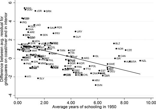
Difference between Average Coastal/River and Interior Residuals by Years of Schooling in 1950
ln(lights) are first regressed on all geographic variables in the global sample with country fixed effects, and residuals are calculated suppressing the fixed effects. These residuals are averaged separately within each country for two groups: cells within 25 km of a coast or navigable river and those farther away. The difference between these averages is the height of each point.
V.B. Heterogeneous Specification
To consider this pattern more formally, we partition the world into a set of early agglomerating countries and a set of late agglomerating countries. We define this partition primarily based on human capital, which allowed farmers to take advantage of higher-yield technologies. Panels A and B of Figure IV plot adult literacy rates over time for a variety of early and late agglomerators, respectively. The pattern is very clear. In panel A, many early agglomerators had literacy rates that were over 50% by the mid-nineteenth century, and in some cases much earlier. This indicates that human capital was relatively abundant before the precipitous decline in global freight costs in the late nineteenth and early twentieth century, also graphed. As discussed in Section II, freight costs declined rapidly until about 1920 and then leveled out before a further steep reduction after about 1970. In contrast, Panel B of Figure IV shows that literacy was quite low in several late agglomerators for which we have data well after the substantial decline in transport costs.25
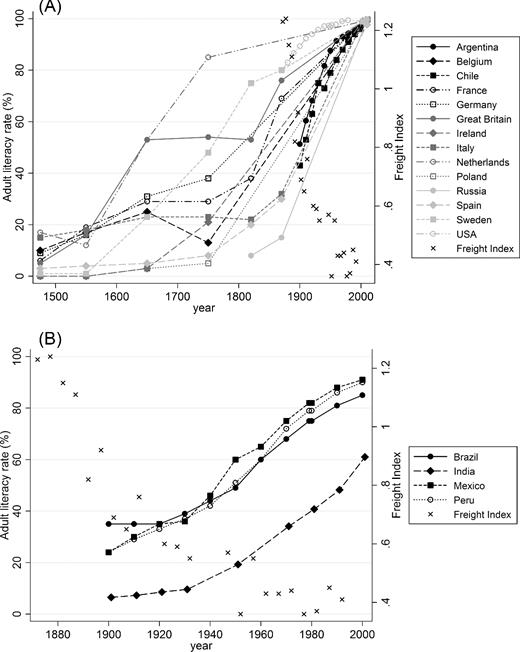
Panel A: Global Transport Costs and High Education Country Literacy Rates
Panel B: Global Transport Costs and Low Education Country Literacy Rates
The global real freight index is from Mohammed and Williamson (2004). Periods including world war years are omitted. Literacy rates for all countries except India are from Roser and Ortiz-Ospina (2016). Literacy rates for India are from UNESCO (1957), Ministry of Human Resource Development (1987), and World Bank (2015).
We operationalize our human capital measure using national average years of schooling in the adult population in 1950, the earliest year with comprehensive data, from Barro and Lee (2010). We consider two alternative measures indicating early agglomeration: GDP per capita (GDPpc) in 1950 from the Maddison Project (Bolt and van Zanden 2014), and more directly, the urbanization level in 1950 (United Nations 2014).26 The three measures are highly correlated, and results are similar for all. We focus on the education indicator in the text and figures because we think it is the most consistently measured, but results for all three are shown in the tables. Urbanization relies on definitions that vary substantially across countries, and the problems with cross-country comparisons of historical GDP are well known.
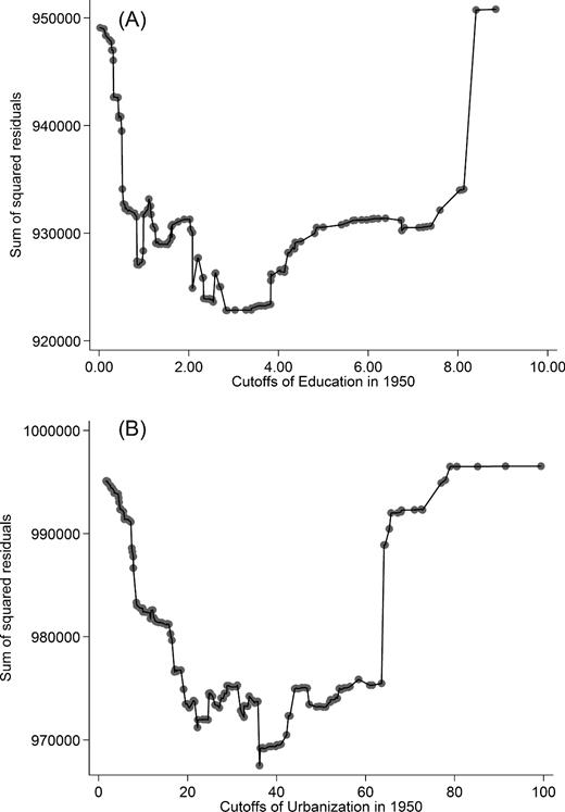
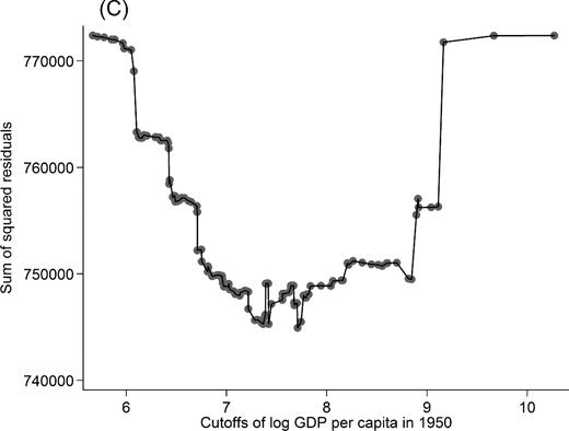
Panel A: Years of Schooling in 1950: Total SSR
Panel B: Urbanization in 1950: Total SSR
Panel C: GDP per Capita in 1950: Total SSR
In each panel, the vertical coordinate of each point represents the sum of squared residuals summed across two regressions on two disjoint samples, one each for countries above and below the cutoff of the cut variable specified on the horizontal axis. Each regresses ln(light) on all geographic variables and country fixed effects. Each point corresponds to an individual country in the sample (i.e., the exercise is run for each country's value of the cut variable and ranked by the cut variable).
V.C. Differential Results: Explanatory Power
Table III reports key results, the contribution of different blocks of variables in explaining lights variation within the early and late agglomeration samples, following equation (2). The top part of Panel A shows each variable set's contribution to R2 for low and high education countries. To highlight the comparison of interest, we can net out the contribution of the base variables. In the high education countries, the additional explanatory power of the agricultural variables is more than that of the trade variables. In the low education countries, it is the trade variables that offer relatively more explanatory power. Specifically, agriculture adds 0.27 to explanatory power relative to the base for high education countries but only 0.16 for low education. In contrast, trade adds 0.04 for high education countries compared to 0.10 for low education countries.
R2 Differentials of Trade and Agriculture Variables in Regression Predicting ln (light/Land pixels) for High/Low Education and Urbanization Countries
| Education | Urbanization | GDP per capita | ||||
|---|---|---|---|---|---|---|
| High | Low | High | Low | High | Low | |
| Countries | 58 | 82 | 63 | 121 | 36 | 101 |
| Observations | 126,671 | 100,361 | 138,020 | 103,975 | 80,310 | 100,602 |
| Panel A: R2 | ||||||
| Full sample | ||||||
| Base + FE | 0.385 | 0.294 | 0.351 | 0.362 | 0.387 | 0.375 |
| Agriculture + base + FE | 0.653 | 0.452 | 0.614 | 0.511 | 0.644 | 0.521 |
| Trade + base + FE | 0.425 | 0.395 | 0.386 | 0.452 | 0.419 | 0.467 |
| High - Low double differential | 0.171 | 0.170 | 0.171 | |||
| Panel B: Shapley values | ||||||
| Full sample | ||||||
| Base | 0.006 | 0.020 | 0.005 | 0.022 | 0.004 | 0.021 |
| Agriculture | 0.397 | 0.197 | 0.371 | 0.217 | 0.358 | 0.216 |
| Trade | 0.029 | 0.091 | 0.026 | 0.080 | 0.032 | 0.093 |
| Country FEs | 0.227 | 0.182 | 0.218 | 0.223 | 0.255 | 0.224 |
| Panel C: R2, hemispheres | ||||||
| New World | ||||||
| Base + FE | 0.245 | 0.236 | 0.253 | 0.258 | 0.239 | 0.264 |
| Agriculture + base + FE | 0.609 | 0.346 | 0.586 | 0.394 | 0.581 | 0.399 |
| Trade + base + FE | 0.303 | 0.321 | 0.297 | 0.343 | 0.286 | 0.348 |
| High - low double differential | 0.280 | 0.238 | 0.244 | |||
| Old World | ||||||
| Base + FE | 0.486 | 0.345 | 0.436 | 0.409 | 0.420 | 0.425 |
| Agriculture + base + FE | 0.706 | 0.528 | 0.661 | 0.569 | 0.611 | 0.580 |
| Trade + base + FE | 0.518 | 0.433 | 0.467 | 0.485 | 0.450 | 0.504 |
| High - low double differential | 0.092 | 0.111 | 0.085 | |||
Notes. Each number in the first three rows of Panel A is an R2 value from a separate regression of ln(light) on the set of right-hand-side variables listed in the row, for a sample defined by the column headings. The last row shows the double differential (Agriculture high − Trade high) − (Agriculture low − Trade low). FE stands for country fixed effects. Panel B shows the corresponding Shapley values, and Panel C is the analog of Panel A run separately for the Old and New Worlds. The cutoffs for education, urbanization, and GDP per capita are, respectively: 2.83 years of schooling, 36.16% urbanized, and |${\$}$|2,231 (2005 PPP).
The last row in Panel A summarizes this relationship, the relative advantage of agriculture over trade variables in explaining lights variation for high versus low education countries, in a double difference (e.g., (0.27–0.04) − (0.16–0.10)). Agriculture is relatively more important for early developing countries. The double differential is 0.17 for all three splits. Alternatively put, in early developing countries (by any of our three measures), agricultural variables incrementally explain at least six times as much variation in lights as do trade variables, while among late developing countries the ratio is roughly 1.5.
Panel B shows the relative contribution of agricultural versus trade variables as evidenced by Shapley values for high and low education countries. The Shapley value for agriculture variables is 14 times as large as that for trade variables in high education countries but only 2.1 times as large in low education countries. The pattern is similar for other sample splits, and consistent with the double-difference R2 results.
We note that this differential is not due to differences in absolute levels of variance in the geographic variables between the two samples. In other words, it is not simply the case that there is little within-country variation in the trade variables in early agglomerating countries, or little variation in the agriculture variables in late agglomerating countries. All five trade variables actually have a larger variance in the early agglomerators. Eight of 17 agricultural variables have a larger variance in the late agglomerators. Even among those agricultural variables with a larger variance in the early agglomerators, the differentials in standard deviations, except for a few biomes, are within 50% of the global standard deviation.
Finally, we consider the possibility that the relevant distinction is not between early and late agglomerators as we have conceptualized them, but rather between the Old World and the New World, where European conquest reset settlement patterns. Of course, equation (2) will have more explanatory power than equation (1) regardless of the split variable used, and a New–Old World split yields similar explanatory power as the high-low education, urbanization, or GDPpc splits. However, Panel C of Table III shows these other splitting variables are not simply proxies for the New World–Old World split. The relative advantage of agriculture over trade variables in explaining lights variation for high versus low education countries (or high versus low urbanization or GDPpc countries) is present in both New and Old World countries. In other words, results are consistent with our model within the New World and within the Old World. We do note that the double differentials are greater in the New World, where the influence of pre–Industrial Revolution interior and often ancient cities in the developing world may be less. That is, we start our experiment with a cleaner slate.
V.D. Differential Results: Marginal Effects
Table III emphasized the overall explanatory power of groups of trade and agricultural variables in the two samples. We now consider the differential in their relative marginal effects. If marginal effects of trade variables, relative to marginal effects of agricultural variables, are stronger in late agglomerator countries than in early agglomerator countries, this is consistent with the explanatory power results. Table IV reports estimated coefficients from equation (2). Column (1) shows the main effect, which is for low education countries, and column (2) shows the differential for high education ones, with analogous results for the other split variables in columns (3)–(6). In general, interaction effects are significant. We focus on the differential in the trade variables. The main effects show that for late agglomerators (developing countries), being near a coast, lake, navigable river, and natural harbor are all associated with increased intensity of economic activity, as is proximity to the coast entered as linear distance. However, the interaction effects are all offsetting, meaning that effects are all weaker in early agglomerating, high-income countries. Three of the variables have a net effect indistinguishable from zero for early agglomerators. River location retains a positive but greatly diminished effect. Only natural harbor presence has a strong (albeit still relatively diminished) effect for early agglomerators. The strength of these trade variable results may seem surprising, but they are exactly what our framework predicts. For agricultural variables the pattern is less distinct. We expect but do not always see heightened effects for high education countries. The relative effects of land suitability and growing days may be masked by the biome variables, some of which are distributed quite unevenly between the two groups of countries.
Regression Results Allowing Interactions between Geographic Variables and Early Agglomerator Dummy
| Education | Urbanization | GDP per capita | ||||
|---|---|---|---|---|---|---|
| Main effect | Interaction | Main effect | Interaction | Main effect | Interaction | |
| (1) | (2) | (3) | (4) | (5) | (6) | |
| Base covariates | ||||||
| Ruggedness (OOOs) | −0.0169*** | 0.00995*** | −0.0189*** | 0.00550* | −0.0154*** | 0.0166*** |
| (0.00283) | (0.00361) | (0.00255) | (0.00334) | (0.00258) | (0.00388) | |
| Malaria index | −0.0267*** | −0.0634*** | −0.0252*** | −0.124*** | −0.0247*** | −0.122*** |
| (0.00273) | (0.00863) | (0.00245) | (0.00984) | (0.00251) | (0.00936) | |
| Agriculture covariates | ||||||
| Tropical moist forest | −0.0667 | 0.812*** | 0.259*** | −1.992*** | 0.290*** | −2.164*** |
| (0.0802) | (0.239) | (0.0759) | (0.193) | (0.0759) | (0.188) | |
| Tropical dry forest | 0.376*** | 0.363 | 0.501*** | −0.540*** | 0.550*** | −0.722*** |
| (0.0912) | (0.336) | (0.0910) | (0.190) | (0.0907) | (0.191) | |
| Temperate broadleaf | 0.982*** | 0.259* | 1.035*** | 0.373*** | 0.994*** | 0.145 |
| (0.0912) | (0.137) | (0.0870) | (0.128) | (0.0876) | (0.143) | |
| Temperate conifer | 0.322*** | −0.170 | 0.573*** | −0.419*** | 0.434*** | −0.434** |
| (0.120) | (0.164) | (0.116) | (0.156) | (0.115) | (0.171) | |
| Boreal forest | −0.0237 | −1.041*** | −0.0352 | −0.882*** | −0.223 | −1.741*** |
| (0.133) | (0.172) | (0.136) | (0.169) | (0.138) | (0.193) | |
| Tropical grassland | −0.0181 | −0.360*** | 0.154*** | −0.428*** | 0.170*** | −0.688*** |
| (0.0659) | (0.107) | (0.0587) | (0.101) | (0.0589) | (0.105) | |
| Temperate grassland | 0.440*** | 0.375*** | 0.370*** | 0.622*** | 0.0608 | 0.771*** |
| (0.0880) | (0.126) | (0.101) | (0.126) | (0.111) | (0.147) | |
| Montane grassland | 0.306*** | 1.154*** | 0.462*** | 0.947*** | 0.480*** | 0.748*** |
| (0.0988) | (0.166) | (0.0921) | (0.152) | (0.0928) | (0.168) | |
| Tundra | −0.717*** | −0.634*** | −1.585*** | |||
| (0.116) | (0.107) | (0.148) | ||||
| Mediterranean forest | 1.999*** | −1.189*** | 1.951*** | −1.083*** | 1.840*** | −1.100*** |
| (0.130) | (0.166) | (0.130) | (0.165) | (0.124) | (0.165) | |
| Mangroves | −0.945*** | 0.765* | −0.378** | −1.116*** | −0.442*** | −0.909** |
| (0.165) | (0.443) | (0.164) | (0.323) | (0.163) | (0.390) | |
| Temperature (deg. C) | 0.121*** | −0.0238*** | 0.133*** | −0.0397*** | 0.122*** | −0.148*** |
| (0.00790) | (0.00903) | (0.00768) | (0.00881) | (0.00774) | (0.0112) | |
| Precipitation (mm/month) | −0.0101*** | 0.00176** | −0.00943*** | 0.000307 | −0.0103*** | 0.0000965 |
| (0.000563) | (0.000780) | (0.000542) | (0.000745) | (0.000567) | (0.000816) | |
| Growing days | 0.00711*** | 0.00129** | 0.00716*** | 0.00125** | 0.00733*** | 0.00166*** |
| (0.000398) | (0.000551) | (0.000372) | (0.000527) | (0.000377) | (0.000569) | |
| Land suitability | 2.158*** | −0.0960 | 2.070*** | 0.0743 | 1.981*** | −0.139 |
| (0.0774) | (0.110) | (0.0746) | (0.104) | (0.0755) | (0.118) | |
| Abs (latitude) | 0.0886*** | −0.0921*** | 0.102*** | −0.110*** | 0.1000*** | −0.189*** |
| (0.00564) | (0.00685) | (0.00540) | (0.00661) | (0.00542) | (0.00790) | |
| Elevation (km) | 0.248*** | −0.635*** | 0.222*** | −0.363*** | 0.167*** | −0.711*** |
| (0.0408) | (0.0576) | (0.0392) | (0.0543) | (0.0395) | (0.0593) | |
| Trade covariates | ||||||
| Coast | 0.915*** | −0.995*** | 0.706*** | −0.669*** | 0.735*** | −0.559*** |
| (0.0701) | (0.0767) | (0.0640) | (0.0712) | (0.0624) | (0.0747) | |
| Distance to coast (OOOs km) | −1.430*** | 1.540*** | −1.460*** | 1.389*** | −1.512*** | 1.367*** |
| (0.0472) | (0.0647) | (0.0469) | (0.0632) | (0.0471) | (0.0956) | |
| Harbor < 25 km | 1.564*** | −0.345*** | 1.365*** | −0.129 | 1.216*** | 0.0546 |
| (0.104) | (0.123) | (0.0949) | (0.115) | (0.0871) | (0.115) | |
| River < 25 km | 1.208*** | −0.772*** | 0.914*** | −0.359*** | 0.944*** | −0.520*** |
| (0.104) | (0.120) | (0.105) | (0.120) | (0.106) | (0.130) | |
| Lake < 25 km | 0.762*** | −0.346** | 0.548*** | 0.0182 | 0.730*** | −0.310* |
| (0.133) | (0.170) | (0.149) | (0.177) | (0.137) | (0.170) | |
| N | 227,032 | 241,995 | 180,912 | |||
Notes. Each set of two consecutive columns reports OLS coefficient estimates from a separate regression of equation (2) on a global sample, split by education, urbanization, and GDP per capita, respectively, in 1950. The first column in each pair shows main terms, and the second column shows interaction terms. Standard errors, clustered by 3 × 3 sets of grid squares, are in parentheses. *p < .1, **p < .05, ***p < .01.
Differential Coefficient Results
| Education | Urbanization | GDP per capita | |
|---|---|---|---|
| Agriculture differential (α) | 0.332*** (0.0238) | 0.193*** (0.0209) | 0.254*** (0.0239) |
| Trade differential (γ) | −0.650*** (0.0178) | −0.393*** (0.0218) | −0.526*** (0.0321) |
| N | 227,032 | 241,995 | 180,912 |
| Education | Urbanization | GDP per capita | |
|---|---|---|---|
| Agriculture differential (α) | 0.332*** (0.0238) | 0.193*** (0.0209) | 0.254*** (0.0239) |
| Trade differential (γ) | −0.650*** (0.0178) | −0.393*** (0.0218) | −0.526*** (0.0321) |
| N | 227,032 | 241,995 | 180,912 |
Notes. Each column reports nonlinear least squares estimates of α and γ in equation (3), for education, urbanization, and GDPpc split variables. Standard errors, clustered by 3 × 3 sets of grid squares, are in parentheses. *p < .1, **p < .05, ***p < .01.
As a means of visualizing how the determinants of agglomeration location have changed over time, we examine the difference between fitted values generated using the estimates for early developing countries and those generated using estimates for late developers. We can generate both sets of these fitted values for every country, regardless of whether it actually developed early or late. The larger the difference between these two estimates, the more that grid cell is favored by the coefficients that governed early developers relative to those that govern late developers. In practice, this is equivalent to constructing fitted values of |$( {\alpha X_{ic}^A{\beta _A} + \gamma X_{ic}^T{\beta _T}} )$| in equation (3). Figure VI shows this difference in fitted values for Europe, Africa, and parts of western Asia, using the education split.
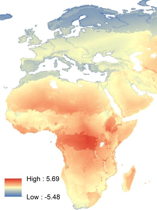
Demeaned Difference between High and Low Predicted Lights with Fixed Effects Suppressed
This map shows fitted values of |$( {\alpha X_{ic}^A{\beta _A} + \gamma X_{ic}^T{\beta _T}} )\ $|from equation (3). Color figure available in online version of this article.
In Africa, for example, interior areas such as the Congo basin and the Ethiopian highlands would have had higher light density under the early development regime than under the late development regime (which is in fact what applied to them). Similarly, in Africa, the areas around navigable rivers, particularly the Nile and Niger, have higher predicted densities under late development than if the region had developed early. Within Europe, coastal areas, which of course already have particularly high density, would have had even higher density if Europe had developed late instead of early. It is also interesting to note that Europe has predominantly negative values for the difference between predicted lights using early developer coefficients and predicted lights using late developer coefficients. This means that Europe is particularly rich in characteristics that favor population density in late developers, despite the fact that it developed early.
V.E. Spatial Inequality
Our conceptual framework provides a further prediction concerning spatial inequality. Early agglomerators, with their hinterland activity focused around agriculturally suitable land, should have a higher degree of spatial equality in lights overall than late agglomerators, where activity is concentrated near discrete, trade-friendly features (coasts, natural harbors, etc.). To test this prediction, we calculate a spatial Gini coefficient across cells for each country. Analogously to a typical Gini, we first construct a Lorenz curve by plotting the cumulative distribution of lights against the cumulative distribution of cells. The Gini is then the area between the 45-degree line and the Lorenz curve divided by the total area under the 45-degree line.
Figure VII plots this Gini for each country against 1950 schooling. As predicted, the Gini falls as education rises, with many African countries in the upper left corner having very high Gini values. However, there is enormous heterogeneity. Countries like Canada, the United States, and Australia with huge tracts of essentially uninhabitable land also have high Ginis. We thus regress the Gini on 1950 education (and urbanization and GDPpc) now in continuous form given the use of country-level data, and add key controls. Table VI reports results, and as usual we focus on the education results in columns (1)–(3), as the urbanization and GDPpc results are very similar. Column (1) reports the regression equivalent of Figure VII. A one standard deviation increase in schooling (2.35 years) is associated with a 0.06 reduction (0.40 standard deviations) in the Gini. Column (2) adds a control for the Gini of predicted lights based on the Table I fixed effects specification. This is the inequality that we would expect from geography alone. That heightens the negative marginal effect of education. Column (3) then adds in controls for log country land area and log population, which greatly increases the R2 as expected and returns the marginal effect very close to its value in column (1).
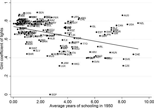
Gini Coefficient of Lights by Years of Schooling in 1950
Gini Coefficient of Lights
| (1) | (2) | (3) | (4) | (5) | (6) | (7) | (8) | (9) | |
|---|---|---|---|---|---|---|---|---|---|
| Education 1950 | −0.0265*** (0.00569) | −0.0325*** (0.00554) | −0.0263*** (0.00445) | ||||||
| Urbanization 1950 | −0.00283*** (0.000768) | −0.00303*** (0.000648) | −0.00179*** (0.000495) | ||||||
| ln(GDP per cap. 1950) | −0.0304** | −0.0418** | −0.0267 | ||||||
| (0.0145) | (0.0189) | (0.0167) | |||||||
| Gini of predicted lights | 0.249*** | 0.0809 | 0.315*** | 0.0503 | 0.189* | 0.0284 | |||
| (0.0801) | (0.0525) | (0.0753) | (0.0556) | (0.0995) | (0.0689) | ||||
| ln(land area) | 0.0675*** | 0.0704*** | 0.0714*** | ||||||
| (0.00698) | (0.00579) | (0.00690) | |||||||
| ln(population in 2010) | −0.0486*** | −0.0343*** | −0.0512*** | ||||||
| (0.00783) | (0.00675) | (0.00880) | |||||||
| Constant | 0.741*** | 0.648*** | 0.344*** | 0.734*** | 0.609*** | 0.167*** | 0.895*** | 0.896*** | 0.479*** |
| (0.0163) | (0.0391) | (0.0672) | (0.0212) | (0.0331) | (0.0586) | (0.101) | (0.112) | (0.126) | |
| N | 140 | 140 | 139 | 184 | 184 | 181 | 137 | 137 | 135 |
| R2 | 0.157 | 0.242 | 0.600 | 0.126 | 0.241 | 0.583 | 0.033 | 0.077 | 0.511 |
Notes. Each column reports OLS coefficient estimates from a country-level regression of the Gini coefficient of lights on the variables shown.
Robust standard errors are in parentheses. *p < .1, **p < .05, ***p < .01.
Table VI and Figure VII show that there is a strong association between the degree of early agglomeration and spatial equality. We have interpreted this through the lens of persistence and early versus late agglomerators. A reading of Williamson (1965) might suggest a complementary explanation in a spatial version of the Kuznets curve. Many late agglomerators are in the midst of structural transformation. During that transition, as countries urbanize we expect spatial inequality to rise as transforming regions where urbanization is focused have increased incomes per capita relative to the rural regions from which they are drawing people out of agriculture. As development proceeds, eventually incomes per capita will tend to converge across initially disparate regions as shown in Barro and Sala-i-Martin (1995, chapter 11) for some of our early agglomerators. Thus, part of the enhanced inequality of late agglomerators in Figure VII may arise from this ongoing transition. Our focus is on population allocation as reflected by lights, and our story is more about the inequality in agglomeration across regions than differences in income per capita. However, the two are related as we see next.
This association between spatial inequality in economic activity and likelihood of early agglomeration extends to spatial inequality in educational achievement. Table VII and Figure VIII show the degree of within-country spatial inequality in educational achievement using data from Gennaioli et al. (2013). These authors report average years of schooling for administrative regions at the first subnational level of governance (e.g., state/province) in 107 countries. Figure VIII plots a population-weighted Gini of this contemporary schooling measure against 1950 average schooling for each country. Again, we see the downward slope, indicating inequality declining as schooling and likelihood of early agglomeration rise. Table VII shows the analogous regressions for education, urbanization, and GDPpc in 1950, with and without controls for country land area and population. The slope of the 1950 variables are consistently negative in all specifications.
Education Ginis
| (1) | (2) | (3) | (4) | (5) | (6) | |
|---|---|---|---|---|---|---|
| Years of schooling in 1950 | −0.0183*** (0.00276) | −0.0193*** (0.00285) | ||||
| Urbanization in 1950 | −0.00224*** (0.000362) | −0.00228*** (0.000368) | ||||
| Log GDP per capita in 1950 | −0.0532*** (0.00939) | −0.0576*** (0.0103) | ||||
| Log area (sq km) | 0.00656 (0.00533) | 0.0119** (0.00562) | 0.0152** (0.00698) | |||
| Log population in 2010 | −0.0131** (0.00575) | −0.0101* (0.00597) | −0.0207** (0.00819) | |||
| Constant | 0.149*** (0.0149) | 0.198*** (0.0474) | 0.163*** (0.0175) | 0.115** (0.0451) | 0.496*** (0.0761) | 0.542*** (0.103) |
| Observations | 97 | 97 | 106 | 106 | 88 | 88 |
| R2 | 0.322 | 0.354 | 0.305 | 0.330 | 0.278 | 0.336 |
Notes. Each column reports OLS coefficient estimates from a country-level regression of the Gini coefficient of years of schooling on the variables shown. Robust standard errors are in parentheses. *p < .1, ** p < .05, ***p < .01.
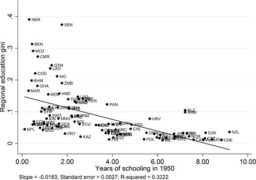
Population-Weighted Regional Education Gini by Years of Schooling in 1950
Again, part of this differential in inequality could follow the spatial transition and convergence story in Williamson and Barro and Sala-i-Martin. But it also relates to the recent urban literature on sorting across space (Behrens, Duranton, and Robert-Nicoud 2014). Large agglomerations attract relatively more high-skilled workers first because they specialize in skill-intensive business and financial services (Davis and Dingel 2014), and second because they facilitate learning more effectively for these high-skilled workers (Puga and de la Roca 2017). In the context of our story, that suggests that in late agglomerators, hinterland regions have a strong disadvantage in attracting high-skill workers away from large cities on the coast.
VI. Conclusion
In this article we have explored the role of natural characteristics in determining the location of economic activity, with a focus on the within-country distribution. Natural characteristics have a surprisingly high degree of overall explanatory power, but when we divide these natural characteristics into those associated with agricultural productivity and those associated with ease of trade, a puzzle emerges. In early developing countries, agricultural variables incrementally explain at least six times as much variation in lights as do trade variables, while among late developing countries the ratio is roughly 1.5. Correspondingly, the marginal effects of agricultural variables as a group on lights are 19–33% larger in absolute value for countries that developed early compared to those that developed later, while the marginal effects of trade variables are 39–65% smaller. The puzzle is that early developing countries, where agricultural variables are more important in explaining the location of economic activity, tend to be wealthy and have much smaller agricultural sectors than countries that developed later.
We see the resolution of this puzzle in the intersection of three forces. The first is persistence, the strong tendency for spatial patterns of agglomeration, once established, to remain in place. The second is the changing weights on different natural characteristics as economies develop. The two most important changes, in our view, are a reduction in the weight of characteristics associated with agricultural productivity and an increase in the weight of characteristics associated with trade. Finally, the third force is that early and late developing countries experienced changes in the weights associated with sets of natural characteristics in a different order.
In today's developed countries, the process of agglomeration and structural transformation began early, when transport costs were still relatively high, so urban agglomerations arose in multiple agricultural regions. High costs of trade protected local markets. In later developing countries, transport costs fell well before structural transformation started. To exploit urban scale economies with a limited national urban labor force, manufacturing tended to agglomerate in relatively few, often coastal, locations. With structural transformation, these initial coastal locations grew, while cities formed more rarely in the agricultural interior. Another implication of these forces is that spatial inequality in the distribution of resources within countries will be greater in today's developing countries compared to countries that developed earlier. Agricultural fundamentals drove the location of economic activity in developed countries, while cost of trade fundamentals play a much bigger role in developing countries.
Thus, the article tells us that we shouldn’t expect spatial development in poor and middle-income countries to follow the same pattern observed in countries that urbanized earlier. This observation has potential policy implications. The drive to invest in infrastructure to develop hinterland cities in China and parts of Sub-Saharan Africa, perhaps with implicit reference to the experience of developed countries, may be somewhat misguided, given the new weights on geographic fundamentals for these areas.
APPENDIX
Summary Statistics for National Variables
| Variable | N | Mean | Std. dev. | Min | Max |
|---|---|---|---|---|---|
| Years of schooling in 1950 | 140 | 2.92 | 2.35 | 0.02 | 9.19 |
| Urbanization in 1950 | 184 | 30.68 | 22.81 | 1.70 | 100.00 |
| GDP per capita in 1950 | 137 | 2,476.71 | 4,028.84 | 289.15 | 30,387.13 |
| Variable | N | Mean | Std. dev. | Min | Max |
|---|---|---|---|---|---|
| Years of schooling in 1950 | 140 | 2.92 | 2.35 | 0.02 | 9.19 |
| Urbanization in 1950 | 184 | 30.68 | 22.81 | 1.70 | 100.00 |
| GDP per capita in 1950 | 137 | 2,476.71 | 4,028.84 | 289.15 | 30,387.13 |
1950 Values by Country
| GDP | High | High | High | |||
|---|---|---|---|---|---|---|
| Country | Education | Urbanization | per cap. | educ. | urban. | GDPpc |
| Afghanistan | 0.3 | 5.8 | 645 | 0 | 0 | 0 |
| Albania | 2.6 | 20.5 | 1,001 | 0 | 0 | 0 |
| Algeria | 0.8 | 22.2 | 1,365 | 0 | 0 | 0 |
| Andorra | 38.8 | 1 | ||||
| Angola | 7.6 | 1,052 | 0 | 0 | ||
| Argentina | 4.8 | 65.3 | 4,987 | 1 | 1 | 1 |
| Armenia | 7.2 | 40.3 | 1 | 1 | ||
| Australia | 8.0 | 77.0 | 7,412 | 1 | 1 | 1 |
| Austria | 6.0 | 63.6 | 3,706 | 1 | 1 | 1 |
| Azerbaijan | 45.7 | 1 | ||||
| Bahamas | 52.1 | 1 | ||||
| Bahrain | 1.0 | 64.4 | 2,104 | 0 | 1 | 0 |
| Bangladesh | 0.9 | 4.3 | 540 | 0 | 0 | 0 |
| Belarus | 26.2 | 0 | ||||
| Belgium | 6.8 | 91.5 | 5,462 | 1 | 1 | 1 |
| Belize | 7.2 | 55.3 | 1 | 1 | ||
| Benin | 0.4 | 5.0 | 1,084 | 0 | 0 | 0 |
| Bhutan | 2.1 | 0 | ||||
| Bolivia (Plurinational State of) | 2.3 | 33.8 | 1,919 | 0 | 0 | 0 |
| Bosnia and Herzegovina | 13.7 | 0 | ||||
| Botswana | 1.4 | 2.7 | 349 | 0 | 0 | 0 |
| Brazil | 2.1 | 36.2 | 1,672 | 0 | 0 | 0 |
| Brunei Darussalam | 2.0 | 26.8 | 0 | 0 | ||
| Bulgaria | 3.8 | 27.6 | 1,651 | 1 | 0 | 0 |
| Burkina Faso | 3.8 | 474 | 0 | 0 | ||
| Burundi | 0.4 | 1.7 | 360 | 0 | 0 | 0 |
| Cabo Verde | 14.2 | 450 | 0 | 0 | ||
| Cambodia | 0.4 | 10.2 | 482 | 0 | 0 | 0 |
| Cameroon | 0.7 | 9.3 | 671 | 0 | 0 | 0 |
| Canada | 7.6 | 60.9 | 7,291 | 1 | 1 | 1 |
| Central African Republic | 0.4 | 14.4 | 772 | 0 | 0 | 0 |
| Chad | 4.5 | 476 | 0 | 0 | ||
| Chile | 4.8 | 58.4 | 3,670 | 1 | 1 | 1 |
| China | 1.6 | 11.8 | 448 | 0 | 0 | 0 |
| China, Hong Kong SAR | 4.4 | 85.2 | 2,218 | 1 | 1 | 0 |
| Colombia | 2.3 | 32.7 | 2,153 | 0 | 0 | 0 |
| Comoros | 6.6 | 560 | 0 | 0 | ||
| Congo | 0.8 | 24.9 | 1,198 | 0 | 0 | 0 |
| Costa Rica | 3.5 | 33.5 | 1,963 | 1 | 0 | 0 |
| Croatia | 5.7 | 22.3 | 1 | 0 | ||
| Cuba | 3.5 | 56.5 | 2,046 | 1 | 1 | 0 |
| Cyprus | 3.6 | 28.4 | 1 | 0 | ||
| Czech Republic | 8.1 | 54.2 | 3,501 | 1 | 1 | 1 |
| Côte d’lvoire | 0.8 | 10.0 | 1,041 | 0 | 0 | 0 |
| Dem. People's Republic of Korea | 31.0 | 854 | 0 | 0 | ||
| Democratic Republic of the Congo | 0.6 | 19.1 | 570 | 0 | 0 | 0 |
| Denmark | 5.5 | 68.0 | 6,943 | 1 | 1 | 1 |
| Djibouti | 39.8 | 1,500 | 1 | 0 | ||
| Dominican Republic | 2.5 | 23.7 | 1,027 | 0 | 0 | 0 |
| Ecuador | 2.5 | 28.3 | 1,607 | 0 | 0 | 0 |
| Egypt | 0.5 | 31.9 | 910 | 0 | 0 | 0 |
| El Salvador | 1.5 | 36.5 | 1,489 | 0 | 1 | 0 |
| Equatorial Guinea | 15.5 | 540 | 0 | 0 | ||
| Eritrea | 7.1 | 0 | ||||
| Estonia | 6.1 | 49.7 | 1 | 1 | ||
| Ethiopia | 4.6 | 390 | 0 | 0 | ||
| Falkland Islands (Malvinas) | 51.0 | 1 | ||||
| Fiji | 3.6 | 24.4 | 1 | 0 | ||
| Finland | 3.9 | 43.0 | 4,253 | 1 | 1 | 1 |
| France | 4.3 | 55.2 | 5,186 | 1 | 1 | 1 |
| French Guiana | 53.7 | 1 | ||||
| Gabon | 0.5 | 11.4 | 3,108 | 0 | 0 | 1 |
| Gambia | 0.4 | 10.3 | 607 | 0 | 0 | 0 |
| Georgia | 36.9 | 1 | ||||
| Germany | 6.8 | 68.1 | 3,881 | 1 | 1 | 1 |
| Ghana | 0.7 | 15.4 | 1,122 | 0 | 0 | 0 |
| Gibraltar | 100.0 | 1 | ||||
| Greece | 4.1 | 52.2 | 1,915 | 1 | 1 | 0 |
| Greenland | 49.0 | 1 | ||||
| Guadeloupe | 35.8 | 0 | ||||
| Guatemala | 1.3 | 25.1 | 2,085 | 0 | 0 | 0 |
| Guinea | 6.7 | 303 | 0 | 0 | ||
| Guinea-Bissau | 10.0 | 289 | 0 | 0 | ||
| Guyana | 4.2 | 28.0 | 1 | 0 | ||
| Haiti | 0.6 | 12.2 | 1,051 | 0 | 0 | 0 |
| Honduras | 1.6 | 17.6 | 1,313 | 0 | 0 | 0 |
| Hungary | 7.1 | 53.0 | 2,480 | 1 | 1 | 1 |
| Iceland | 5.7 | 72.8 | 1 | 1 | ||
| India | 1.0 | 17.0 | 619 | 0 | 0 | 0 |
| Indonesia | 1.1 | 12.4 | 817 | 0 | 0 | 0 |
| Iran (Islamic Republic of) | 0.5 | 27.5 | 1,720 | 0 | 0 | 0 |
| Iraq | 0.2 | 35.1 | 1,364 | 0 | 0 | 0 |
| Ireland | 6.2 | 40.1 | 3,453 | 1 | 1 | 1 |
| Isle of Man | 52.9 | 1 | ||||
| Israel | 7.3 | 71.0 | 2,817 | 1 | 1 | 1 |
| Italy | 4.2 | 54.1 | 3,172 | 1 | 1 | 1 |
| Jamaica | 3.6 | 24.1 | 1,327 | 1 | 0 | 0 |
| Japan | 6.7 | 53.4 | 1,921 | 1 | 1 | 0 |
| Jordan | 1.3 | 37.0 | 1,663 | 0 | 1 | 0 |
| Kazakhstan | 2.6 | 36.4 | 0 | 1 | ||
| Kenya | 1.2 | 5.6 | 651 | 0 | 0 | 0 |
| Kuwait | 1.5 | 61.5 | 28,878 | 0 | 1 | 1 |
| Kyrgyzstan | 4.0 | 26.5 | 1 | 0 | ||
| Lao People's Democratic Republic | 1.2 | 7.2 | 613 | 0 | 0 | 0 |
| Latvia | 3.8 | 46.4 | 1 | 1 | ||
| Lebanon | 32.0 | 2,429 | 0 | 1 | ||
| Lesotho | 2.5 | 1.8 | 355 | 0 | 0 | 0 |
| Liberia | 0.6 | 13.0 | 1,055 | 0 | 0 | 0 |
| Libya | 0.4 | 19.5 | 857 | 0 | 0 | 0 |
| Lithuania | 3.7 | 28.8 | 1 | 0 | ||
| Luxembourg | 3.4 | 67.2 | 1 | 1 | ||
| Macedonia | 23.4 | 0 | ||||
| Madagascar | 7.8 | 951 | 0 | 0 | ||
| Malawi | 1.0 | 3.5 | 324 | 0 | 0 | 0 |
| Malaysia | 2.1 | 20.4 | 1,559 | 0 | 0 | 0 |
| Mali | 0.1 | 8.5 | 457 | 0 | 0 | 0 |
| Mauritania | 1.3 | 3.1 | 464 | 0 | 0 | 0 |
| Mauritius | 2.5 | 29.3 | 2,490 | 0 | 0 | 1 |
| Mexico | 2.2 | 42.7 | 2,365 | 0 | 1 | 1 |
| Monaco | 100.0 | 1 | ||||
| Mongolia | 1.6 | 20.0 | 435 | 0 | 0 | 0 |
| Montserrat | 15.8 | 0 | ||||
| Morocco | 0.3 | 26.2 | 1,455 | 0 | 0 | 0 |
| Mozambique | 0.5 | 3.5 | 1,133 | 0 | 0 | 0 |
| Myanmar | 1.1 | 16.2 | 396 | 0 | 0 | 0 |
| Namibia | 2.4 | 13.4 | 2,160 | 0 | 0 | 0 |
| Nepal | 0.1 | 2.7 | 496 | 0 | 0 | 0 |
| Netherland Antilles | ||||||
| Netherlands | 6.1 | 56.1 | 5,996 | 1 | 1 | 1 |
| New Caledonia | 24.6 | 0 | ||||
| New Zealand | 9.2 | 72.5 | 8,456 | 1 | 1 | 1 |
| Nicaragua | 1.5 | 35.2 | 1,616 | 0 | 0 | 0 |
| Niger | 0.3 | 4.9 | 617 | 0 | 0 | 0 |
| Nigeria | 7.8 | 753 | 0 | 0 | ||
| Norway | 7.4 | 50.5 | 5,430 | 1 | 1 | 1 |
| Occupied Palestinian Territory | 37.3 | 960 | 1 | 0 | ||
| Oman | 8.6 | 623 | 0 | 0 | ||
| Pakistan | 1.0 | 17.5 | 643 | 0 | 0 | 0 |
| Panama | 3.8 | 35.8 | 1,916 | 1 | 0 | 0 |
| Papua New Guinea | 0.5 | 1.7 | 0 | 0 | ||
| Paraguay | 2.7 | 34.6 | 1,584 | 0 | 0 | 0 |
| Peru | 2.8 | 41.0 | 2,308 | 0 | 1 | 1 |
| Philippines | 2.2 | 27.1 | 1,070 | 0 | 0 | 0 |
| Poland | 5.4 | 38.3 | 2,447 | 1 | 1 | 1 |
| Portugal | 1.9 | 31.2 | 2,086 | 0 | 0 | 0 |
| Puerto Rico | 40.6 | 2,144 | 1 | 0 | ||
| Qatar | 1.6 | 80.5 | 30,387 | 0 | 1 | 1 |
| Republic of Korea | 4.5 | 21.4 | 854 | 1 | 0 | 0 |
| Republic of Moldova | 3.3 | 18.5 | 1 | 0 | ||
| Romania | 4.4 | 25.6 | 1,182 | 1 | 0 | 0 |
| Russian Federation | 3.8 | 44.1 | 1 | 1 | ||
| Rwanda | 0.3 | 2.1 | 547 | 0 | 0 | 0 |
| Reunion | 2.9 | 23.5 | 1 | 0 | ||
| Samoa | 12.9 | 0 | ||||
| São Tomé and Principe | 13.5 | 820 | 0 | 0 | ||
| Saudi Arabia | 2.3 | 21.3 | 2,231 | 0 | 0 | 0 |
| Senegal | 1.8 | 17.2 | 1,259 | 0 | 0 | 0 |
| Serbia and Montenegro | ||||||
| Sierra Leone | 0.4 | 12.6 | 656 | 0 | 0 | 0 |
| Singapore | 2.7 | 99.4 | 2,219 | 0 | 1 | 0 |
| Slovakia | 8.1 | 30.0 | 1 | 0 | ||
| Slovenia | 5.9 | 19.9 | 1 | 0 | ||
| Solomon Islands | 3.8 | 0 | ||||
| Somalia | 12.7 | 1,057 | 0 | 0 | ||
| South Africa | 4.0 | 42.2 | 2,535 | 1 | 1 | 1 |
| Spain | 3.8 | 51.9 | 2,189 | 1 | 1 | 0 |
| Sri Lanka | 3.4 | 15.3 | 1,253 | 1 | 0 | 0 |
| Sudan | 0.3 | 7.5 | 821 | 0 | 0 | 0 |
| Suriname | 46.9 | 1 | ||||
| Swaziland | 1.2 | 2.0 | 721 | 0 | 0 | 0 |
| Sweden | 6.7 | 65.7 | 6,739 | 1 | 1 | 1 |
| Switzerland | 8.8 | 44.4 | 9,064 | 1 | 1 | 1 |
| Syrian Arab Republic | 0.8 | 32.7 | 2,409 | 0 | 0 | 1 |
| Taiwan | 3.0 | 21.6 | 916 | 1 | 0 | 0 |
| Tajikistan | 4.1 | 29.4 | 1 | 0 | ||
| Thailand | 2.0 | 16.5 | 817 | 0 | 0 | 0 |
| Timor-Leste | 9.9 | 0 | ||||
| Togo | 0.3 | 4.4 | 574 | 0 | 0 | 0 |
| Trinidad and Tobago | 5.0 | 21.4 | 3,674 | 1 | 0 | 1 |
| Tunisia | 0.6 | 32.3 | 1,115 | 0 | 0 | 0 |
| Turkey | 1.1 | 24.8 | 1,623 | 0 | 0 | 0 |
| Turkmenistan | 45.0 | 1 | ||||
| Uganda | 0.9 | 2.8 | 687 | 0 | 0 | 0 |
| Ukraine | 4.4 | 35.5 | 1 | 0 | ||
| United Arab Emirates | 0.8 | 54.5 | 15,798 | 0 | 1 | 1 |
| United Kingdom | 6.4 | 79.0 | 6,939 | 1 | 1 | 1 |
| United Republic of Tanzania | 1.2 | 3.5 | 424 | 0 | 0 | 0 |
| United States of America | 8.4 | 64.2 | 9,561 | 1 | 1 | 1 |
| Uruguay | 4.3 | 77.9 | 4,659 | 1 | 1 | 1 |
| Uzbekistan | 28.9 | 0 | ||||
| Vanuatu | 8.8 | 0 | ||||
| Venezuela (Bolivarian Republic of) | 1.6 | 47.3 | 7,462 | 0 | 1 | 1 |
| Vietnam | 2.5 | 11.6 | 658 | 0 | 0 | 0 |
| Yemen | 0.0 | 5.8 | 911 | 0 | 0 | 0 |
| Zambia | 1.8 | 11.5 | 661 | 0 | 0 | 0 |
| Zimbabwe | 1.6 | 10.6 | 701 | 0 | 0 | 0 |
Supplementary Material
An Online Appendix for this article can be found at The Quarterly Journal of Economics online. Data and code replicating the tables and figures in this article can be found in Henderson, Squires, Storeygard, and Weil (2017), in the Harvard Dataverse, doi:10.7910/DVN/MO6RJT.
Footnotes
We thank Alex Drechsler, Joshua Herman, Andrew Jiang, Young Min Kim, Patrick Mayer, Kevin Proulx, Nicholas Reynolds, Sameer Sarkar, Yang Shen, and Sanjay Singh for excellent research assistance, and Treb Allen, Marcus Berliant, Will Masters, and seminar/conference participants at Berkeley, University of Copenhagen, George Mason, Iowa State University, ITAM, LSE, UCSB, UMass-Boston, Washington University, Williams, World Bank, University of Zurich, the Federal Reserve Bank of Philadelphia/NBER Conference on Macroeconomics Across Time and Space, the Brown University conference on Deep-Rooted Factors in Comparative Economic Development, and the Stanford Institute for Theoretical Economics conference on New Directions in Economic Geography for helpful comments and suggestions. Storeygard thanks Deborah Balk, Marc Levy, Glenn Deane, and colleagues at CIESIN for conversations on related work in 2004–2006, and LSE and UC-Berkeley for hospitality while this research was conducted. The authors acknowledge the support of the World Bank's Knowledge for Change Program and a Global Research Program on Spatial Development of Cities funded by the Multi Donor Trust Fund on Sustainable Urbanization of the World Bank and supported by the UK Department for International Development. The views in this article are solely the responsibility of the authors and should not be interpreted as reflecting the views of Amazon.com or of any other person associated with Amazon.com.
Examples of this approach include Nordhaus (2006), and Nordhaus and Chen (2009), who look at the effect of a suite of geographic factors using coarse subnational data; Masters and McMillan (2001) who consider climate in a cross-country growth model and provide a related historical explanation; Mellinger, Sachs, and Gallup (2000) and Rappaport and Sachs (2003), who investigate the role of coasts, for both productive and amenity reasons; and Nunn and Puga (2012), who look at the effect of terrain ruggedness. See also Gennaioli et al. (2013, 2014), who regress subnational income and growth on geographic factors along with institutions, population and human capital measures, for a sample that covers much of the world but largely excludes Africa. Related work in the trade literature (e.g., Allen and Arkolakis 2014) has used a more structural approach and focused on the United States, where data on subnational trade flows are available.
The historical changes in agricultural productivity and transport costs on which we focus are hardly the only ways in which technological change and economic development have impacted the spatial pattern of population. To mention three others: first, income growth has shifted the relative importance of natural characteristics associated with productivity and those associated with amenity; second, the costs and benefits of agglomeration have also changed over time, for example due to improved medical and public-health technologies (which lowered the costs) and the use of more complex production processes (which raised the benefits); third, changes in military technology have changed the defensive value of particular geographic features.
Motamed et al. (2014) estimate the year in which a given half-degree grid cell passed various urbanization rate thresholds. Their urban and rural population data are gridded estimates for the past 2,000 years from Klein Goldewijk et al. (2011). Motamed et al. regress the date of urbanization on a cultivation suitability index, distance to coast, a river navigability proxy, frost, and elevation, finding significant predictive power for all of these variables except elevation. We view their work as complementary to ours, in that they examine the determinants of early urbanization and we examine the effect of early urbanization, along with other factors, on outcomes today.
The 2005 National Highway Network Plan published by the Development Research Center of the State Council sets the vision. The year 2016 saw a 14% increase over 2015 in road investments in the west (Ministry of Transport statistics).
On Sub-Saharan Africa, for a sense of some views in the World Bank, which are played out in concept memos and internal reports, see Christiaensen and Kanbur (2016).
Using a 5,000-person definition of cities.
Population shares in 1950 were 0.301, 0.338, 0.281, and 0.077, respectively, while in 2010 they were 0.183, 0.344, 0.352, and 0.117. However, the composition of the different country groups was not constant over time. World urbanization rose from 29.6% to 51.6% between 1950 and 2010.
The historical presence of cities also has a persistent effect on economic development and population density at the regional level. Chanda and Ruan (2017), looking at subnational regions and conditioning on both country fixed effects and a suite of geographical measures, find that urban population density in 2000 (urban population divided by land area) is strongly predicted by urban population density in 1850 and the existence of a city in a region in that year. Similarly, Wahl (2016) finds the presence of cities on major trade routes as of 1500 predicts GDP per unit area in NUTS-3 regions in Europe.
Going further back in time, Michaels and Rauch (forthcoming) do find that as a result of the cessation of urban life in England at the time of the collapse of the western Roman empire, there was a “resetting” of the urban network, with the pattern of city locations that emerged several centuries later reflecting then-contemporaneous trade and transport conditions. In France urban life did not collapse with Roman withdrawal, and Roman towns persisted. However, we do not view this episode as germane to urbanization over the past several centuries, during which no similar urban collapse has occurred.
We are of course aware of examples of cities that were fed by distant agricultural hinterlands dating much further back in history, the most prominent example being Rome.
Taylor (1951), Appendix A, Tables 2 and 3; Berry (1943).
Gollin and Rogerson (2016) report ratios of maize prices in Kampala, Uganda, to farm-gate prices in 2002 that are quite similar to the data for the United States (New York versus Iowa and Wisconsin) for 1870. But while the U.S. population was 25.7% urban in 1870, the urbanization rate in Uganda in 2002 was only 12.3%. U.S. data are from the census, using a 2,500-person definition. Uganda Bureau of Statistics (2006) defines urban areas as gazetted cities, municipalities, and town councils, without specifying a population cutoff. The 1991 census specified a cutoff of 1,000 people, and in that year urbanization was 9.1%.
Available at http://ngdc.noaa.gov/eog/dmsp.html; following typical practice, we remove light from gas flares as defined by Elvidge et al. (2009).
We use the most recent year for each country. We drop Germany because different regions have estimates from different years, and Bangladesh and Venezuela because no corresponding lights data are reported. The reported regression uses 1,468 regions from 79 countries.
Variables originally reported for units smaller than ¼ degree are aggregated with an appropriate function. In the case of continuous variables, values for our grid cells represent the mean or sum of all input cells falling within them, as appropriate. For example, the night lights measure for each quarter-degree grid cell is the sum of the 900 component raw lights pixels. In the case of categorical variables, we assign the modal value. For variables originally reported in |$\frac{1}{2}$|-degree cells, each ¼-degree grid cell receives the value of the larger input cell into which it falls.
We correct the Nunn and Puga measure to account for the fact that two east-west neighboring cells at high latitudes are closer than two east-west neighboring cells at low latitudes, biasing their measure downward at high latitudes. Applying this corrected measure to the main regression in Nunn and Puga (2012) leads to virtually no change in the point estimate of the variable of interest and a 14% increase in its standard error. We also area-weight the average to follow Nunn and Puga. In practice, area weighting has minimal impact within our small units.
Because several variables are only defined or reported for grid cells containing land, and different data sets have different effective definitions of the land surface, as noted below, values for some variables are imputed (or “grown”) as the mean (continuous) or mode (categorical) of their eight ¼-degree grid cell neighbors. This process is repeated up to two times until nearly all cells containing land based on our coastline dataset have values for all variables. Between the two iterations, interpolated values assigned to cells containing no land are dropped, so that imputation cannot occur across large water bodies. The only land cells without data following this spatial interpolation process are small islands. Land suitability, biomes, temperature and precipitation are grown twice, and length of growing season is grown once.
Specifically, we calculate great circle distance to the nearest harbor, and Euclidean distances in the Fuller icosahedral map projection to the other features. All available GIS software of which we are aware can only calculate distances to lines and polygons in the plane, and thus requires choosing a projection (see Tobler 2002 for a critique). No projection preserves distance in general, and many, including the Plate Carrée implicitly used in most economics research, can induce substantial error. Spherical point-to-point distances, in contrast, can be calculated easily in many software packages. Fuller's icosahedral projection is relatively well-suited for the task, and has not previously been used for such quantitative purposes in any literature of which we are aware. Vector coastline data are from NOAA (2011; “low” resolution), based on Wessell and Smith (1996). The same data are also gridded at 0.5 arcminutes in order to determine the fraction of these 0.5-minute cells in a quarter-degree grid cell that fall on land. Our universe of rivers is those in size categories 1–5 (on a scale of 1–7) of the river and lake centerline dataset from Natural Earth (2012). We restrict to river segments that are navigable, having determined the navigability of each river using a variety of text sources. Lakes data are from the Global Lakes and Wetlands Database produced by the World Wildlife Fund and the Center for Environmental Systems Research, University of Kassel (Lehner and Döll 2004). We restrict consideration to the 29 lakes with a surface area greater than 5,000 square kilometers, having excluded four that were wholly created by dams. Port locations are digitized from US Navy (1953). We restrict to ports defined there as natural harbors.
Specifically, in the distributed data set, 6% of pixels have values between 3 and 4 but only 0.008% of nonzero values are less than 3.
Alternatively, we could estimate a Tobit model, which is the traditional way to capture censoring. OLS avoids the Tobit error structure and provides a more intuitive measure of goodness of fit, which is our focus. Estimated coefficients from the analogous Tobit models (with and without country fixed effects) on variables with significant coefficients are exclusively of the same sign and are mostly larger in magnitude.
Alternatively, Conley (1999) standard errors with a 40-km kernel (similar to queen contiguity) are typically 5–20% larger than these clustered standard errors in our baseline specification, still leaving our coefficients precisely estimated. Since standard errors are not critical to the analysis and Conley errors are computationally intensive we report only clustered standard errors.
Separating these three phenomena (correlated errors, spillovers, and agglomeration) is notoriously difficult (e.g., Gibbons, Overman, and Patacchini 2015). One solution is to focus on the reduced form, adding as covariates the trade and agriculture determinants of neighbors’ lights. Another way common in the literature is to add neighbors’ lights as a covariate and instrument for them, using second-order neighbors’ trade and agriculture determinants, assuming spillovers attenuate fully beyond immediate neighbors. Both are impractical in our context as our explanatory variables are nearly all highly spatially autocorrelated, with 60% of them having simple autocorrelation coefficients over 0.95.
Biomes and fixed effects are each entered as a group (i.e., order within each of these two groups is not permuted).
International trade is hardly the only form of movement of goods that concerns us—indeed, the more important movements for the story that we tell are between food-growing areas and cities within a single country. However, the pattern of internal transport costs looks very similar. (The best data are available on international shipping, but even in these cases, there were additional costs for transport from farms to ports of embarkation.)
The earliest year with comprehensive data on all these measures is 1950. We considered estimates from 1900 or earlier, but for many countries measures are either not available or not credible in our view.
References
