Implicit Stereotypes: Evidence from Teachers’ Gender Bias*

Abstract

I study whether exposure to teacher stereotypes, as measured by the Gender-Science Implicit Association Test, affects student achievement. I provide evidence that the gender gap in math performance, defined as the score of boys minus the score of girls in standardized tests, substantially increases when students are assigned to math teachers with stronger gender stereotypes. Teacher stereotypes induce girls to underperform in math and self-select into less demanding high schools, following the track recommendation of their teachers. These effects are at least partially driven by lower self-confidence on math ability of girls exposed to gender-biased teachers. Stereotypes impair the test performance of girls, who end up failing to achieve their full potential. I do not detect statistically significant effects on student outcomes of literature teacher stereotypes.

I. Introduction

Over the past century, the narrowing of gender differences in labor market participation and educational outcomes has been impressive, even reversing the gap in school attainment (Goldin, Katz, and Kuziemko 2006). In spite of this, boys outperform girls in math, with an even wider gap among the highest-achieving students, and with potential consequences for the underrepresentation of women in highly profitable fields (OECD 2014). Math performance has been shown to be a good predictor of readiness for science, technology, engineering, and math (STEM) universities and future labor market outcomes (Altonji and Blank 1999; Card and Payne 2017). There is a long-standing debate on whether the gender gap in math achievement arises from biologically based differences in brain functioning as opposed to culture and social conditioning (Baron-Cohen 2003; Nollenberger, Rodríguez-Planas, and Sevilla 2016). Cross-country evidence supports the latter idea: cultures in which gender stereotypes are weaker have a smaller gender gap in math performance, defined as the score of boys minus the score of girls in standardized tests (Guiso et al. 2008; Nosek et al. 2009; Else-Quest, Hyde, and Linn 2010).¹

Stereotypes may induce discrimination if one's own preconceived beliefs interfere with the ability to be impartial or if they impair group members’ performance (Glover, Pallais, and Pariente 2017; Bohren, Imas, and Rosenberg 2018).² Without provision of further information about the candidates except their appearance, men are more likely to be hired for a mathematical task than are women (Reuben, Sapienza, and Zingales 2014), and both men and women are less willing to contribute ideas and have lower self-confidence in fields that are not stereotypically associated with their own gender (Coffman 2014; Bordalo et al. 2018). Whether exposure to gender stereotypes in the real world affects the emergence of the gap in math and reading skills remains an empirical question.

Stereotypes communicated by teachers may be particularly detrimental for children, as they affect the development of academic self-concept (Ertl, Luttenberger, and Paechter 2017). According to research in social psychology, teachers are likely to believe math is more difficult for girls than for equally achieving boys (Tiedemann 2002; Riegle-Crumb and Humphries 2012), and they implicitly convey their stereotyping through their classroom instruction (Keller 2001). Teachers’ erroneous expectations may lead to a self-fulfilling prophecy whereby prior beliefs are self-confirming in equilibrium (Spencer, Steele, and Quinn 1999; Papageorge, Gershenson, and Kang 2018): biased teachers may set a lower bar for the learning of students from stigmatized groups or fail to encourage them to fulfil their potential (Rosenthal and Jacobson 1968; Cooper and Good 1983).

This article documents the impact of exposure to teacher stereotypes during middle school on student outcomes, including standardized test scores in math and reading, choice of the field of study, and self-confidence.

One of the main challenges to address this question is the availability of an appropriate measure of teacher stereotypes matched with students’ achievements and choices. I focus on the Italian context and build a unique data set, including administrative information and surveys. I measure stereotypes of around 1,400 math and literature teachers working in 102 schools in the north of Italy using the Gender-Science Implicit Association Test (IAT). This test is a computer-based tool developed by social psychologists (Greenwald, McGhee, and Schwartz 1998) and has recently been used by economists studying discrimination in the context of gender and race bias (Rooth 2010; Glover, Pallais, and Pariente 2017; Corno, Burns, and La Ferrara 2018). The test exploits the reaction time to associations between male or female names and scientific or humanistic fields. The underlying assumption is that responses are faster and more accurate when gender and field subjects are more closely associated by the individual (Lane et al. 2007).

I document that implicit associations, measured by the IAT, reflect stereotypes based on the representativeness of genders at the top of the ability distribution for math and reading (Bordalo et al. 2016). In addition to IAT scores, I collected detailed information on teacher characteristics. I show that IAT scores correlate with observables, including gender, field of study, and gender norms in the place of birth, as measured by the World Value Survey. Furthermore, I find that IAT scores do not correlate with variables such as teachers’ experience or self-reported gender bias, which could arise either because they measure two different mental constructs or because there is social desirability bias in the explicit answers (Greenwald et al. 2009).

I link the teacher survey with administrative information on pupils from the Italian Ministry of Education and the National Institute for the Evaluation of the Italian Education System (INVALSI) and with a newly collected student questionnaire. Data on pupils include standardized test scores in math and reading, family background, high school track choice, teachers’ track recommendation and, for a subsample of students, a measure of self-confidence in their abilities in different subjects.

The identification strategy relies on the “as good as random” assignment of students to teachers with different levels of implicit stereotypes. I provide supporting evidence showing that baseline characteristics of students, such as family background, are not systematically correlated with teacher stereotypes. I use two identification strategies. First, I focus on gender gaps within classes, including class fixed effects that absorb all characteristics of peers, the school environment, and teachers. I exploit variation in performance and track choice between boys and girls enrolled in the same class.³ Second, I compare students of the same gender, enrolled in the same school and cohort, assigned to teachers with different levels of stereotyping. This exercise explores whether the wider gender gap in classes assigned to teachers with stronger stereotypes is due to girls lagging behind, boys improving more, or a combination of these effects.

I find that math teachers with stronger implicit stereotypes, as measured by the Gender Science IAT, have a negative and quantitatively significant influence on girls. The gender gap in math performance in grade 8 increases by 0.03 standard deviations when students are assigned to teachers with 1 standard deviation higher implicit stereotype score during middle school. In other words, the gender gap in math performance increases by one-third (from 0.15 to 0.20 standard deviations) in classes assigned to a math teacher who implicitly associates boys with mathematics, compared with classes assigned to a teacher who has the opposite implicit associations. Teacher stereotypes have no effect on boys, while they lower math scores for girls, especially those with lower initial performance.

Stereotypes of literature teachers have no effect on reading performance of boys or of girls. Several reasons may explain the asymmetric effects of stereotypes by subjects. Girls may be more vulnerable to the gender stereotype that “women are bad at math” than boys are to the gender stereotype that “men are bad at reading,” consistent with Kugler, Tinsley, and Ukhaneva (2017) and Große and Riener (2010), or teachers may be more likely to convey their stereotyping through their classroom instruction in math than in literature (Keller 2001).

Next, using an ordered logit with class fixed effects (BUC estimator, following Baetschmann, Staub, and Winkelmann 2015), I provide evidence that math teacher stereotypes induce girls to self-select into less demanding tracks, following the biased recommendation of their teachers. The estimates from a linear probability model suggest that a substantial part of the effect is driven by a higher likelihood to enroll in the vocational track for girls exposed to teachers with stronger implicit stereotypes. The effect is driven by students at the bottom of the ability distribution or with missing data on test scores.⁴ These results provide a link between teacher stereotypes and teacher bias: they suggest that stronger male-math implicit associations of teachers interfere with their interaction with female students and their ability to be unbiased in the classroom, even unconsciously—for instance, when they recommend a high-school track to their students.

Finally, I show that teacher stereotypes have a substantial negative impact on girls’ self-confidence in math. The finding is consistent with the hypothesis that stereotypes impair the test performance of ability-stigmatized groups, who end up failing to achieve their full potential. This is a crucial channel to explain the underperformance of girls in math when assigned to more-biased teachers, but is also broadly relevant because it suggests that the lower self-confidence of women in the scientific fields is at least partially activated by exposure to gender stereotypes. Implicit stereotypes create a self-fulfilling prophecy, perpetuating gender differences in math performance.

This study adds to the recent literature in economics that has uncovered the benefit of incorporating insights from social psychology and considering implicit bias in studying discrimination (Guryan and Charles 2013; Bertrand and Duflo 2017). My article investigates the role of implicit stereotypes in the context of education economics and pupil-teacher interactions. Implicit stereotypes can operate even without awareness or intention to harm the stigmatized group (Bertrand, Chugh, and Mullainathan 2005). In particular, we may expect that teachers do not explicitly endorse gender stereotypes, but their implicit stereotypes, embedded in their experiences since childhood, affect their interaction with pupils. My work contributes to the debate in the social psychological literature on what the IAT is measuring and on its predictive power of actual behavior (McConnell and Leibold 2001; Blanton et al. 2009; Oswald et al. 2013).

Teachers matter for students’ performance and later-life outcomes (Chetty, Friedman, and Rockoff 2014a, 2014b) and their gender stereotypes may be an important channel. The economics literature analyzing the impact of teacher gender stereotypes on student outcomes has mainly focused on either self-reported measures (Alan, Ertac, and Mumcu 2018) or bias in grading, that is, the gender differences in grades given in blind versus open evaluations (Lavy and Megalokonomou 2017; Lavy and Sand 2018). Compared with other measures of teacher bias, the IAT has two main advantages. First, it does not suffer from social desirability bias, which may be an issue in self-reported measures. Second, stereotypes are measured without relying on student performance, which may capture variation in unobservable characteristics of pupils potentially correlated with future outcomes.

A growing number of papers exploits the gender of teachers as a proxy of their pupils’ exposure to stereotypes and role-modeling (Bettinger and Long 2005; Dee 2005; Carrell, Page, and West 2010; Antecol, Eren, and Ozbeklik 2014). In this article, I provide evidence that the gender of teachers is correlated with the Gender-Science IAT score and that the effect of implicit stereotypes on student outcomes is slightly stronger for male teachers, compared to female.

Finally, I contribute to understanding the importance of gender-biased environments in explaining the underconfidence of females in STEM fields. Gender differences in confidence and competitiveness have negative consequences for women’s performance, as well as their educational and occupational choices (Coffman 2014; Buser, Niederle, and Oosterbeek 2014; Reuben, Wiswall and Zafar 2015; Kugler, Tinsley, and Ukhaneva 2017). Exposure to biased teachers activates negative self-stereotypes in female students. The results are consistent with predictions of the stereotype threat theory, according to which individuals at risk of confirming widely known negative stereotypes reduce their confidence and underperform in fields in which their group is ability-stigmatized (Spencer, Steele, and Quinn 1999).

II. Setting

In the Italian educational system, middle school lasts three years, from age 12 to 14. Students in middle school are assigned to classes at the beginning of grade 6 and stay with the same peers until the end of grade 8.⁵ The general class formation criteria are established by an Italian law, and details are specified by each school council in a formal document available on the website of the institution. The general criteria mentioned by most schools are equal allocation of students across classes according to gender, disability, socioeconomic status, and ability level (as reported by the elementary school).⁶ Moreover, I collect information directly from principals on how classes are formed. School principals report that the most relevant aspects in the class formation process are comparability across classes and heterogeneity within classes in the same school (for detailed information, see Online Appendix B). What is important for my analysis is that I can test whether this intention of the principals is confirmed by the allocation of students to classes in my sample (see Section IV.C).

Teachers are assigned to schools by the Italian Ministry of Education, and their salary is determined by experience in a centralized system. Teachers’ allocation across schools is settled by seniority: when teachers accumulate years of experience, they tend to move closer to their hometown and away from disadvantaged areas (Barbieri, Rossetti, and Sestito 2011). Each class is assigned by the principal to a math and literature teacher among those available in the school, and teachers usually follow students from grade 6 to grade 8. Every week, students spend at least six hours with the math teacher and five hours with the literature teacher.⁷

Standardized tests in math and reading are administered in grades 2, 5, 6, 8, and 10 by the National Institute for the Evaluation of the Italian Education System (INVALSI).⁸ The tests are presented to all students as ability tests, thus making the gender stereotype in math potentially relevant. They are graded anonymously following a precise evaluation grid and by a different teacher than the one instructing students in the specific subject. Students are not informed about their performance on the test, except in grade 8. The grade 8 achievement test score has higher stakes since, until 2017, it affected one-sixth of the final score of students at the end of middle school. Test scores have no direct impact on enrolment in high school, but they are highly predictive of students’ high school track choice (Carlana, La Ferrara, and Pinotti 2018) and potentially their later labor market outcomes, as shown in other countries (Murnane, Willett, and Levy 1995; Meghir and Palme 2005).⁹

After middle school, students self-select into three different tracks: academic-oriented (“liceo”), technical, and vocational high school. Each type of school is divided into several subtracks: the academic-oriented track can be specialized in either scientific, humanities, languages, human sciences, artistic, or musical subjects. The technical track can be focused on technological or economic subjects; the vocational track can have different core subjects, for instance, hospitality training, cosmetics, and mechanical workshops. Students are free to choose a high school with no restriction on the track based on grades or ability, and they tend to choose according to family background and the child’s enjoyment of the curriculum (Giustinelli 2016). Teachers give a nonbinding track recommendation to families with an official letter sent to each child’s home, which is also reported to the Ministry of Education.

The choice of high school is strongly correlated with university choice: 80% of graduates in STEM universities in 2015 did a scientific academic or a technical track during high school (62% did the scientific academic high school track). Among students enrolled in the vocational track, only 1.7% of the cohort graduating in 2016 enrolled in university, while the percentage increased to 73.7% and 32.3% in the academic and technical tracks, respectively. Interestingly, the majority of technical track students enrol in either STEM or economics degrees: 62.5% versus 52.4% of the academic track students.

III. Data

III.A. Sample

During September 2016, I invited 145 middle schools to take part in a research project regarding “the role of teachers in high school track choice,” out of which 102 accepted and 91 provided all information necessary for my study.¹⁰ The sample was designed to include all schools of the provinces of Milan, Brescia, Padua, Genoa, and Turin with more than 20 immigrants enrolled in grade 6 in school year 2011–12.¹¹Online Appendix Table A.I shows the balance tables of the characteristics of students used in the analysis and those of all Italian students in the same cohorts.¹² Although the standardized difference is always below the cutoff of 0.25 suggested by Imbens and Rubin (2015), as expected, the sample used in this article has a higher share of immigrants compared with the national average (21.7% versus 9.6%) and compared with the average of the five provinces in the north (21.7% versus 13.4%).¹³ The average math scores of boys and girls are similar to the local and national average.

III.B. Data Sources

From October 2016 to March 2017, I conducted a survey of around 1,400 math and literature teachers. The questionnaire was administered directly by enumerators using tablets in a meeting held in school buildings. Participants agreed to take part in the survey and signed an informed consent, in which it was explained that the survey was part of a research project aimed at analyzing the role of teachers in affecting students’ track choices. There was no reference to gender bias. The time to complete the survey was around 30 minutes and teachers did not receive compensation for taking it. Among all math and literature teachers working in the schools involved in this research, around 80% completed our survey thanks to the strong support of principals.¹⁴ The survey was divided into two parts: the Implicit Association Test (IAT) and a questionnaire.

On top of the teacher survey data, I use three other sources of data: student survey data, and administrative information from the Italian Ministry of Education (MIUR) and from INVALSI.

1. IAT

I measure implicit gender stereotypes using the IAT, a tool developed within social psychology (Greenwald, McGhee, and Schwartz 1998; Lane et al. 2007). The IAT uses the categorization of words to the left or right of a computer or tablet screen to provide a measurement of the strength of the association between two concepts, in this case, gender and scientific/humanities fields. Subjects were presented with two sets of stimuli. The first set included names of women (e.g., Anna) and men (e.g., Luca), and the second set included subjects related to scientific (e.g., calculus) and humanities fields (e.g., literature). Words appear one at a time at the center of the screen, and respondents are instructed to categorize them as fast as possible to the left or the right according to different labels displayed on the top of the screen (for instance, on the right the label “Female” and on the left the label “Male”). To calculate the score, two types of tasks are used: in the first task, individuals are instructed to categorize male names and scientific subjects to one side of the screen and, on the opposite side of the screen, categorize female names and humanities subjects (“order compatible” task). In the second task, individuals are instructed to categorize to one side of the screen female names and scientific subjects and to the opposite side of the screen male names and humanities subjects (“order incompatible” task). The idea behind the IAT is that if individuals have implicit associations between men and scientific fields, it should be easier and quicker to do the task when they categorize these words on the same side of the screen. A detailed explanation of the IAT is provided in Online Appendix C.¹⁵

A broad strand of literature in social psychology and an increasing number of papers in economics have provided evidence on the validity of IAT scores in predicting relevant choices and behaviors (Nosek et al. 2007; Greenwald et al. 2009). For example, Reuben, Sapienza, and Zingales (2014) show in a lab experiment that higher stereotypes (measured by the Gender-Science IAT) predict employers’ biased expectations against women's math performance and also predict the suboptimal update of expectations after ability is revealed. Higher implicit gender bias is acquired at the beginning of elementary school and is generally associated with lower performance of girls in math during college, lower desire to pursue STEM-based careers, and lower association of math with themselves, even for women who select math-intensive majors (Cvencek, Meltzoff, and Greenwald 2011; Nosek, Banaji, and Greenwald 2002; Kiefer and Sekaquaptewa 2007).¹⁶

There is a lively debate among social psychologists on implicit association tests. First, some have argued that the IAT has weak predictive validity (Blanton et al. 2009; Oswald et al. 2013). Most of the studies refer to experiments with fewer than 50 subjects and do not have information outside the lab on whether individuals with stronger implicit associations are actually biased in their interaction with stigmatized groups. I believe that further research is necessary and this article can contribute to this debate. Second, some studies suggest that IAT results can be faked after respondents acquire knowledge of the test (Fiedler and Bluemke 2005). The IAT is not widespread in Italy, and none of the teachers who took the survey reported familiarity with the test. Without any hints, it seems unlikely that they were able to figure out how to trick the test. Third, IAT scores, at least partially, capture unstable characteristics that vary over time.¹⁷ This short-term exposure may introduce additional noise in the measurement, leading to an attenuation bias when I estimate the impact of teacher stereotypes on student outcomes. Finally, IAT scores could be contaminated by extrapersonal associations that are available in memory but do not contribute to an individual’s personal evaluation when one interacts with the specific category (Olson and Fazio 2004), or they may reflect “cultural stereotypes rather than personal animus” (Arkes and Tetlock 2004). The concern of capturing associations outside the schooling context is alleviated given that teachers complete the survey in the school building by associating school subjects with gender. However, as I document in Section IV.B, there is a significant correlation between Gender-Science IAT scores and gender norms in the place of birth of individuals. In my opinion, this fact does not undermine the importance of studying the impact of implicit stereotypes.

To sum up, IAT scores are a noisy measure of implicit stereotypes that may be affected by culture and socialization. Nevertheless, they have the great advantage of avoiding social desirability bias in the response and capturing implicit associations potentially unconscious to the individual that may affect his or her interaction with the stigmatized group. In this study, I am not interested in whether teachers have stereotypes (i.e., in the level of IAT score), but on whether those with higher stereotypes have a negative effect on student outcomes.

2. Teachers’ Questionnaire

After the IATs, enumerators invited teachers to complete a questionnaire asking detailed information about their family background (age, parents’ education, place of birth, age and sex of children, etc.) and career-related aspects (type of contract, years of experience, whether they are involved in the management of the school or in the organization of math Olympics, refresher courses, etc.). Furthermore, they were asked questions about explicit bias, for instance, beliefs about gender differences in innate math ability and the standard Word Value Survey question: “When jobs are scarce, men should have more right to a job than women.”¹⁸ Participants are generally reluctant to explicitly endorse gender stereotypes (Nosek, Banaji, and Greenwald 2002), potentially leading to social desirability bias in the responses. These aspects are emphasized by the awareness of being interviewed as teachers.

Enumerators collected data on the allocation of teachers to classes from school year 2011–12 to school year 2016–17, to merge teacher and student data. I double-check all this information using data provided directly by schools and on their websites.

3. Administrative Data and Students’ Self-Confidence

I obtained student-level information from the Italian Ministry of Education and INVALSI for the cohort of students enrolled in grade 8 between school years 2011–12 and 2016–17.¹⁹ The data available include math and reading standardized test scores in grade 8 and grade 6,²⁰ parents’ education and occupation, baseline individual information (date and place of birth, gender, citizenship), high school track choice, and official teachers’ recommendation. In 2014, students in grade 8 at 24 schools in this sample were asked to complete a survey about their track choice around two months before the end of the school year. In particular, they reported their belief about their own ability in each subject, choosing between “good,” “mediocre,” and “scarce.”²¹

III.C. Descriptive Statistics

1. Teachers

The data set includes 537 math and 853 literature teachers, but I restricted the main analysis to 454 math and 615 literature teachers (“matched sample”) for whom I have student data for grade 8.²²Table I reports descriptive statistics for several teachers’ characteristics. Most teachers are women (81% for math and 90% for literature). They are on average 49 years old with 20 years of experience in teaching, and 79% of math teachers and 94% of literature teachers hold a full-time contract. The majority (61% for math and 72% for literature) of teachers were born in a city in the north of Italy, but a substantial share were born in the center or south of Italy and then migrated to the north to work. Most math teachers graduated from programs in biology, natural sciences, and other related subjects: only 23% studied math, physics, or engineering.

Table I

Summary Statistics from Teachers’ Questionnaire

	Count	Mean	Std. dev.	Min	Max
Panel A: Math teachers
Family and education
Female	454	0.81	0.39	0.00	1.00
Born in the north	440	0.61	0.49	0.00	1.00
Age	439	48.81	9.66	25.00	66.00
Children	454	0.68	0.47	0.00	1.00
Number of children	298	1.88	0.85	0.00	5.00
Number of daughters	298	0.87	0.77	0.00	4.00
Low edu mother	417	0.52	0.50	0.00	1.00
Middle edu mother	417	0.33	0.47	0.00	1.00
High edu mother	417	0.15	0.36	0.00	1.00
Advanced STEM	442	0.23	0.42	0.00	1.00
Degree with honors	388	0.21	0.41	0.00	1.00
Job characteristics
Full-time contract	434	0.79	0.41	0.00	1.00
Years of experience	433	18.83	12.05	0.00	48.00
Math Olympics	442	0.16	0.37	0.00	1.00
Refresher courses	442	0.91	0.28	0.00	1.00
Implicit and explicit stereotypes
IAT gender	454	0.09	0.37	−1.03	1.08
WVS gender equality	438	0.16	0.36	0.00	1.00
No gender dif innate ability	422	0.85	0.36	0.00	1.00
Panel B: Literature teachers
Family and education
Female	615	0.90	0.30	0.00	1.00
Born in the north	591	0.72	0.45	0.00	1.00
Age	589	49.55	8.33	25.00	66.00
Children	615	0.71	0.46	0.00	1.00
Number of children	425	1.78	0.82	0.00	5.00
Number of daughters	425	0.84	0.76	0.00	4.00
Low edu mother	547	0.49	0.50	0.00	1.00
Middle edu mother	547	0.37	0.48	0.00	1.00
High edu mother	547	0.14	0.34	0.00	1.00
Job characteristics
Full-time contract	594	0.94	0.23	0.00	1.00
Years of experience	591	21.67	10.25	0.00	43.00
Refresher courses	606	0.93	0.26	0.00	1.00
Implicit and explicit stereotypes
IAT gender	615	0.38	0.39	−1.08	1.43
No gender dif innate ability	579	0.89	0.31	0.00	1.00
WVS gender equality	588	0.11	0.31	0.00	1.00

Notes. Firsthand data from teachers’ questionnaire. I restrict the sample to teachers matched to students and therefore used in the main analysis of this article. The balance table with the difference between teachers matched and not matched with student data is presented in Online Appendix Table A.II.

Considering the IAT thresholds typically used in the social psychological literature, 16% of teachers associate math with girls, 23% present little to no clear association, 19% show male math association and 42% show moderate to severe male-math association.²³ For comparison, the sample of 1,164 Italians used by Nosek et al. (2009) has an average Gender-Science IAT score of 0.40 (std. dev. 0.40): the score of math teachers is on average substantially lower (mean 0.09, std. dev. 0.37, as shown in Table I), while literature teachers are very close to this mean (mean 0.38, std. dev. 0.39).²⁴ Notably, the great majority of math teachers are women, and this may have important implications for the association of scientific subjects with gender (see further discussion in Section IV.B). For ease of interpretation of my results, I standardize the IAT score to have mean 0 and variance 1 in the main results of the article.

The bottom of Table I reports the summary statistics of explicit stereotypes described in detail in Online Appendix C. There is little variability in the self-reported bias questions, potentially also due to social desirability bias and the widespread explicit rejection of stereotypes. Teacher “quality” is proxied with factors that are usually positively evaluated by teachers and principals: years of experience in teaching, full-time contract, and being the teacher in charge of math Olympics. Online Appendix Table A.III shows that these factors are correlated with student performance on standardized tests in math. The results for literature go in the same direction but are smaller and statistically indistinguishable from 0. The effect of teacher quality on student performance is similar for girls and boys.

2. Students

Table II reports summary statistics on students. I restrict the sample to students with a standardized test score in grade 8 and for whom I have the implicit association test of their math teacher in grade 8.²⁵ In the sample, 51.7% of students are males, and boys and girls are balanced in terms of baseline characteristics related to place of birth, generation of immigration, and parents’ education and occupation. Test scores are standardized by subject and year to have mean 0 and standard deviation 1. Girls at the beginning of middle school score 0.19 standard deviations lower in math and 0.14 standard deviations higher in reading than boys do. In the same table, I report the raw and normalized gender differences in outcomes (Imbens and Wooldridge 2009).

Table II

Summary Statistics of Students by Gender

	Males	Females	Diff.	Norm. diff.
Baseline characteristics
Std math grade 6	0.192	0.005	−0.188	−0.135
	(1.014)	(0.950)	(0.021)***
Std reading grade 6	0.040	0.179	0.140	0.106
	(0.973)	(0.892)	(0.020)***
Immigrant	0.208	0.201	−0.007	−0.013
	(0.406)	(0.401)	(0.005)
Second gen. immigrant	0.089	0.090	0.001	0.002
	(0.285)	(0.287)	(0.004)
High edu mother	0.423	0.422	−0.001	−0.002
	(0.494)	(0.494)	(0.006)
Missing edu mother	0.235	0.230	−0.005	−0.008
	(0.424)	(0.421)	(0.005)
High occupation father	0.162	0.165	0.003	0.005
	(0.368)	(0.371)	(0.004)
Medium occupation father	0.298	0.293	−0.005	−0.007
	(0.457)	(0.455)	(0.005)
Missing occupation father	0.256	0.255	−0.001	−0.001
	(0.437)	(0.436)	(0.005)
Outcomes
Std math grade 8	0.120	−0.062	−0.182	−0.130
	(1.005)	(0.974)	(0.012)***
Std reading grade 8	−0.084	0.129	0.213	0.153
	(0.998)	(0.974)	(0.013)***
High school track: scientific	0.301	0.201	−0.100	−0.164
	(0.459)	(0.401)	(0.008)***
High school track: classic	0.036	0.074	0.038	0.119
	(0.186)	(0.262)	(0.004)***
High school track:	0.090	0.333	0.243	0.441
other academic	(0.286)	(0.471)	(0.007)***
High school track: technical	0.313	0.069	−0.244	−0.461
technological	(0.464)	(0.253)	(0.008)***
High school track: technical	0.120	0.166	0.046	0.092
economic	(0.325)	(0.372)	(0.006)***
High school track:	0.140	0.157	0.017	0.034
vocational	(0.347)	(0.364)	(0.006)***
Track recommendation:	0.216	0.177	−0.039	−0.070
scientific	(0.412)	(0.382)	(0.007)***
Track recommendation:	0.389	0.318	−0.071	−0.106
vocational	(0.488)	(0.466)	(0.009)***
Average own ability	0.654	0.641	−0.013	−0.054
	(0.176)	(0.160)	(0.010)
Own ability: math	0.834	0.756	−0.078	−0.138
	(0.372)	(0.430)	(0.022)***
Own ability: reading	0.919	0.964	0.045	0.135
	(0.273)	(0.187)	(0.016)***
Observations	15,373	14,986	30,359

Notes. This table reports the summary statistics and the difference between the genders in outcomes and baseline characteristics. *** indicates significance at the 1% level. The normalized difference shown in column (4) is the formula recommended by Imbens and Wooldridge (2009). More details are reported in note 12.

High school track choices in this sample are comparable to the national average: girls are 10 percentage points less likely to choose an academic scientific track and almost 25 percentage points less likely to enroll in a technical technological track. Girls are more likely to choose an academic track than boys, but not top-tier ones, which include classical and scientific tracks. Vocational school is chosen at an equal rate by both genders. However, teachers recommend 38.5% of boys to the vocational track and 31.5% of girls, while the scientific track is recommended only to 18% of boys and 13% of girls.²⁶

Using the student survey data, I document that on average, there are no gender differences in assessment of ability, but girls are 8 percentage points less likely than boys to consider themselves good at math, and boys are 5 percentage points less likely to consider themselves good at reading.

IV. Empirical Strategy

IV.A. Estimating Equation

The main purpose of this article is to investigate the impact of teacher stereotypes on student achievement. I exploit two identification strategies. The first is aimed at investigating the gender gap within a class, estimating the following equation:

\begin{equation} \begin{split} y_{ic}=\alpha _{0}+\alpha _{1}(Female_{i}\times stereotypes_{c})+\alpha _{2}Female_{i}+\eta _{c}+ \\ +\, \mathbf {X}_{i}\rho _{1}+(Female_{i}\times \mathbf {X}_{i})\rho _{2}+(Female_{i}\times \mathbf {Z}_{c})\rho _{3}+\epsilon _{ic}, \end{split} \end{equation}

(1)

where y_ic is the outcome (i.e., math standardized test score, track choice, and self-confidence) of student i in class c. Female_i is a dummy variable that assumes value 1 if student i is a girl, and stereotypes_c is the standardized value of the IAT score of the math teacher assigned to class c in grade 8.²⁷ I include fixed effects at the class level η_c, which absorb the average effect of teacher bias in class c. Furthermore, I include student characteristics |$\mathbf {X}_{i}$| (parental education and occupation, immigration status, and generation of immigration), and teacher characteristics |$\mathbf {Z}_{c}$| (gender, place of birth, age, teacher “quality,” type of contract, and type of degree achieved) interacted with the gender of student i. Standard errors are robust and clustered at the teacher level.

Crucially, in this identification strategy, class, teacher, and school-level characteristics are absorbed by class fixed effects. Indeed, as described in Section II, students are assigned to a class in grade 6 and attend all classes with the same classmates until grade 8. We can only identify the impact of teachers’ IAT scores on the gender gap in the dependent variable, that is, the interaction between the gender of students and implicit stereotypes of teachers. The coefficient of interest, α₁, measures how the gender gap in the class is affected by the assignment to teachers with one standard deviation higher stereotypes.²⁸ I expect the estimate of α₁ to be attenuated as a result of the measurement error in the gender IAT score. Indeed, occasion-specific noise may introduce an attenuation bias, as suggested by Glover, Pallais, and Pariente (2017).²⁹ For robustness, I include controls for student characteristics |$\mathbf {X}_{i}$| interacted with the gender of the pupil. The regression also controls for the gender of students interacted with teacher characteristics |$\mathbf {Z}_{c}$|⁠. This is potentially important to partial out the differential effects on boys and girls by gender, background, and other observable characteristics of teachers. Furthermore, this allows me to establish whether the impact of teacher stereotypes on the gender gap within the class can be explained (or attenuated) by teachers’ observables.

The second identification strategy relies on the comparison of students of the same gender enrolled in the same school, but assigned to teachers with different stereotypes. I investigate whether the impact of teacher IAT score on the gender gap is due to higher performance of boys, lower performance of girls, or a combination of these effects. I estimate the following equation:

\begin{eqnarray} y_{icsy}&=&\beta _{0}+\beta _{1}(Female_{i}\times stereotypes_{c})+\beta _{2}Female_{i}\nonumber\\ &&+\,\beta _{3}stereotypes_{c}+\eta _{sy} +\mathbf {X}_{i}\rho _{1}+(Female_{i}\times \mathbf {X}_{i})\rho _{2}\nonumber\\ &&+\,\mathbf {Z}_{c}\rho _{3}+(Female_{i}\times \mathbf {Z}_{c})\rho _{4}+\epsilon _{icsy}, \end{eqnarray}

(2)

where η_sy are school s by cohort y fixed effects and standard errors are robust and clustered at the teacher level. All other variables are defined as in equation (1).

Institution-level characteristics are captured in school by cohort fixed effects. The advantage with respect to specification (1) is that we can analyze the effect of teacher stereotypes separately on male students (β₃) and on female students (β₁ + β₃). The drawback is that I cannot control for unobservable characteristics at the teacher or class level: this specification exploits variation in the level of teacher stereotypes to which students of the same gender in the same school and cohort are exposed.

IV.B. Gender Representativeness, IAT, and Teachers’ Characteristics

Teacher gender stereotypes are driven by a kernel of truth (Bordalo et al. 2016): as in most countries, girls in Italy have lower standardized test scores in math and higher scores in reading compared to boys (Online Appendix Figure A.II). Despite the substantial overlap among distributions of ability, teachers may form inaccurate stereotypes by exaggerating the negative associations between math-female and reading-male. Online Appendix Figure A.II plots the representativeness of girls in each decile of the distribution of standardized test score in grade 8, |$\frac{\pi _{d,G}}{\pi _{d,B}}$|⁠, where π_{d, G} is the probability of being in decile d for girls and π_{d, B} is the probability of being in decile d for boys (Bordalo et al. 2016). For example, girls are 1.6 times more likely than boys to be represented among the top 10% of the reading distribution, but 1.5 times less likely to be represented among students in the top 10% of the math ability distribution.³⁰ The presence of teachers’ stereotypical associations between gender and field is consistent with the prediction of Bordalo et al. (2016): gender stereotypes amplify systematic differences between groups, ignoring the substantial overlap of the ability distributions of boys and girls.

The IAT captures implicit associations between math-male and literature-female (versus math-female and literature-male): I cannot distinguish between the stereotype that women are bad at math and men are bad at reading. Figure I plots the entire distribution of implicit bias for math and literature teachers by gender: interestingly, individuals teaching a subject which is stereotypically associated with their own gender (i.e., men teaching math and women teaching literature) have stronger implicit male-math and female-literature associations. This result suggests that individuals possess implicit gender stereotypes in self-favorable form, likely because of the tendency to associate self with desirable traits—in this case, own gender with the subject they teach (Rudman, Greenwald, and McGhee 2001).

Figure I

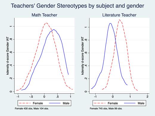
Teachers’ Implicit Gender Bias (IAT Measure) by Gender and Subject They Teach

This graph (color version available online) shows the distribution of Gender-Science IAT scores for math and literature teachers, separated by gender. A higher value of implicit bias indicates a stronger association between scientific-males and humanities-females. Zero indicates no gender stereotypes.

The richness of the data collected allows me to explore the determinants related to the reaction time to stimuli in the IAT score. Table III, Panel A shows that women teaching math have lower implicit stereotypes (column (1)), but age, education of own mother, and whether teachers have children do not have a statistically significant correlation with IAT scores (columns (2)–(5)). Gender stereotypical beliefs are rooted in cultural traits, transmitted from generation to generation (Guiso, Sapienza, and Zingales 2006). I find that exposure to cultural norms is strongly associated with the IAT score. Table III, Panel B, column (1) shows that implicit stereotypes are correlated with the place of birth of teachers: around 40% of math teachers in this sample are born in the south, where gender norms are stronger, as shown for instance by Campa, Casarico, and Profeta (2010).³¹ I investigate this aspect by providing evidence that women's labor force participation in the teachers' province of origin is negatively correlated with IAT score (Panel B, column (2)). As a proxy of cultural norms in the province of birth, I also use the answers to the World Value Survey question on the relative rights of men and women to paid jobs when jobs are scarce.³² I find a positive correlation between less conservative gender norms measured by this question and IAT scores (Panel B, column (3)). In the survey I administered, I asked the same question of teachers and found a low, and indistinguishable from 0, correlation (Panel B, column (4)). There may be social desirability bias in the self-reported measure when teachers are interviewed in the school. In Panel B, column (5) I correlate implicit bias and explicit beliefs about innate differences in ability between men and women and find a weak, yet indistinguishable from 0, correlation in the expected direction. This result is not surprising in light of findings in social psychology that implicit stereotypes often differ from explicit and self-reported stereotypes (Nosek, Banaji, and Greenwald 2002; Lane et al. 2007).

Table III

Correlation between Teachers’ Characteristics and Gender IAT Score

Dep. var.: raw IAT
Panel A: Independent variables (background teachers’ characteristics)
	Female	Age	High Mother Edu	Children	Daughters
	(1)	(2)	(3)	(4)	(5)
	−0.174***	−0.015	0.011	−0.072	0.035
	(0.051)	(0.020)	(0.035)	(0.105)	(0.047)
Obs.	454	454	454	454	454
R2	0.043	0.014	0.011	0.011	0.012
Panel B: Independent variables (cultural traits and beliefs)
	Born North	Women LFP	WVS City Born	WVS Indiv	Innate Ability
	(1)	(2)	(3)	(4)	(5)
	−0.081**	−0.295**	0.307***	−0.003	−0.028
	(0.035)	(0.146)	(0.110)	(0.047)	(0.046)
Obs.	454	433	389	454	454
R2	0.022	0.021	0.022	0.011	0.011
Panel C: Independent variables (education and teacher experience)
	STEM	Laude	Full Contract	Olympiad	High Exp
	(1)	(2)	(3)	(4)	(5)
	−0.060	−0.082**	−0.075	0.067	−0.016
	(0.045)	(0.039)	(0.053)	(0.069)	(0.063)
Obs.	454	454	454	454	454
R2	0.016	0.019	0.019	0.200	0.017

Notes. This table reports OLS estimates of the correlation between math teachers’ IAT score and own characteristics. The unit of observation is teacher t in school s. Standard errors (in parentheses) are robust and clustered at the school level. The number of clusters is 90. School fixed effects are included in all regressions. The significance and magnitude of coefficients are not affected by the inclusion of fixed effects. The variable “Female” indicates the gender of the teacher, “Born North ” assumes value 1 if the teacher was born in the north of Italy, “High Mother Edu” is a dummy that assumes value 1 if the mother of the teacher has at least a diploma, “Children” and “Daughters” are dummies that assume a value of 1 if the teacher has children/daughters. The variable “STEM” assumes value 1 if the teacher has a degree in math, engineering, or physics; “Laude” is a dummy that assumes value 1 if the degree was achieved with honors, “Full Contract” assumes value 1 if the teacher has tenure, “Olympiad” is 1 for teachers in charge of math Olympics in the school; “High Exp” is a dummy variable that assumes value 1 if the teacher has more than 15 years of experience; “Women LFP” is the labor force participation of women in the province of birth; “WVS City Born” is the WVS answer to the relative rights of men and women to paid jobs when jobs are scarce; “WVS Indiv” is the answer to the same question at the individual level, “Innate Ability” regards the teacher's belief about innate differences in math abilities between men and women (1 means no differences in innate ability, 0 otherwise). I include the order of IATs for math teachers and missing categories if the information is not available. ** and *** indicate significance at the 5% and 1% levels, respectively.

In Panel C, I correlate the IAT score with qualifications (type of degree and whether the degree was achieved with honors) and other proxies of quality of teachers (tenure, being the professor in charge of math Olympics in the school, and experience in teaching).³³ Point estimates are small and indistinguishable from 0, with the exception of achieving a degree with honors.³⁴ I also check whether the Gender-Science IAT score is correlated with the race IAT score. In the same regression as Table III, I find that the correlation is negative (−0.074 with standard error 0.123). Hence, math teachers more biased in one sphere are not more biased in the other sphere. The IAT score does not seem to capture a general “ability” in doing this type of test for math teachers.

Online Appendix Table A.IV shows all correlations presented in separate regressions in Table III together, for the sample of teachers whose data was matched with student outcomes (column (1)) and for all teachers who completed the survey (column (2)). Interestingly, the results are very similar. Finally, columns (3) and (4) provide evidence of the correlation between characteristics of literature teachers and their IAT score. As shown in Figure I, female literature teachers are more likely than male literature teachers to associate math-male and literature-female. This is by far the most relevant factor in explaining the IAT score of literature teachers.

IV.C. Exogeneity Assumption

Next I present evidence on the absence of a systematic correlation between teacher gender stereotypes and student characteristics. If parents are able to guess which teachers have more stereotyping behavior, they may try to (informally) affect class assignment of their daughters. Although this seems unlikely because implicit stereotypes are not an easily observable trait, it is also possible that parents try to select teachers according to characteristics correlated with IAT score, such as gender and place of birth. Furthermore, even if some parents manage to allocate their children to teachers with higher “quality,” it does not necessarily mean that they are less gender biased, as shown in Table III.³⁵

Table IV reports the correlation between student characteristics and stereotypes of math and literature teachers in Panels A and B, respectively. In Panel A, column (1), I provide evidence that girls are not systematically assigned to math teachers with stronger or weaker gender stereotypes than boys, while in column (2) I show that daughters of highly educated mothers are not less likely to be assigned to teachers with more stereotypes than those from lower socioeconomic backgrounds—the difference is not statistically significant and the point estimate goes in the opposite direction. In Panel A, columns (3) and (4), I analyze the correlation with paternal occupation and immigration background and I do not find a statistically significant correlation. The point estimates are very small in terms of magnitude, and the results are similar including all characteristics jointly (column (5)). The p-value for the F-test of overall significance of these variables is .379, suggesting that we cannot reject the joint null hypothesis at conventional levels. Finally, in the last column, I include the standardized test score in math in grade 5 before entering middle school despite the sample size being reduced substantially because of data availability issues.³⁶ The assumption of “as good as random” assignment of students to math teachers with different IAT scores within a school seems to be supported in this context. Panel B reports the correlations between the same student characteristics and literature teacher stereotypes. In this case, some point estimates are statistically different from 0 at conventional levels, even if they are small in magnitude and often in the opposite directions when all controls are jointly included in columns (5) and (6). Including these controls is potentially more relevant while analyzing the impact of literature teacher stereotypes. The results are identical when observations are collapsed at the teacher level, as shown in Online Appendix Table A.V.

Table IV

Exogeneity of Assignment of Students to Teachers with Different Bias

	(1)	(2)	(3)	(4)	(5)	(6)
Panel A: Dependent variable: implicit gender stereotypes of math teacher (standardized)
Female	−0.007	−0.015	−0.015	−0.009	−0.023	0.003
	(0.007)	(0.011)	(0.013)	(0.008)	(0.016)	(0.026)
High edu mother		−0.023			−0.022	−0.037*
		(0.015)			(0.014)	(0.022)
Fem * High edu mother		0.014			0.014	0.009
		(0.018)			(0.019)	(0.036)
Medium occupation father			−0.015		−0.009	0.043
			(0.015)		(0.014)	(0.031)
Fem * Medium occupation father			0.012		0.011	−0.041
			(0.020)		(0.020)	(0.042)
High occupation father			−0.028		−0.018	0.023
			(0.021)		(0.019)	(0.039)
Fem * High occupation father			0.002		−0.001	0.026
			(0.021)		(0.024)	(0.059)
Immigrant				0.008	0.006	0.033
				(0.018)	(0.018)	(0.030)
Fem * Immigrant				0.009	0.011	−0.004
				(0.019)	(0.020)	(0.038)
Std math 5						−0.013
						(0.013)
Fem * Std math 5						−0.019
						(0.020)
Obs.	30,359	30,359	30,359	30,359	30,359	6,847
R2	0.338	0.338	0.338	0.338	0.338	0.348
Panel B: Dependent variable: implicit gender stereotypes of literature teacher (standardized)
Female	0.014*	0.018	−0.008	0.008	−0.014	0.026
	(0.008)	(0.011)	(0.015)	(0.009)	(0.016)	(0.033)
High edu mother		0.004			0.009	−0.021
		(0.014)			(0.014)	(0.024)
Fem * High edu mother		−0.015			−0.026	−0.073**
		(0.017)			(0.018)	(0.036)
Medium occupation father			−0.031*		−0.039**	−0.013
			(0.017)		(0.018)	(0.034)
Fem * Medium occupation father			0.030		0.047**	0.038
			(0.022)		(0.023)	(0.046)
High occupation father			−0.007		−0.018	0.011
			(0.023)		(0.023)	(0.037)
Fem * High occupation father			0.036		0.058**	0.053
			(0.026)		(0.028)	(0.058)
Fem * Immigrant				0.031	0.041**	−0.007
				(0.020)	(0.020)	(0.042)
Immigrant				−0.017	−0.019	0.018
				(0.020)	(0.020)	(0.030)
Std reading 5						0.007
						(0.012)
Fem * Std reading 5						0.002
						(0.016)
Obs.	29,486	29,486	29,486	29,486	29,486	6,873
R2	0.344	0.345	0.345	0.345	0.345	0.417

Notes. This table reports OLS estimates of the correlation between teacher stereotypes measured by IAT score and student characteristics. The unit of observation is student i in class c taught by teacher t in grade 8 of school s. Standard errors (in parentheses) are robust and clustered at the teacher level. The variable “Fem” indicates the gender of the student, “High Edu Mother” assumes value 1 if the mother has at least a five-year high school diploma, “Medium occupation father” assumes value 1 if the father is a teacher or office worker, while “High occupation father” is 1 if the father is a manager, university professor, or executive. “Immigrant” assumes value 1 if the student is not an Italian citizen, while “Std math/reading 5” is the standardized test score in grade 5 in mathematics/reading. All regressions include controls for the order of IAT in the questionnaire administered. The last column has a lower number of observations because the test score in grade 5 is available only for part of the sample. The F-test for joint significance of all characteristics is 0.379 for Panel A (math teachers, column (5)) and 0.054 for Panel B (literature teachers, column (5)). * and **, indicate significance at the 10% and 5% levels, respectively.

The second aspect regards the absence of a systematic grouping of students by socioeconomic background and initial ability. Within schools, classes are formed by the principal with the main objective of creating comparable groups in terms of gender, ability, and socioeconomic background across classes, thereby guaranteeing heterogeneity within each class in the same school and cohort. This objective is spelled out in the official documents on the school websites and emerges from self-reported information from principals discussed in Online Appendix B. I have information about the observable characteristics of students that are used to create classes (gender, education and occupation of parents, immigration status, and generation of immigration). Plausibly, unobservable student characteristics are unknown to school principals at the moment of class formation, especially considering that students change all their teachers and school building when moving from elementary to middle school. I check whether class assignments are statistically independent of student characteristics with a series of Pearson chi-square tests. First, I consider the assignment of individual characteristics (gender, education and occupation of parents, immigration status, and generation of immigration). Then I check that within each characteristic, class assignment is statistically independent from gender. I find that in less than 10% of the tests performed, the p-value is lower than or equal to 5%. There is no evidence of strong systematic grouping of students according to their socioeconomic background. In Section V.A, I provide evidence on the robustness of the main results. First, I do a permutation test where I randomly assign stereotypes to teachers. Second, I restrict the data set to classes where assignment to peers is statistically independent for all student characteristics by gender.

1. Timing of IAT Collection

Teachers’ gender stereotypes were collected between October 2016 and March 2017, and they are matched with data of students who graduated from middle school between June 2012 and June 2017 (the detailed timeline is available in Figure II). An advantage of exploiting data of students who graduated before their teachers did the survey is that taking the IAT or knowledge about this study could not have affected students’ performance or teachers’ or parents’ attention to the issue of gender stereotypes for the cohorts of students graduating before 2017. A potential concern is that IAT scores may be affected by exposure to the same cohorts of students. Indeed, the IAT is expected to be the combination of a trait stable over time, capturing individual stereotypes, and occasion-specific variation and noise that may be affected by conditions while taking the test, and stimuli received by the subject in the period right before the test.³⁷

Figure II

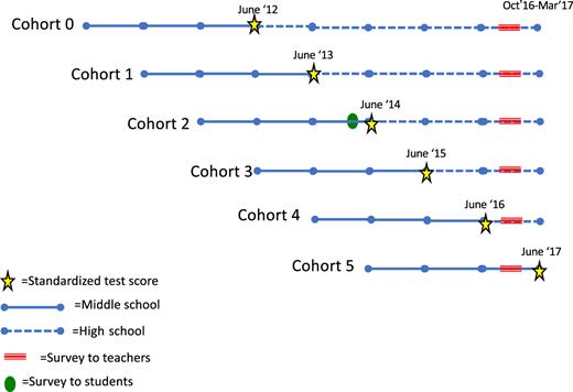
Timeline of Main Data Available for Students and Teachers

This figure shows the timeline of data collected for the three cohorts of students. They graduated from middle school between 2012 and 2017. Teachers were surveyed between October 2016 and March 2017. Standardized tests are administered at the end of grade 8.

Reverse causality seems unlikely for several reasons. I can provide supporting evidence against this issue by showing that the results are unchanged when I restrict the sample to the last cohort of students who graduated after their teachers took the IAT (results are presented in Section V.A). Furthermore, teachers with more stereotypes are not systematically assigned to students with different characteristics, such as family background and standardized test scores in math (see Table IV and Online Appendix Table A.V). Teachers included in our analysis have been teaching, on average, for 20 years (with a median of 22 years) and therefore over time they were exposed to hundreds of students.

V. The Impact of Teachers’ Implicit Stereotypes

V.A. Performance in Math

Table V shows the effect of teachers’ implicit stereotypes on the gender gap in standardized test scores in grade 8 within the class, presenting the results of estimating equation (1). I document the impact of math and literature teachers in Panels A and B, respectively. By the age of 14, girls lag 0.18 standard deviations behind in math compared to their male classmates (Table V, Panel A, column (1)).³⁸ Classes that are assigned to teachers with a 1 standard deviation higher IAT score during the three years of middle school have a 0.032 standard deviation larger gender gap in math performance in grade 8.³⁹ Column (3) includes student characteristics |$(\mathbf {X}_{i})$|⁠, and column (4) adds their interaction with gender of the children, without affecting the coefficient of interest.

Table V

Estimation of the Effect of Teachers’ Gender Stereotypes on Standardized Test Score in Grade 8: Class FE Regression

	(1)	(2)	(3)	(4)	(5)
Panel A: Dependent variable: math standardized test score in grade 8
Female	−0.184***	−0.198***	−0.198***	−0.174***	−0.032
	(0.012)	(0.013)	(0.012)	(0.025)	(0.082)
Fem * Math teacher stereotypes		−0.032**	−0.031***	−0.032***	−0.031***
		(0.013)	(0.012)	(0.012)	(0.011)
Fem * Teacher fem					0.020
					(0.030)
Fem * Teacher born north					0.010
					(0.024)
Fem * Advanced STEM teacher					−0.006
					(0.024)
Gender gap	−0.185	−0.185	−0.186	−0.186	−0.1856
Obs.	30,359	30,359	30,359	30,359	30,359
R2	0.206	0.206	0.275	0.275	0.276
Panel B: Dependent variable: reading standardized test score in grade 8
Female	0.221***	0.225***	0.221***	0.226***	0.307***
	(0.012)	(0.013)	(0.012)	(0.024)	(0.093)
Fem * Lit teacher stereotypes		−0.012	−0.006	−0.007	−0.001
		(0.013)	(0.012)	(0.012)	(0.013)
Fem * Teacher fem					−0.044
					(0.039)
Fem * Teacher born north					0.011
					(0.027)
Gender gap	0.221	0.221	0.219	0.219	0.219
Obs.	29,486	29,486	29,486	29,486	29,486
R2	0.181	0.181	0.291	0.291	0.291
Class FE	Yes	Yes	Yes	Yes	Yes
Student controls	No	No	Yes	Yes	Yes
Student controls * Fem	No	No	No	Yes	Yes
Teacher controls * Fem	No	No	No	No	Yes

Notes. This table reports OLS estimates of equation (1), where the dependent variable is math or reading standardized test score in grade 8 in Panels A and B, respectively, and the dependent variables refer to math teachers in Panel A and literature teachers in Panel B. The unit of observation is student i in class c taught by teacher t in grade 8 of school s. Standard errors (in parentheses) are robust and clustered at the teacher level (454 in Panel A and 615 in Panel B). The variable “Fem” indicates the gender of the student. Individual controls include education of the mother, occupation of the father, immigrant dummy, generation of immigration, and their interactions with the gender of the student. Teacher controls include the interaction between student gender and teacher gender, place of birth, age, children and daughters, advanced STEM degree (physics, math, engineering), leader of school math Olympics, degree with honors, refresher courses, type of contract, and education of the teacher’s mother. ** and ***, indicate significance at the 5% and 1% levels, respectively.

Although the level of teacher stereotypes and all characteristics are absorbed by the class fixed effect, column (5) includes the interaction between student gender and teacher characteristics |$(\mathbf {Z}_{c})$|⁠. The magnitude and significance of the coefficient of interest (Fem * Teacher Stereotypes) is not affected when all these interaction effects are absorbed. Observable characteristics of teachers, interacted with students’ gender, are not driving the relation between gender gap and teacher stereotypes. I report the coefficients only for the main characteristics, but the effects are mainly small and insignificant at conventional levels for all variables, including age, parents’ education, whether the teacher has daughters, whether he or she achieved the degree with honors, the type of teaching contract, refresher courses, and appointment as teacher in charge of math Olympics. Ceteris paribus, female students assigned to female teachers have slightly (albeit insignificantly) higher math performance in grade 8 compared with their classmates.⁴⁰ The absence of a differential impact on boys and girls of teacher gender is consistent with the result of Bharadwaj et al. (2016). However, other studies find that having a teacher of the same gender helps improve performance, especially at the college level (Dee 2005; Carrell, Page, and West 2010). In Online Appendix Table A.VI, I split the sample by teacher gender. The point estimate shows that the impact of teachers’ implicit stereotypes on student performance is slightly larger in terms of magnitude for male, compared to female, teachers. However, what seems to matter the most is whether the teacher has gender stereotypes.

To give a clearer interpretation, Online Appendix Table A.VII, columns (1)–(3) show the impact on the gender gap in the class of being assigned to a teacher with a positive (“boys-math” association) or a negative score (“girls-math” association) on the IAT test. The gender gap in the classroom is around 0.15 std. dev. for students assigned to a teacher with an IAT score greater than 0, and it increases by one third (0.20 std. dev.) for classes assigned to a teacher with an IAT score lower than 0. In columns (4)–(6), I consider the thresholds defined by Greenwald, Nosek, and Banaji (2003), where “no stereotypes” is the interval of IAT raw score between −0.15 and +0.15, while “boys-math” and “girls-math” indicate a stronger association of the scientific field with male and female names, respectively. Most of the difference in the gap is driven by being assigned to a teacher with a “boys-math” attitude or with “no systematic associations” (75% of teachers) compared to a teacher with a “girls-math” attitude (25% of teachers).

Are teachers with stronger stereotypes worse instructors or are they helping boys learn math? I investigate the effect of teacher bias by estimating equation (2) directly, comparing students of the same gender within the same school and cohort but assigned to different classes. Figure III shows that having a teacher with a strong “boys-math” attitude has a negative effect on female students, while a “girls-math” attitude has a positive impact on math improvements of girls. The linear approximation presented in Table V seems to adequately represent the data. There is no statistically significant impact on male students throughout the whole distribution of teachers’ IAT scores. Table VI, column (5) mirrors Figure III: it presents the results of the regression analysis and shows that girls are lagging behind when assigned to teachers with stronger implicit associations, while boys are not affected by teacher stereotypes. The results are robust to the inclusion of the controls as in Table V. In this specification, the characteristics of teachers are not absorbed by class fixed effects and therefore controls at the teacher level are particularly relevant and column (5) is the preferred specification.

Figure III

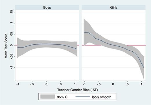
Effect of Teacher Bias on Student Math Performance by Gender

This figure shows the effect of teacher stereotypes on student achievement by gender. The variable on the y-axis is the residualized standardized test score in grade 8, after controlling for school by cohort fixed effects, and student- and teacher-level controls. The variable on the x-axis is the raw IAT score. A higher value of implicit bias indicates a stronger association between scientific-males and humanistic-females. The regression includes student and teacher controls.

Table VI

Estimation of the Effect of Teachers’ Gender Stereotypes on Math Standardized Test Score in Grade 8: School FE Regression

	(1)	(2)	(3)	(4)	(5)
Dependent variable: math standardized test score in grade 8
Female	−0.180***	−0.192***	−0.196***	−0.166***	−0.047
	(0.012)	(0.013)	(0.012)	(0.024)	(0.079)
Fem * teacher stereotypes		−0.029**	−0.029**	−0.031***	−0.030***
		(0.012)	(0.011)	(0.011)	(0.011)
Teacher stereotypes		−0.018	−0.015	−0.014	−0.013
		(0.013)	(0.012)	(0.012)	(0.012)
Teacher fem					0.066**
					(0.033)
Fem * teacher fem					0.018
					(0.030)
Teacher born north					−0.006
					(0.025)
Fem * teacher born north					0.012
					(0.023)
Advanced STEM					−0.048*
					(0.027)
Fem * advanced STEM teacher					−0.006
					(0.024)
Gender gap	−0.180	−0.180	−0.184	−0.184	−0.184
School, year FE	Yes	Yes	Yes	Yes	Yes
Student controls	No	No	Yes	Yes	Yes
Student controls* fem	No	No	No	Yes	Yes
Teacher controls	No	No	No	No	Yes
Obs.	30,359	30,359	30,359	30,359	30,359
R2	0.128	0.129	0.208	0.208	0.214

Notes. This table reports OLS estimates of equation (2), where the dependent variable is math standardized test score in grade 8. The unit of observation is student i in class c taught by teacher t in grade 8 of school s. Standard errors (in parentheses) are robust and clustered at the teacher level. The number of clusters is 454. The number of fixed effects (school by cohort) is 459. The variable “Fem” indicates the gender of the student. Individual controls include education of the mother, occupation of the father, immigrant dummy, generation of immigration, and their interactions with the gender of the student. Teacher controls include teacher gender, place of birth, children and daughters, advanced STEM degree (physics, math, engineering), leader of school math Olympics, degree with honors, refresher courses, age, type of contract, education of the teacher’s mother and the interaction with student gender of all these characteristics. *, **, and *** indicate significance at the 10%, 5%, and 1% levels, respectively.

1. Heterogeneous Effects: Student Ability and Interaction Time with Teachers

I examine which students are the most affected by teacher stereotypes, considering their background characteristics and the time of exposure to their teachers. Online Appendix Table A.VIII shows that the effect of implicit stereotypes is stronger for female students who started middle school at the middle or lower end of the initial ability distribution. Based on the estimates in column (2), a 1 standard deviation increase in teacher bias leads to −0.095 standard deviation lower performance among girls in the lowest tercile of test scores in grade 6, −0.068 (standard error 0.01) and +0.040 (standard error 0.22) for those girls in the middle and top terciles, compared to boys in the same initial tercile.⁴¹ There are no significant heterogeneous effects according to other background characteristics, such as mothers’ education or whether the student is an immigrant.⁴²

Why do girls with lower level of ability initially suffer the most from the interaction with biased teachers? The empirical evidence presented is consistent with the stereotype threat model (Steele and Aronson 1995): individuals with higher risk of conforming to the predicament that “women are bad at math” are those more deeply affected. Indeed, male students are not influenced by teacher stereotypes and, among girls, those most strongly affected have lower initial math achievement and are at higher risk of confirming the negative expectations of their group. Online Appendix E presents a conceptual framework that illustrates how teacher stereotypes can differentially affect effort and outcomes of students at the bottom and the top of the ability distribution.⁴³ One complementary explanation, consistent with the interaction theory (McConnell and Leibold 2001), is that female students with higher initial math achievement may need less interaction with their math teacher to avoid lagging behind with their peers. This result is also consistent with evidence from Tiedemann (2002): teachers’ perception of the math ability of their students is biased mainly toward average and low-achieving female students who are perceived as less talented compared with their actual performance.

To investigate this further, I analyze the differential effect according to the quantity of interaction time between a teacher and their students. The last two columns of Online Appendix Table A.VIII analyze whether there are heterogeneous effects in terms of years of exposure and hours each week.⁴⁴ Furthermore, I exploit the fact that around 25% of classes did not have the same teacher for all three years of middle school.⁴⁵ For both variables, I do not see a statistically significant pattern, but the point estimates suggest that longer exposure substantially increases the gender gap in the classroom. After three years of exposure, girls are lagging 0.037 standard deviations behind compared with their male classmates, while the effect is only 0.006 for those who changed teacher (column (6)). Consistent with this result, Online Appendix Table A.IX shows the impact of one year or less of exposure to teachers’ implicit stereotypes. I exploit two different samples. First, I use test score in grade 6, administered a few months after assignment to middle school teachers (columns (1)–(3)) and collected only up to 2012–13 and reported only for those teachers who took the test in 2017. Second, I exploit the fact that some classes were assigned to a new teacher at the beginning of grade 8 (columns (4)–(6)). In both cases, the point estimates are indistinguishable from 0.

2. Robustness Checks

First, even if all students are supposed to take the standardized test in grade 8, I am missing information on the grade for 7% of students.⁴⁶ This mismatch may be due to some students not attending the test or schools misreporting the code to match data from the Ministry of Education and the code of the standardized test score with INVALSI. Online Appendix Table A.X shows that girls are around 2.5 percentage points less likely to have missing test scores than boys, but the effect is not statistically different for classes assigned to teachers with higher or lower level of stereotypes.

Second, in Online Appendix Table A.XI, I show the effect of the main specification presented in Table V separately by cohorts of students who graduated before teachers took the IAT (school years 2012–2016) and for the cohort of students who graduated after teachers took the IAT (school year 2017). Reassuringly for the potential reverse causality concerns expressed in Section IV.C, results are statistically indistinguishable and the point estimate is larger for the last cohort of students.⁴⁷

Third, Online Appendix Figure A.V plots the coefficient “Fem * Stereotypes” from a permutation test that runs the main regression in equation (1) 1,000 times randomly assigning the stereotypes to math teachers. In 5 out of 1,000 permutations, I find a coefficient smaller than the one in Table V. Finally, in Online Appendix Table A.XII, I restrict the sample to schools by cohorts where Pearson chi-square tests suggest statistical independence of all student characteristics (gender, education of the mother, occupation of the father, immigrant dummy, generation of immigration) and of all student characteristics by gender. In this additional robustness check, results are also not affected.

V.B. Performance in Reading

Girls outperform boys in reading by 0.22 standard deviations (Table V, Panel B, column (1)): the gender gap in female-typed areas is reversed compared to the one in male-typed areas discussed in the previous section, similarly to most OECD countries (Fryer and Levitt 2010). Table V, Panel B focuses on the impact of literature teacher stereotypes on reading performance. Although the point estimate is negative, the gender stereotypes of literature teachers do not statistically significantly affect this gap. Online Appendix, Table A.VI, Panel B shows that the negative point estimate is mainly driven by male teachers, but even for this subsample of teachers, the effect is not statistically significant at conventional levels.⁴⁸

Online Appendix Table A.XIII investigates the impact of teacher stereotypes, considering the implicit IAT of literature and math teachers and restricting the sample to those classes for which these scores are jointly available. The implicit stereotypes of literature teachers do not have a significant impact on math (columns (1)–(4)) or on reading standardized test scores (columns (5)–(8)). The inclusion of their IAT scores does not affect the negative and statistically significant effect of math teachers’ stereotypes on math performance. Indeed, being assigned to a math teacher with stronger implicit stereotypes seems to have a negative, although indistinguishable from 0, effect on performance in reading, suggesting that female students do not simply substitute their effort in math for more effort devoted to studying literature.

There are several potential explanations for these results. First, it could be due to a measurement issue. Improvements in math may be easier to detect and measure on multiple choice tests. Standardized test scores in reading may be less elastic in capturing improvements during middle school, after basic literacy is completed, while standardized test scores in math may be closely related to specific learning during more recent school years. A significant impact on math standardized test scores accompanied by no impact or a smaller impact in reading is a common result in the literature (Bettinger 2012; Levitt et al. 2016; Carlana, La Ferrara, and Pinotti 2018). Furthermore, Gender-Science IAT scores do not allow one to distinguish between the stereotype that women are bad at math and men are bad at reading. If the former association is more salient, this test may be better at detecting stereotypes in the scientific field and therefore it may have higher predictive power for math. Second, students may need less support and interaction with their math teachers compared to their literature teachers to perform well on the respective tests. Both math and literature teachers with stronger implicit associations may end up interacting less (in terms of quantity or quality) with students of the stigmatized group, which is consistent with findings on the role of interaction between managers and minority workers by Glover, Pallais, and Pariente (2017). However, only girls may be negatively affected because in math the support and explanation of teachers may be crucial for learning. Third, math skills are likely to be mainly taught in school, whereas reading is more likely to be supplemented by parents or other caregivers at home. Hence, teacher stereotypes may matter more in subjects almost exclusively taught by teachers versus other adults. Finally, consistent with Kugler, Tinsley, and Ukhaneva (2017) and Große and Riener (2010), girls may be more vulnerable to the gender stereotype that women are bad at math compared to boys exposed to the gender stereotype that men are bad at reading.⁴⁹ Girls tend to be less likely to believe that their good performance is due to their talent and more likely to believe that it is due to their effort. This is disproportionately true for math performance, as I show in Online Appendix D.

V.C. Choice of High School Track and Teachers’ Recommendation

1. Background

High school track choice is the first crucial career decision in the Italian schooling system. There are three main types of high school: academic, technical, and vocational.⁵⁰ Within the academic track, the scientific and classical subtracks are top-tier. As shown in Table II, there are substantial gender differences in the type of track selected: the preferred choices among girls are academic tracks related to psychology, languages, and art, whereas boys’ preferred choices are academic scientific and technical technological tracks.

Each family receives a formal letter from the school with the subtrack recommended by the teachers, mainly driven by math and literature teachers who interact the most with students at school.⁵¹ Students and their families are free to choose their most preferred track, with no constraints based on grades or teachers’ official track recommendation. Table II documents that girls are less likely, on average, to be recommended to the vocational track (7 percentage points) and scientific track (4 percentage points) than boys.⁵² In the survey to teachers, I directly ask which factors they mainly consider when giving the track recommendation (see Online Appendix C.2 for the specific question). Both math and literature teachers consider motivation and interest as the most important factors, followed by grades given to students and involvement of parents in school activities. Given that girls tend to have higher academic motivation,⁵³ the evidence on fewer recommendations toward vocational school for girls is not surprising.

Online Appendix Table A.XIV shows that track choice and teachers’ track recommendation are correlated for vocational high school (columns (1)–(3)) and scientific high school (columns (4)–(6)), with the latter correlation being substantially stronger. This table underscores some interesting gender differences: girls are 10 percentage points more likely to follow their teachers’ recommendation to vocational track, which implies a 31% increase with respect to boys, and both genders are equally likely to follow a recommendation to scientific track.

In this section, I explore the impact of teacher stereotypes on track choice at the end of middle school using an ordered logit, and then I focus on the choice of the vocational track and scientific academic track using a linear probability model.⁵⁴

2. Results

Table VII, Panel A reports fixed effects ordered logit estimates using the BUC estimator (Baetschmann, Staub, and Winkelmann 2015), in which the dependent variable assumes value 1 for the vocational track, value 2 for intermediate tracks (technical and non top–tier academic), and value 3 for top-tier high school (scientific and classical). These three categories are created grouping students according to their average test scores in grade 8 (before tracking), as can be clearly seen in Online Appendix Figure A.VI.⁵⁵ As shown in column (2), stereotypes of math teachers have a negative and statistically significant effect on the choice of a better high school for girls, and the effect is unchanged by the inclusion of student- and teacher-level controls (columns (3) and (4), respectively). Although all students are supposed to take the test, those who go to high school without taking the test are disproportionately represented among students enrolled in the vocational track.⁵⁶ When I restrict the sample to students who actually attended the standardized test in grade 8, the impact of teacher stereotypes on track choice is substantially smaller and insignificant at the conventional level (column (5)). In column (6), I include the quadratic of the math standardized test score in grade 8, as a potential mediator given the results in Section V.A. Including these controls does not affect the point estimate.

Table VII

Estimation of the Effect of Teachers’ Gender Stereotypes on High School Track Choice: Ordered Logit with Class FE Regression

	(1)	(2)	(3)	(4)	(5)	(6)	(7)	(8)
Panel A: Dependent variable: high school track choice
Fem	−0.270***	−0.300***	−0.306***	−0.458**	−0.483**	−0.496**	−0.370***	−0.292***
	(0.028)	(0.030)	(0.030)	(0.219)	(0.231)	(0.237)	(0.048)	(0.032)
Fem * math teacher stereotypes		−0.074**	−0.070**	−0.059*	−0.035	−0.035	−0.094**
		(0.031)	(0.030)	(0.030)	(0.032)	(0.034)	(0.042)
Fem * lit teacher stereotypes							0.028	0.011
							(0.045)	(0.031)
Individuals	21,027	21,023	20,750	20,725	17,899	17,016	11,192	20,254
Obs.	47,351	47,351	47,351	47,351	41,772	41,772	25,395	45,167
Pseudo-log-likelihood	−21,026	−21,022	−20,749	−20,724	−17,896	−17,012	−11,191	−20,029
Panel B: Dependent variable: high school track recommendation
Fem	0.179***	0.151***	0.148***	0.137	0.201	0.406	0.063	−0.190***
	(0.032)	(0.035)	(0.036)	(0.269)	(0.281)	(0.301)	(0.054)	(0.036)
Fem * math teacher stereotypes		−0.068**	−0.046	−0.059	−0.059	−0.046	−0.077
		(0.031)	(0.035)	(0.037)	(0.037)	(0.044)	(0.048)
Fem * lit teacher stereotypes							0.041	0.006
							(0.051)	(0.036)
Individuals	18,684	18,684	18,684	18,684	16,904	16,904	10,575	17,979
Obs.	39,349	39,349	39,349	39,349	34,215	34,215	21,789	38,048
Pseudo-log-likelihood	−17,042	−17,039	−15,241	−15,222	−13,547	−10,375	−9,711	−16,623
Class FE	Yes	Yes	Yes	Yes	Yes	Yes	Yes	Yes
Student controls	No	No	Yes	Yes	Yes	Yes	No	No
Student controls * fem	No	No	No	Yes	Yes	Yes	No	No
Teacher controls * fem	No	No	No	Yes	Yes	Yes	No	No
Sq. math test 8	No	No	No	No	No	Yes	No	No

Notes. This table reports fixed effects ordered logit estimates (BUC estimators following Baetschmann, Staub, and Winkelmann (2015), where the dependent variable assumes value 1 for vocational track, value 2 for intermediate tracks (technical and no top-tier academic), and value 3 for top-tier high school (scientific and classical). The unit of observation is student i in class c taught by teacher t in grade 8 of school s. Standard errors (in parentheses) are robust and clustered at the class level. Columns (5) and (6) restrict the sample only to those students with a standardized test score in grade 8, while column (7) includes only students for whom we have information about both the math and literature teacher. The variable “Fem” indicates the gender of the student and “Stereotypes” is the IAT score of the teacher. Individual controls include education of the mother, occupation of the father, immigrant dummy, generation of immigration, and their interactions with the gender of the student. Teacher controls include the interaction between student gender and teacher gender, place of birth, children and daughters, advanced STEM degree (physics, math, engineering), leader of school math Olympics, degree with honors, refresher courses, age, type of contract, and education of the teacher’s mother. “Sq. math test 8” is the second-order polynomial of test score in grade 8. “Obs.” denotes the number of student-choices in the estimation sample; “Individuals” denotes the number of unique people in the estimation sample. *, **, and *** indicate significance at the 10%, 5%, and 1% levels, respectively.

The last two columns of Table VII, Panel A provide evidence of the absence of a statistically significant impact on track choice of literature teachers. This result seems to support the idea that girls may be more vulnerable to the gender stereotypes of their math teachers compared to boys to the gender stereotypes of their literature teachers. Table VII, Panel B documents a similar pattern in terms of magnitude for teachers’ track recommendation, although estimates are less precise and indistinguishable from 0 when controls are included.

To delve deeper into the choice of the field of study, I provide evidence on the effect of teacher stereotypes at the bottom (vocational track) and the top (scientific track) of the ability distribution using a linear probability model and following the same structure of Table VII.⁵⁷ Girls are slightly more likely to attend a vocational track (1.2 percentage points) than boys, and they are 8.9 percentage points less likely to attend a scientific track, as shown in Table VIII, Panels A and B, column (1). This gap slightly increases when we include student-level controls (column (3)).⁵⁸ Consistently with the result in Table VII, math teacher stereotypes have a strong positive and statistically significant impact on the choice of vocational track for girls, with respect to boys in the same class. One standard deviation higher teacher stereotypes increases the probability of attending a vocational track for girls (with respect to boys) by around 2 percentage points, which corresponds to an increase of 11.4% with respect to the mean probability of attending vocational training for girls. When I restrict the sample to students who took the standardized test score in grade 8, the point estimate decreases by around one-third and is no longer statistically significant at the conventional level (Panel A, column (5)). The effect is mainly driven by students who did not take the test score in grade 8. Column (6) shows that including the squared polynomial of standardized test score absorbs most of the residual effect of math teacher stereotypes on the choice of vocational track. The last two columns of Table VIII show that literature teacher stereotypes have no significant effect on track choice.

Table VIII

Estimation of the Effect of Teachers’ Gender Stereotypes on High School Track Choice: Class FE Regression

	(1)	(2)	(3)	(4)	(5)	(6)	(7)	(8)
Panel A: Dependent variable: vocational high school track choice
Fem	0.012**	0.020***	0.019***	0.054	0.038	0.028	0.026***	0.011*
	(0.006)	(0.007)	(0.006)	(0.047)	(0.047)	(0.045)	(0.010)	(0.006)
Fem * math teacher stereotypes		0.019***	0.016**	0.013**	0.008	0.004	0.023**
		(0.007)	(0.007)	(0.007)	(0.007)	(0.006)	(0.009)
Fem * lit teacher stereotypes							0.009	−0.001
							(0.009)	(0.006)
Constant	0.163***	0.163***	0.190***	0.162***	0.180***	0.159***	0.153***	0.160***
	(0.003)	(0.003)	(0.008)	(0.010)	(0.010)	(0.010)	(0.004)	(0.003)
Mean Y fem	0.175	0.175	0.202	0.202	0.202	0.202	0.172	0.171
Obs.	21,015	21,015	21,015	21,015	19,506	19,506	11,302	20,254
R2	0.116	0.117	0.161	0.164	0.154	0.220	0.116	0.116
Panel B: Dependent variable: scientific high school track choice
Fem	−0.089***	−0.093***	−0.091***	−0.003	−0.012	−0.006	−0.107***	−0.092***
	(0.007)	(0.008)	(0.008)	(0.051)	(0.054)	(0.051)	(0.012)	(0.008)
Fem * math teacher stereotypes		−0.009	−0.006	−0.008	−0.008	−0.006	−0.024**
		(0.007)	(0.007)	(0.007)	(0.008)	(0.007)	(0.010)
Fem * lit teacher stereotypes							0.002	−0.006
							(0.011)	(0.007)
Constant	0.283***	0.283***	0.196***	0.164***	0.160***	0.122***	0.281***	0.284***
	(0.003)	(0.003)	(0.008)	(0.010)	(0.011)	(0.010)	(0.005)	(0.004)
Mean Y fem	0.194	0.194	0.107	0.107	0.108	0.108	0.185	0.191
Obs.	21,015	21,015	21,015	21,015	19,506	19,506	11,302	20,254
R2	0.117	0.117	0.152	0.159	0.161	0.273	0.111	0.116
Class FE	Yes	Yes	Yes	Yes	Yes	Yes	Yes	Yes
Student controls	No	No	Yes	Yes	Yes	Yes	No	No
Student controls * fem	No	No	No	Yes	Yes	Yes	No	No
Teacher controls * fem	No	No	No	Yes	Yes	Yes	No	No
Sq. math test 8	No	No	No	No	No	Yes	No	No

Notes. This table reports OLS estimates of equation (1), where the dependent variable is the high school track choice. The unit of observation is student i in class c taught by teacher t in grade 8 of school s. Standard errors (in parentheses) are robust and clustered at the class level. Columns (5) and (6) restrict the sample only to those students who took the standardized test in grade 8, while column (7) includes only students for whom we have information about both the math and literature teacher. The variable “Fem” indicates the gender of the student and “Stereotypes” is the IAT score of the teacher. Individual controls include education of the mother, occupation of the father, immigrant dummy, generation of immigration, and their interactions with the gender of the student. Teacher controls include the interaction between student gender and teacher gender, place of birth, children and daughters, advanced STEM degree (physics, math, engineering), leader of school math Olympics, degree with honors, refresher courses, age, type of contract, and education of the teacher’s mother. “Sq. math test 8 ” is the second-order polynomial of test score in grade 8. *, **, and *** indicate significance at the 10%, 5%, and 1% levels, respectively.

Table VIII, Panel B reports the OLS estimates for the probability of attending a scientific track. The impact of both math and literature teacher stereotypes is statistically indistinguishable from 0, although the point estimate is negative and close to 1 percentage point for math teachers.⁵⁹

Online Appendix Table A.XV shows the results estimating equation (2), with school by cohort (instead of class) fixed effects. Column (2) confirms the previous evidence of an impact on female students of math teacher stereotypes in terms of choice of vocational training. Part of the gender gap within class captured in the specification using class fixed effects is due to the lower probability of boys choosing the vocational track when assigned to teachers with stronger gender stereotypes.

Table IX provides evidence of a similar pattern compared to Table VIII in terms of magnitude of the effect of math and literature teacher stereotypes on track recommendation for vocational (Panel A) and scientific (Panel B) paths, although the effect is generally slightly smaller and less precisely estimated compared to the one on track choice. Track recommendation is a joint decision of the math and literature teacher, so own bias may be attenuated. Online Appendix Table A.XVI includes school-by-cohort fixed effects and suggests that girls may be slightly less likely to be recommended to the scientific track, even if the result is not robust to the inclusion of all sets of controls.

Table IX

Estimation of the Effect of Teachers’ Gender Stereotypes on High School Track Recommendation of Teachers: Class FE Regression

	(1)	(2)	(3)	(4)	(5)	(6)	(7)	(8)
Panel A: Dependent variable: vocational high school track recommendation
Fem	−0.074***	−0.067***	−0.062***	−0.074	−0.087	−0.110*	−0.053***	−0.082***
	(0.008)	(0.009)	(0.008)	(0.062)	(0.064)	(0.057)	(0.013)	(0.009)
Fem * Math teacher stereotypes		0.018**	0.011	0.012	0.011	0.004	0.018
		(0.009)	(0.008)	(0.008)	(0.009)	(0.008)	(0.012)
Fem * Lit teacher stereotypes							−0.000	0.006
							(0.013)	(0.009)
Constant	0.433***	0.433***	0.517***	0.516***	0.528***	0.470***	0.423***	0.429***
	(0.004)	(0.004)	(0.009)	(0.012)	(0.013)	(0.011)	(0.005)	(0.004)
Mean Y fem	0.359	0.359	0.450	0.450	0.450	0.450	0.362	0.349
Obs.	18,684	18,684	18,684	18,684	16,904	16,904	10,575	17,979
R2	0.143	0.143	0.271	0.272	0.244	0.427	0.132	0.138
Panel B: Dependent variable: scientific high school track recommendation
Fem	−0.031***	−0.034***	−0.035***	−0.054	−0.055	−0.046	−0.044***	−0.035***
	(0.006)	(0.006)	(0.006)	(0.047)	(0.051)	(0.047)	(0.011)	(0.007)
Fem * Math teacher stereotypes		−0.007	−0.004	−0.007	−0.007	−0.005	−0.013
		(0.007)	(0.007)	(0.007)	(0.007)	(0.007)	(0.009)
Fem * Lit teacher stereotypes							0.002	−0.001
							(0.011)	(0.007)
Constant	0.196***	0.196***	0.124***	0.106***	0.109***	0.080***	0.198***	0.203***
	(0.003)	(0.003)	(0.006)	(0.007)	(0.008)	(0.008)	(0.004)	(0.003)
Mean Y fem	0.165	0.165	0.090	0.090	0.091	0.091	0.160	0.168
Obs.	18,684	18,684	18,684	18,684	16,904	16,904	10,575	17,979
R2	0.235	0.235	0.278	0.280	0.283	0.402	0.201	0.219
Class FE	Yes	Yes	Yes	Yes	Yes	Yes	Yes	Yes
Student controls	No	No	Yes	Yes	Yes	Yes	No	No
Student controls * Fem	No	No	No	Yes	Yes	Yes	No	No
Teacher controls * Fem	No	No	No	Yes	Yes	Yes	No	No
Sq. Math Test 8	No	No	No	No	No	Yes	No	No

Notes. This table reports OLS estimates of equation (1), where the dependent variable is the high school track recommendation of teachers. The unit of observation is student i in class c taught by teacher t in grade 8 of school s. Standard errors (in parentheses) are robust and clustered at the class level. Columns (5) and (6) restrict the sample only to those students who took the standardized test in grade 8, while column (7) includes only students for whom we have information about both the math and literature teacher. The variable “Fem” indicates the gender of the student, and “Stereotypes” is the IAT score of the teacher. Individual controls include education of the mother, occupation of the father, immigrant dummy, generation of immigration, and their interactions with the gender of the student. Teacher controls include the interaction between student gender and teacher gender, place of birth, children and daughters, advanced STEM degree (physics, math, engineering), leader of school math Olympics, degree with honors, refresher courses, age, type of contract, and education of the teacher’s mother. “Sq. math test 8 ” is the second-order polynomial of test score in grade 8. *, **, and *** indicate significance at the 10%, 5%, and 1% levels, respectively.

To sum up, math teacher stereotypes have a substantial impact on track choice mainly by inducing more girls to self-select into the vocational track. The effect is driven by students at the bottom of the ability distribution or with missing data on test scores. The impact on scientific track is negative, but generally indistinguishable from 0. The scientific track is chosen by girls with high achievement test scores whose performance was not affected by teacher bias, as shown in the analysis of heterogeneous effects in Section V.A. Girls at the top of the math ability distribution are likely to have other academic-oriented role models in addition to their math teacher and a lower vulnerability to gender stereotypes. The result on track choice mirrors an analogous difference in teachers’ track recommendation, though it is smaller in magnitude and less precisely estimated. Literature teacher stereotypes have no significant effects on track choice of boys or girls. As discussed already, a potential explanation is that girls may be more vulnerable to the gender stereotypes of their math teachers compared to boys to the gender stereotypes of their literature teachers.

VI. Discussion of a Potential Mechanism: Self-Confidence

Self-confidence may play a crucial role in affecting performance, especially in “gender incongruent areas,” such as math for girls or literature for boys (Coffman 2014). According to findings in social psychology, the development of academic self-concept begins in childhood and is strongly influenced in the period after elementary school by stereotypes communicated by parents and teachers (Ertl, Luttenberger, and Paechter 2017). Students may believe that their own signal of ability and the signal received by teachers carry relevant information. However, if the signal received from teachers is biased by gender stereotypes, female students, for example, may develop a lower self-assessment of their ability in the scientific field and potentially invest less in their STEM education. This idea is consistent with the stereotype threat theory developed in the social psychological literature (Steele and Aronson 1995), according to which individuals at risk of confirming widely known negative stereotypes reduce their confidence and underperform in fields in which their group is ability-stigmatized (Spencer, Steele, and Quinn 1999). In Online Appendix E, I present a conceptual framework that develops the intuition for the stereotype threat theory.⁶⁰

Table X assesses the extent to which teacher stereotypes affect one’s own assessment of ability, for a sample of around 800 students for whom I collected self-confidence measures.⁶¹ I present results for self-confidence, defined as the assessment of ability when controlling for the standardized test score in grade 6, focusing on math in Panel A, reading in Panel B, and the average of all other subjects in Panel C.⁶² As shown in Panel A, column (1), girls are 9.2 percentage points less likely to consider themselves good at math (which corresponds to 11% lower probability than males). Female students are generally found to be more critical about their abilities in math than male students even if they have the same grades, as shown in PISA tests as well (OECD 2015). However, girls are 4.1 percentage points more likely to consider themselves good in reading, but on average both are equally confident. This evidence supports the view that individuals process information about their own ability in a biased manner (Möbius et al. 2014). In classes assigned to math teachers with a one standard deviation higher IAT score, the gender gap in self-confidence increases by 4.8 percentage points. Adding student-level controls interacted with pupil gender does not substantially affect the point estimate of interest (columns (3) and (4), Panel A).

Table X

Estimation of the Effect of Teachers’ Gender Bias on Self-Confidence: Class FE

	(1)	(2)	(3)	(4)	(5)	(6)	(7)	(8)
Panel A: Dependent variable: being good/mediocre at math (versus being bad)
Female	−0.092***	−0.078***	−0.077***	−0.099	−0.076	0.187	−0.089**	−0.042
	(0.029)	(0.027)	(0.028)	(0.064)	(0.063)	(0.214)	(0.042)	(0.029)
Fem * Math teacher stereotypes		−0.048**	−0.048*	−0.055**	−0.042*	−0.059*	−0.065**
		(0.024)	(0.025)	(0.025)	(0.024)	(0.032)	(0.030)
Fem * Lit teacher stereotypes							−0.005	−0.041
							(0.040)	(0.028)
Constant	0.840***	0.838***	0.830***	0.843***	0.868***	0.866***	0.832***	0.838***
	(0.015)	(0.018)	(0.033)	(0.049)	(0.047)	(0.047)	(0.021)	(0.018)
Sq. Std Test score math 6	No	Yes	Yes	Yes	Yes	Yes	Yes	Yes
Sq. Std Test score math 8	No	No	No	No	Yes	Yes	No	No
Obs.	789	789	789	789	789	789	461	717
R2	0.153	0.258	0.259	0.271	0.313	0.327	0.278	0.269
Panel B: Dependent variable: being good/mediocre at reading (versus being bad)
Female	0.041*	0.050**	0.048**	0.056	0.051	0.035	0.062***	0.028
	(0.023)	(0.023)	(0.023)	(0.044)	(0.044)	(0.288)	(0.023)	(0.018)
Fem * Math teacher stereotypes		0.028	0.028	0.030	0.032	0.028	0.043**
		(0.018)	(0.019)	(0.020)	(0.020)	(0.020)	(0.021)
Fem * Lit teachers stereotypes							−0.047*	−0.033*
							(0.024)	(0.017)
Constant	0.922***	0.914***	0.930***	0.928***	0.943***	0.945***	0.926***	0.934***
	(0.012)	(0.015)	(0.022)	(0.032)	(0.032)	(0.034)	(0.017)	(0.013)
Sq. Test score read 6	No	Yes	Yes	Yes	Yes	Yes	Yes	Yes
Sq. Test score read 8	No	No	No	No	Yes	Yes	No	No
Obs.	705	705	705	705	705	705	418	637
R2	0.205	0.216	0.219	0.223	0.234	0.251	0.139	0.164
Panel C: Dependent variable: average own ability in other subjects
Female	0.029	0.012	0.014	0.010	0.003	−0.313	0.012	0.020
	(0.026)	(0.026)	(0.025)	(0.054)	(0.053)	(0.205)	(0.042)	(0.028)
Fem * Math teacher stereotypes		−0.013	−0.013	−0.018	−0.023	−0.035	−0.010
		(0.023)	(0.023)	(0.025)	(0.024)	(0.028)	(0.031)
Fem * Lit teacher stereotypes							−0.003	−0.009
							(0.040)	(0.029)
Constant	1.672***	1.667***	1.654***	1.656***	1.658***	1.669***	1.672***	1.678***
	(0.013)	(0.018)	(0.024)	(0.037)	(0.039)	(0.039)	(0.020)	(0.015)
Sq. Std Test score math 6	No	Yes	Yes	Yes	Yes	Yes	Yes	Yes
Sq. Std Test score math 8	No	No	No	No	Yes	Yes	No	No
Obs.	852	852	852	852	852	852	499	776
R2	0.147	0.178	0.185	0.189	0.198	0.220	0.141	0.149
Class FE	Yes	Yes	Yes	Yes	Yes	Yes	Yes	Yes
Student controls	No	No	Yes	Yes	Yes	Yes	No	No
Student controls * Fem	No	No	No	Yes	Yes	Yes	No	No
Teacher controls * Fem	No	No	No	No	No	Yes	No	No

Notes. This table reports OLS estimates of equation (1), where the dependent variable is self-stereotypes in grade 8. The unit of observation is student i in class c taught by teacher t in grade 8 of school s. Standard errors (in parentheses) are robust and clustered at the class level. The variable “Fem” indicates the gender of the student. Individual controls include education of the mother, occupation of the father, immigrant dummy, generation of immigration, and their interactions with the gender of the student. Teacher controls include the interaction between student gender and teacher gender, place of birth, children and daughters, advanced STEM degree (physics, math, engineering), leader of school math Olympics, degree with honors, refresher courses, age, type of contract, and education of the teacher’s mother. *, **, and *** indicate significance at the 10%, 5%, and 1% levels, respectively.

In Section V.A, I provide evidence that the gender gap in math performance increases during middle school in classes assigned to a more biased teacher. Hence, in Table X columns (5) and (6), I also control for the mediating role of performance measured at the end of middle school to analyze whether gender gap in own assessment is merely due to different performance in grade 8. I find that gaps in self-confidence are only slightly reduced. Teacher stereotypes seems to have an additional impact on math self-confidence, on top of performance in standardized test score, that may have detrimental effects for investment choices in education and occupation.

In Table X, Panels B and C I focus on the impact of teacher stereotypes on self-confidence in reading and all other subjects. Girls have slightly higher self-confidence in literature, although the point estimate is indistinguishable from 0. One potential explanation is related to the framing of the question: students are asked to report whether they believe they are “good,” “mediocre,” or “bad” at each subject. They may want to avoid saying that they are “bad” at both the two crucial subjects (math and literature) and compensate for their low self-confidence in math with higher self-assessment in reading. There is no impact on other subjects. The effects are substantively unchanged when controls at the individual level (columns (3) and (4)), at the teacher level (column (6)), and for the standardized test score in grade 8 are included. Finally, in column (7) of each panel, I analyze the effect of both math and literature teacher stereotypes, while in column (8) I focus only on the impact of literature teacher stereotypes. Gender stereotypes of literature teachers slightly decrease the gender gap in self-confidence in reading, and they have no statistically significant effect on math and other subjects.

This result is important for at least two reasons. First, it shows that self-confidence is affected by social conditioning from teachers. Second, this is an important mechanism to understand the effect of teacher stereotypes on math performance and track choice of female students.

VI.A. Additional Outcomes

1. Explicit Bias

In Online Appendix Table A.XVII I consider the impact of teachers’ reported beliefs on gender differences in innate math abilities on student outcomes. I find that classes assigned to a math teacher who believes there are gender differences in math ability have a substantially larger gender gap in math performance, in the same direction as the results reported by Alan, Ertac, and Mumcu (2018). The impact of IAT score on student achievement is not significantly affected when I control for reported bias (column (4)). This evidence seems to support the distinctiveness of implicit and explicit cognition (Greenwald, McGhee, and Schwartz 1998) in the context of teacher gender stereotypes. Consistent with the results reported using the IAT, literature teachers’ explicit beliefs about gender innate ability do not have a statistically significant effect on reading performance (columns (5) and (8)).

2. Bias in Grading

Previous literature has shown the importance of gender bias in grading (i.e., the gender difference in blindly graded standardized test scores and teacher-assigned grades) in affecting performance in math and university choice (Terrier 2016; Lavy and Megalokonomou 2017; Lavy and Sand 2018). A natural question is whether implicit associations affect bias in grading of teachers. I have information only on grades given by teachers at the end of the semester. As shown in Online Appendix Table A.XVIII, girls get higher grades on average compared with boys in both math and literature when we control for the standardized test score in the same grade. Girls assigned to teachers with more stereotypes get a slightly lower grade, but the effect is small and indistinguishable from 0. However, it should be considered that grades are a categorical variable from 2 to 10, where 6 is the pass grade. As shown in Online Appendix Figure A.VII, there is a high bunching at the pass grade, especially for math, and almost half of the students obtain the same grade in math. There is little variability in teacher-assigned grades at the bottom of the distribution, where the effect of teacher stereotypes on standardized test scores is stronger.

Additional outcomes on retention rates are reported in Online Appendix F.

VII. Conclusion

In most OECD countries, women outnumber men in tertiary education, but they are by far a minority in highly paid fields such as science, technology, engineering, and math, especially when excluding teaching careers. The prospects for change are not optimistic: according to 2015 PISA data, less than 5% of 15-year-old girls are planning to pursue a career in these fields on average in OECD countries compared with around 20% of boys. Culture and social conditioning have a strong impact on the development of skills and educational choices. This article shows that the gender gap in math performance is substantially affected by teachers’ implicit stereotypes. Girls, especially those with lower initial skills, are lagging behind when assigned to teachers with stronger math-male and literature-female implicit associations. Boys, the group not ability-stigmatized in terms of math performance, are not affected by teacher stereotypes. The effects on reading are asymmetric, and literature teacher stereotypes do not affect the gender gap in reading. Math teacher stereotypes influence high school track choice, inducing more female students to attend an easier high school. Furthermore, they foster low expectations about their own ability and lead to girls' underconfidence in male-typed domains. Indeed, girls are more likely to consider themselves bad at math at the end of middle school if they are assigned to a teacher with stronger stereotypes, even controlling for their ability measured by standardized test scores. These findings are consistent with a model whereby ability-stigmatized groups underassess their own ability and underperform, fulfilling negative expectations about their achievements. Implicit associations can form an unintended and invisible barrier to equal opportunity.

These results raise the question of which kind of policies should be implemented to alleviate the effects of gender stereotypes. The implicit stereotypes, measured by IAT score at this stage of development, should not be used to make high-stakes decisions, such as hiring or firing. IAT scores are educational tools to develop awareness of implicit preferences and stereotypes, and they should not have normative ground (Tetlock and Mitchell 2009). However, one set of potential policies may be aimed at informing people about their own bias or training them to ensure equal behavior toward all students, especially within the schooling context (Alesina et al. 2018). An alternative way to fight against the negative consequences of stereotypes is reducing vulnerability to these stereotypes by increasing the self-confidence of girls in math or providing alternative role models—as done in the context of Indian elections, where exposure to female leaders weakens gender stereotypes in the home and public spheres (Beaman et al. 2009), or in schools, by offering alternative STEM role models or coding courses for girls (Breda et al. 2018; Carlana and Fort 2019). More research is needed to investigate the impact of both types of policies.

Supplementary Material

An Online Appendix for this article can be found at The Quarterly Journal of Economics online. Code replicating tables and figures in this article can be found in Carlana (2019), in the Harvard Dataverse, doi:10.7910/DVN/OVWRFS.

Footnotes

*

I am grateful to four anonymous referees; Eliana La Ferrara, Nicola Gennaioli, Jennifer Lerner, Valerio Nispi Landi, Dan-Olof Rooth, David Stromberg, and Diego Ubfal; and seminar participants at the NBER Education SI, Harvard Kennedy School, Boston University, University of Zürich, Universitat Pompeu Fabra, University of Maryland (School of Public Policy), McGill University, World Bank, FAIR- Norwegian School of Economics, IIES, Stockholm University, University of Bologna, University of Vienna, Central European University, IZA, COSME 2018 Gender Workshop, ECBE 2018 Bergen, OxDev 2017, 32nd AIEL Conference, and SSE Human Capital Workshop 2017 for their extremely helpful comments. Elena De Gioannis and Giulia Tomaselli provided invaluable help with data collection. This article is funded under the grant “Policy Design and Evaluation Research in Developing Countries” Initial Training Network (PODER), which is financed under the Marie Curie Actions of the EU’s Seventh Framework Programme (contract number: 608109) and received financial support from the Laboratory for Effective Anti-poverty Policies (LEAP-Bocconi). I am indebted to Gianna Barbieri and Lucia De Fabrizio (Italian Ministry of Education, Statistics) and Patrizia Falzetti and Paola Giangiacomo (Invalsi) for generous support in providing the data. I am grateful to all principals and teachers of schools involved in this research for their collaboration in data collection. I thank Pamela Campa for providing World Value Survey data on Italian provinces. This research project was approved by the Ethics Committee of Bocconi University on September 14, 2016.

1.

For instance, Nosek et al. (2009) exploit the Gender-Science Implicit Association Test to measure stereotypes and find that it predicts nation-level sex differences in eighth-grade science and mathematics achievement.

2.

Stereotypes are mental constructs based on overgeneralized representations of differences between groups (Bordalo et al. 2016). I define discrimination following Bertrand and Duflo (2017): “members of a minority group (…) are treated differentially (less favorably) than members of a majority group with otherwise identical characteristics in similar circumstances.”

3.

Students are assigned to the same group of peers from grade 6 to grade 8. Teachers are assigned to classes and follow students during all years of middle school, with few exceptions due to retirement or transfers.

4.

For the sample of students without missing data on test scores, the impact is smaller and indistinguishable from 0. Data on test scores are missing if the student did not take the test or if the school did not provide the correct match between administrative data from the Ministry of Education and INVALSI.

5.

There are a few exceptions: students may be transferred to a different school by their parents or be required by their teachers to repeat a grade.

6.

The D.P.R. March 20, 2009, n.81 establishes, for instance, that the number of students per class in middle school should be between 18 and 27. Further information at school level is provided on the “Plan of Education Offer” (“Piano dell’Offerta Formativa”). An analysis of Ferrer-Esteban (2011) shows that ability grouping across classes within schools occurs almost exclusively in the south of Italy. All schools in my sample are from the north of Italy.

7.

Students can be enrolled in school from 30 to 43 hours a week, and therefore the amount of time they spend with teachers varies. For instance, they spend six to nine hours with the math teacher. In some classes, literature teachers also teach history and geography so they spend more time with students. The number of hours per week spent with the literature teacher varies from 5 to 10.

8.

The test in grade 6 was administered only up to the school year 2012–13. All students are supposed to take the test, unless they are absent from school on the day of the test. It may also happen that the school misreports the code that allows one to match the test score with the administrative data from the Ministry of Education. This happened for 7% of cases in grade 8 for the sample of schools used in this article.

9.

In Italy, standardized test score data have never been matched with labor market outcomes.

10.

In 102 schools, I obtained the authorization of the principal to administer the survey to teachers, but only 91 principals completed (without mistakes) the formal authorization to give me access to data from INVALSI.

11.

The data collection was also conducted for ongoing work studying teacher race stereotypes (Alesina et al. 2018).

12.

The normalized difference shown in column (4) is the formula recommended by Imbens and Wooldridge (2009):

\begin{equation*} \Delta =\frac{\skew4\bar{X}_{1}-\skew4\bar{X}_{2}}{\sqrt{S_{1}^{2}+S_{2}^{2}} }, \end{equation*}

where |$\skew4\bar{X}_{1}$| and |$\skew4\bar{X}_{2}$| are the means of covariate X in the two subgroups that are being compared, and |$S_{1}^{2}$| and |$S_{2}^{2}$| are the corresponding sample variances of X. Imbens and Rubin (2015) recommend, as a rule of thumb, that Δ should not exceed 0.25.

13.

Around half the students are first-generation and half are second-generation immigrants.

14.

Only four math teachers started the questionnaire and then did not finish it since they claimed either that they were not expecting such a long survey or that they could not understand the purpose of the IAT. I prepared a report for each principal at schools where more than 70% of teachers completed the survey with summary statistics on the outcomes of their students during high school to encourage principals to increase teacher participation. The report was delivered to schools during the summer of 2017, after the middle school graduation of the 2017 cohort.

15.

The order of the tasks was randomized at the individual level and in Online Appendix Table C.I I provide evidence that the impact of the order of the blocks is small in magnitude. However, in all regressions, I control for ordering factors, but they do not have a statistically or economically significant effect on the estimates.

16.

In the context of implicit racial bias, studies have shown the relevance of IAT scores in affecting job performance of minorities (Glover, Pallais, and Pariente 2017) and call-back rates of job applicants (Rooth 2010).

17.

For instance, implicit racial associations have been shown to decrease after subjects viewed pictures of admired African Americans and disliked white Americans (Dasgupta and Greenwald 2001).

18.

The specific questions are reported in Online Appendix C.2.

19.

Individual-level data are anonymous and I obtained the authorization from each school principal to access data from their school. The data from the Italian Ministry of Education is available only up to the school year 2015–16.

20.

The standardized test score in grade 6 is available only up to 2012–13. The test was not administered after that year.

21.

The specific question is reported in the Online Appendix C.3.

22.

As discussed already, 11 principals did not complete (without mistakes) the formal authorization to give me access to all data. Furthermore, I have to exclude teachers who did not teach in grade 8 and for whom I do not have student outcomes. Finally, three math teachers and nine literature teachers did not complete the Gender-Science IAT test. Online Appendix Table A.II shows the balance table of the differences between the sample of teachers matched and the other teachers who completed the IAT. As expected, teachers not matched are around 9 years younger and 35 percent less likely to have a full-time contract (tenured position), and they have 11 years less experience in teaching. However, not only the average but also the entire distribution of implicit gender bias of the matched and not-matched teachers is extremely close (exact p-value of Kolmogorov-Smirnov: .590 for math teachers and .466 for literature teachers, Online Appendix Figure A.I).

23.

Greenwald, Nosek, and Banaji (2003) suggests that a raw IAT score below −0.15 shows bias in favour of the stigmatized group, between −0.15 and 0.15 little to no bias, from 0.15 to 0.35 slight bias against the stigmatized group and a value higher than 0.35 as moderate to severe bias against the stigmatized group. The distribution of IAT scores is plotted in Figure I.

24.

In the article by Nosek et al. (2009), individuals completed the IAT online at the Implicit Project website.

25.

I only consider classes with at least 10 students with standardized test scores.

26.

In some schools, more than one recommendation is given to students. I consider whether at least one of the choices recommended was scientific or vocational. The results are substantively identical when I consider only the first choice of teachers’ recommendation.

27.

In 63% of the cases math teachers have been teaching to the same class from grade 6 to grade 8, in 14% of the cases from grade 7, and in 22% only for grade 8. This information includes only the cohorts who began grade 6 from 2011–12 and for which I collected information on the teacher assignment for all three years of middle school. Two or three different classes can be assigned to the same teacher.

28.

I discuss the exogeneity of student assignment to teachers in Section IV.C.

29.

Glover, Pallais, and Pariente (2017), while analyzing the impact of manager implicit bias on minority workers, suggest that we may expect an attenuation bias of approximately a factor of 1.8 due to measurement error in the IAT score.

30.

In grade 10, the gender difference in math increases even more, with two boys for every girl among the top 10% of math ability distribution in PISA 2015 data (Online Appendix Figure A.III). The gender stereotypical representativeness in math at the top and bottom of the ability distribution is substantially stronger in Italy compared to the United States, where there are slightly less gender stereotypes (Nosek et al. 2009). In reading, there are no substantial differences among the two countries.

31.

Italy is a country with low labor market participation for women but substantial geographic variation across regions. In 2016, only 31% of women in the south of Italy were employed, while in the north around 58% were working, similar to the average of OECD.

32.

Thanks to the data used in Campa, Casarico, and Profeta (2010), I have access to the answers at province level of the following World Value Survey question: “When jobs are scarce, men have more right to a job than women.”

33.

In each school, usually only one professor is in charge of math Olympics and anecdotally this teacher is highly motivated and passionate. Indeed, as shown in Online Appendix Table A.III, teachers in charge of math Olympics induce greater improvements in test scores of their students. Similarly, teachers with tenure and more experience tend to have students with higher scores in standardized tests.

34.

There is a higher likelihood of obtaining a degree with honors for teachers born in the south that may partially drive the correlation between IAT and degree with honors. This is a well-known fact in Italy: the share of students obtaining the degree with honors is 28% in the northwest, 32% in the northeast, and 44% in the south (source: MIUR data).

35.

In Italy, parents dislike being assigned to a teacher with a temporary contract who may have little experience and may change during the years of middle school. Teachers have a lot of experience (on average 22 years) and more than 90% have a full-time contract.

36.

Unfortunately, for confidentiality reasons I only obtained the standardized test scores in grade 5 for those students who did not change school code between elementary and middle school. There are few students for whom I have this information, and it is not a random sample: they are slightly more likely to be female and less likely to have highly educated mothers.

37.

The test-retest reliability of IAT is generally considered as satisfactory by social psychology, with a correlation of 0.56 that does not change with the length of time between testing (less than one month in most studies) (Nosek et al. 2007).

38.

This result is comparable to several other countries (Fryer and Levitt 2010; Bharadwaj et al. 2016). In Online Appendix Figure A.IV, I show the average gap in PISA test scores across countries. According to a meta-analysis performed on 100 studies in several countries, gender gaps in mathematics are around 0.29 standard deviations in high school (Hyde, Fennema, and Lamon 1990), two years after the end of middle school. The average gender gap without controlling for class fixed effects is substantially invariant (0.18 standard deviations as shown in Table II). Most of the variation in math performance is within classes.

39.

These effects are related to exposure during a three-year period, with the exception of classes that changed teacher during middle school. The next section focuses on exposure for shorter time periods, exploiting data on standardized test scores in grade 6 when available.

40.

It should be noticed, however, that most teachers in Italian middle schools are women, in both math and literature. There is little variation in the gender of teachers and potentially substantial self-selection into the teaching profession, which differs by gender.

41.

Ideally, I should have created the terciles according to the test score in grade 5, before students were assigned to middle school teachers. This is available only for a few students per class. I build the terciles using test scores in grade 6 for the cohort before 2013 because this test was not administered after that year.

42.

Although the point estimates are statistically indistinguishable from 0, the negative effect is bigger in magnitude for girls for whom I do not have official information on their parental background. This is more likely to happen for low-performing students whose parents do not report information about jobs and education to the school.

43.

This conceptual framework is an extension of the stereotype threat model presented by Dee (2014).

44.

Around 75% of students interact with the math teacher for six hours a week, while the rest interact for nine hours a week.

45.

I observe the assignment of teachers to students since 2011. Hence, for the first two cohorts of students I do not know their teacher for at least one year. I assume they had the same teacher throughout middle school since their teachers have been working in the school for at least six consecutive years. The impact is similar when excluding these classes.

46.

Data are either present or missing for both test scores in math and literature, with the exception of 0.14% of cases.

47.

Unfortunately, there are no cohorts of students exposed for the first time to teachers after they took the IAT. However, the fact that results are if anything stronger for the last cohort of students is reassuring for the potential reverse causality issue.

48.

The results are confirmed by the robustness checks reported in Online Appendix Figure A.V, Panel B, and Online Appendix Table A.XII.

49.

Furthermore, the type of task affects gender differences in the willingness to compete, with wider gaps for stereotypically male tasks (Niederle and Vesterlund 2010; Große and Riener 2010).

50.

Students in different tracks have, in most cases, little to no interaction during the school day.

51.

Teachers recommend students to a specific subtrack (e.g., scientific academic track). In 9% of cases they give more than one subtrack recommendation, and in 6% of cases they broadly recommend an academic track.

52.

The effect is very similar when class fixed effects are included (Table IX, Panel A and B, column (1)) and also when student-level controls are added (Table IX Panel A and B, column (3)). If grade 8 standardized test scores in math are included in the regression with student-level controls and class fixed effects, the gender gap in the probability of scientific track recommendation increases to −0.110 (std. err. 0.007), while the gender gap in vocational track recommendation decreases to −0.013 (std. err. 0.006).

53.

For data on the lower academic motivation of boys with respect to girls, see Carlana, La Ferrara, and Pinotti (2018).

54.

The track choice and teachers’ track recommendation are not available for the cohort graduating in 2016–17.

55.

Students in the scientific and classical academic tracks have substantially higher average performance in grade 8 (before tracking) than those in other academic tracks, who perform similarly to students in the technical track. Students in the vocational track have substantially lower performance on average. The results are summarized in Online Appendix Figure A.VI.

56.

As discussed in Section V.A and Online Appendix Table A.X, teacher stereotypes do not have a statistically significant impact on the probability of taking the test in grade 8.

57.

The results are substantively invariant when I consider classical and scientific tracks jointly in the linear probability model.

58.

From column (4), student-level controls are interacted with students’ gender. It is not straightforward to interpret the coefficient of “Fem” in Table VIII.

59.

For the subsample of students for whom I have data on both math and literature teachers (column (7)), the impact of teacher stereotypes on scientific track choice is negative and statistically significant. The impact on vocational track choice is also stronger.

60.

Despite the rich literature in social psychology about stereotype threat since the 1990s, economists have only recently began directly analyzing this phenomenon, finding partially contradictory evidence. One of the first steps taken in this direction has been Fryer, Levitt, and List (2008), which finds no evidence of stereotype threat behavior in influencing women’s performance in math, while Dee (2014) shows a substantial impact of activating negatively stereotyped identity (i.e., student-athlete) on test score performance.

61.

This measure of self-confidence is correlated with future educational choices. For instance, students with higher self-confidence in math are more likely to attend the scientific track, even controlling for standardized test scores at the end of middle school.

62.

In Table X, I report the results using a dummy variable that assumes value 1 if the student reports themselves to be good or mediocre and 0 if the student reports themselves to be bad as the outcome. The point estimates are in the same direction but noisier and indistinguishable from 0 when using an ordered logit. This result seems consistent with the previous evidence of a stronger impact on the bottom of the ability distribution. Finally, I have standardized test scores in grade 6 for the great majority of these students. Unfortunately, the test score in grade 5 is available only for around 20% of students. However, in Online Appendix Table A.IX, I provide evidence that the impact of teacher stereotypes on the standardized test score in grade 6 is close to and statistically indistinguishable from 0.