A Theory of Net Debt and Transferable Human Capital*

Abstract

Traditional theories of capital structure do not explain the puzzling phenomena of zero-leverage firms and negative net debt ratios. We develop a theory where firms adopt a net debt target that acts as a balancing variable between equityholders and managers. Negative (positive) net debt occurs in human (physical) capital intensive industries. Negative net debt arises because tradeable claims cannot be issued against transferable human capital. Heterogeneity in capital structure occurs when firms have debt that is not fully collateralized. Physical capital intensive firms take on high leverage but may underlever to avoid bankruptcy costs. This creates excess rents for managers (even if the supply of human capital is competitive) because wealth constraints prevent managers from coinvesting.

1. Introduction

Although there is an extensive literature in corporate finance on theories of capital structure, these theories typically remain silent about cash and its effect on leverage. For example, if a company borrows more money and keeps the proceeds as cash within the firm, then this transaction unambiguously raises the firm’s debt and leverage. However, the firm can subsequently reverse the transaction by using the cash to pay off the debt. As such the firm’s net debt and net leverage have not changed, which may explain why standard valuation models subtract the amount of cash in the firm’s balance sheet from the value of outstanding debt in order to determine the firm’s leverage.

Rather surprisingly, the terms “net debt” and “net leverage” barely feature in the finance literature and little significance has been attached to these measures. There are theories of debt and theories of cash (or liquidity) but very few papers analyze how both are jointly determined.1

Why should we have a theory of net debt? First, as mentioned before, a theory of net debt formally recognizes that cash is (to a high degree at least) negative debt and may therefore be a part of the capital structure decision rather than an asset that is exogenously given. Second, by netting out liquid assets against debt liabilities, the net debt ratio (NDR) is no longer bounded by zero but can vary from −1 to +1. The NDR contains therefore more information than the traditional leverage ratio, which is left-censored at zero. A theory of net debt may resolve the “mystery of zero-leverage firms” because all zero-leverage firms are simply firms with a negative NDR.2 Zero leverage is therefore no longer an extreme polar case.3

Third, a theory of net debt opens the door for an integrated theory of debt and cash. Although our theory of net debt leaves an element of indeterminacy (there are an infinite number of combinations of debt and cash that lead to the same amount of net debt), we show in related work that this indeterminacy can be resolved by introducing additional frictions.4 Fourth, a theory of net debt may help explaining some puzzling trends. Bates, Kahle, and Stulz (2009) report that the average (median) NDR for US firms has fallen from 16.5% (17.8%) in 1980 to −1.5% (−0.3%) in 2004. The negative trend is pretty much monotonic over time. The current widespread occurrence of “negative net debt” implies that the majority of firms would be capable of redeeming all debt with the cash they have available. This raises the obvious question as to why so many firms have negative debt and what their common characteristics are.

As existing capital structure theories cannot predict negative leverage (the optimal leverage range is the [0,1] interval), we need a new ingredient that can generate negative net leverage targets. This crucial ingredient is nontradeable transferable human capital. Its choice is not by accident but motivated by important economic considerations. First, the relative importance of human capital in the economy has increased over time. The rise of the high-tech, biotech, health, media, services, and knowledge-based industries has shifted the emphasis toward human capital, away from physical capital. Second, the amount of money and time that individuals invest in their human capital in terms of education and training has increased a lot in recent decades. Aggregating employees’ investment in transferable (i.e., nonfirm specific) human capital within a firm can lead to nontrivial amounts, especially in sectors such as health care, biotech, and financial services. Third, human capital has become much more transferable and mobile. Human capital is much less tied to a particular firm and has, in a globalized world, also become more mobile in a geographical sense.

Many firms now consider human capital as their most important “asset.” Yet, human capital is not recorded as an asset on the firm’s balance sheet.5 Furthermore, providers of human capital are through their personal investment in human capital (often paid for by personal loans) indirectly financing firms. “Knowledge workers” are therefore rightly considered to be the new capitalists (The Economist, 2001). However, although they clearly have a stake in the firm, they do not feature in the firm’s liabilities, unlike bond- and equityholders.6 The crucial difference between human and physical capital is that the former is not tradeable. Therefore, unlike physical capital, no tradeable claims can be issued against transferable human capital. The mobility of human capital across firms and industries makes it difficult even to assign human capital to one specific firm. Human capital has in many way blurred the boundaries of the firm. Zingales (2000) argues that “the nature of the firm is changing,” that “human capital is emerging as the most crucial asset” and that “existing corporate finance theories seem to be quite ineffective in helping us cope with the new type of firm that is emerging.” The case of the British advertising agency Saatchi and Saatchi, described in Rajan and Zingales (2000) provides a stark illustration of the issues raised.7

Given the special nature of human capital, in what way would one expect the capital structure and asset structure of human capital intensive firms to differ from firms that are more heavily based on physical capital? How does an industry’s human capital intensity affect equilibrium profit rates, dividend payout, and managerial compensation? What inefficiencies arise if ownership of human capital and physical capital are separated? This paper presents a theory that addresses these questions.

It is fairly well understood that scarcity of, say, managerial talent creates space for managerial rents and results in underinvestment. We focus therefore on the more interesting question whether managers or equityholders can capture excess rents when the supply of equity capital and human capital are perfectly competitive. Our model focuses on the effect of three important frictions: (1) managerial wealth constraints, (2) nontradeable human capital, and (3) corporate bankruptcy costs. We abstract from information asymmetry as well as from taxes, which are not needed in our model to generate positive debt levels (unlike Jaggia and Thakor, 1994, and Berk, Stanton, and Zechner, 2010). Furthermore, we analyze the effects of asset tangibility and economic uncertainty on the level of debt, wages and industry output.

We consider firms that need both physical capital and human capital. The former is financed by equityholders and bondholders, whereas managers make the investment in human capital. Both types of capital have separate owners because of managerial wealth constraints. Importantly, human capital is transferable across firms within the industry. When the firm is operational, equityholders and managers bargain about free cash flows (i.e., profits after interest repayment). Some firms leave the industry in recession because equityholders and managers choose to exercise their outside option. Equityholders liquidate the physical capital, whereas managers take up their reservation wage outside the industry. Managers have the option to subsequently return when the industry recovers. The value of managers’ outside option is therefore determined not only by the outside reservation wage, but also by the value of the embedded option to return to the industry.

With separation of equity and human capital, net debt acts as a “balancing” variable. Higher debt levels benefit equityholders because for every dollar of debt raised, equityholders need to contribute one dollar less of their own money, whereas at the same time, the constraining effect of increased interest repayments is shared with managers. A higher debt level obviously harms managers as it reduces the free cash flows to be shared. In an industry, where human and equity capital are supplied competitively, the equilibrium debt level ensures that the supply of human capital and equity capital match each other. The resulting net debt level decreases (increases) with the cost of investment in human (physical) capital and can become negative for human capital intensive industries. Negative debt creates the mirror effect of standard debt: for every extra dollar of negative debt, equityholders in effect put up a full dollar worth of high yield liquid assets, but they only capture a fraction of the interest that these assets subsequently generate.

Why can a negative net debt target arise? Whereas the firm owns physical capital, it has no property rights over human capital that can leave the firm at any time. Therefore, the firm cannot issue tradeable claims like debt or equity directly against transferable human capital. It is this asymmetry between human capital and physical capital that can lead to a negative net debt target. Managers only invest in human capital if they expect to get a fair return ex post. In human capital intensive industries, equityholders therefore contribute a net surplus of cash (i.e., negative net debt) that generate rents to be shared with managers.

Competition ensures that the efficient industry output level is achieved for as long as the optimal net debt level remains below the firm’s liquidation value (i.e., the debt is fully secured). In this case, both equityholders and managers get the efficient compensation rate in booms and recessions. Inefficiencies arise when the firm requires a lot of physical capital and relatively little human capital. In that case, firms would like to put in place a high debt level that is not fully secured by the firm’s assets in liquidation in order to reduce free cash flows. However, risky debt brings with it two sources of inefficiency: the standard Myers (1977) debt overhang problem and deadweight bankruptcy costs. These two costs deteriorate the terms at which equityholders can raise debt financing for the firm. As a result, firms may decide instead to cap the debt level to the value of the firm in liquidation, so as to keep the debt safe. The cost of “underleverage” is that managers can extract more than their fair share of rents, which leads to underinvestment in booms. If the investment in human capital is sufficiently large, then the cost of underleverage is smaller than the costs associated with risky debt. If, however, managers contribute very little human capital, then the cost of underleverage is larger than the cost associated with risky debt, and firms therefore adopt a debt level that exceeds the liquidation value of the firm. Even though all firms are ex ante identical, undercollateralized debt introduces heterogeneity in firms’ capital structure. Some firms (i.e., the second movers into the industry) adopt a higher debt principal, have a higher market leverage, and default in recession. Other firms (i.e., the first movers) adopt a lower debt level, survive in recession and therefore avoid bankruptcy costs. The trade-off between bankruptcy costs and managerial rent capture induces heterogeneity in capital structure in a similar fashion as in Maksimovic and Zechner (1991), where firms trade off the tax advantage of debt against the agency costs of debt.

Managers of underlevered firms capture excess rents in booms. These excess rents can be partially clawed back in recession when managers of underlevered firms accept a salary rate that is below their outside reservation wage. These managers are willing to stick with the firm in recession because by doing so, they enjoy again excess rents once the economy reverts to a boom.

What are the frictions that allow managers to capture excess rents in a competitive labor market? It is the combination of bankruptcy costs and managerial wealth constraints. Bankruptcy costs alone are not sufficient because in a competitive labor market, unconstrained managers would compete away all excess rents by coinvesting in physical capital upon joining the firm. Since managers’ claim cannot be traded, it is neither possible for an investor to coinvest on managers’ behalf. The result has important implications. For example, excessive compensation in the banking sector is often attributed to the scarce supply of human talent. Although scarcity may be a contributing factor, our result shows that the owners of transferable human capital can capture excess rents in highly levered industries even when labor markets are competitive.

We review below a number of papers that have studied the link between capital structure and human capital. In general, they do not focus on net leverage and, as such, do not explain why some firms adopt a negative net debt target. In fact, there is no role for cash in these models (Berk, Stanton, and Zechner, 2010, is a notable exception). Another crucial difference is that we consider transferable human capital. Existing papers either explicitly assume human capital to be relation specific (or entrenched) or simply remain silent about outside opportunities for managerial human capital. Either way, human capital is tied to the firm, which finds it optimal to issue some debt. We show that as a firm relies increasingly on transferable human capital, its net debt position becomes negative and its equity claim is increasingly backed by cash on the firm’s balance sheet. In the limiting case where only transferable human capital is required (and no physical capital), we could end up with a cash-only firm that is all-equity financed resulting in an NDR of −1. On the other hand, a firm where managers contribute no human capital whatsoever could be 100% debt financed with an NDR of 1. Unlike existing papers, we also endogenize the value of equityholders’ and managers’ outside options and explain how outside options affect payout, managerial compensation, and capital structure.

Hart and Moore (1994) consider an entrepreneur who needs to raise finance from an investor but cannot commit not to withdraw his human capital from the project. They show that the threat of repudiation means that some profitable projects will not be financed (see also Baldwin, 1983, with monopolistic supply of labor). This type of underinvestment does not occur in our model because the availability of profitable projects would induce more individuals to invest in human capital and offer their services. The transferable nature of human capital in our model is a double-edged sword for managers: although it allows managers to withdraw and transfer their human capital elsewhere, it also means that other people can be called in to fill their seat. Competition between managers therefore restores efficiency in our model, but insufficient entry in booms can result from anticipated bankruptcy costs and managerial wealth constraints.

A number of related papers show how debt provides a bargaining advantage to equityholders when bargaining with workers (e.g., Baldwin, 1983; Perotti and Spier, 1993; Dasgupta and Sengupta, 1993) or when negotiating with a supplier (e.g., Hennessy and Livdan, 2009). In none of these models, negative leverage arises as a result.8

Jaggia and Thakor (1994) study the link between capital structure and investment in firm-specific human capital (or relation-specific capital, more generally). High leverage increases the likelihood of firms going bankrupt and employees losing their job. High leverage may therefore undermine employees’ incentives and propensity to invest in firm-specific human capital, resulting in a loss of efficiency that can be traded off against a debt tax shield. Our model does not require taxes, and managers cannot be held up ex post because human capital is transferable in our model.9 Crucially, since firm-specific capital is tied to the firm, it does by itself not lead to a negative net debt target. In other words, there is no explicit role for cash in Jaggia and Thakor (1994). Firm-specific human capital is subject to a severe hold-up problem, and enforceable contracts may be required to protect employees. Not surprisingly, Jaggia and Thakor (1994) adopt a contractual approach. In contrast, our equilibrium sharing rule between equityholders and managers is supported by a self-enforcing “implicit contract” in which debt acts as a balancing variable.

The idea that capital structure can affect implicit contracts was put forward by Titman (1984) who showed that appropriate selection of capital structure assures that incentives between the firm and its stakeholders (such as workers, customers, and suppliers) are aligned so that the firm implements the ex ante value maximizing liquidation policy.

Berk, Stanton, and Zechner (2010) develop a dynamic continuous-time model that explores the link between human capital and capital structure within an economy with competitive capital and labor. They identify the negative effect of bankruptcy on the welfare of entrenched workers as the key component of indirect bankruptcy costs. As a result, they are able to explain empirically observed low debt ratios, as well as their heterogeneity, with an employee risk aversion. To compensate risk-averse workers for a higher risk of bankruptcy, more highly levered firms offer higher compensation (in our model, higher rents do not result from risk aversion but from the combination of bankruptcy costs and managerial wealth constraints). Under the assumption that capital is less risky than labor, more labor-intensive firms should have lower leverage.

Some papers consider mechanisms other than capital structure to induce relation-specific investment such as ownership (Hart and Moore, 1990), regulation of access to critical resources (Rajan and Zingales, 1998), dispersed ownership structure (Burkart, Gromb, and Panunzi, 1997), and (weak) governance (Acharya, Gabarro, and Volpin, 2010).

While our model assumes symmetric information and does not consider issuance costs, a large number of papers explain capital structure and cash holdings on the basis of signalling costs or issuance costs for debt and equity more generally. Myers and Majluf (1984) argue that firms should stock up on liquid assets to finance investment opportunities with internal funds because of information asymmetry induced financing constraints. In particular, they show that lemons premia associated with external equity create incentives to use retained earnings and debt as sources of funds.10 In Viswanath (1993), a firm may be better off issuing equity in the first period and conserving slack for the second period, depending on the nature of the information asymmetry expected in the two periods.

Kim, Mauer, and Sherman (1998) model the firm’s decision to invest in liquid assets when external financing is costly. The optimal amount of liquidity is determined by a trade-off between the low return earned on liquid assets and the benefit of minimizing the need for costly external financing.

Matsusaka and Nanda (2002) argue that internal resource allocation gives a firm a real option to avoid external capital markets (and the associated deadweight transaction costs) in more states of the world than single-business firms. This benefit has to be traded off against the overinvestment agency problem that internal resource flexibility creates. Inderst and Müller (2003) adopt an optimal contracting approach to examine the role of headquarters for financing constraints, thus tying together internal and external capital markets.

Hennessy, Levy, and Whited (2007) develop a Q theory of investment under financing constraints. The firm invests and saves optimally facing convex costs of external equity, overhang from outstanding debt, and collateral constraints on new borrowing. In Hennessy, Livdan, and Miranda (2010), the privately informed controlling insider-shareholder has an endogenous precautionary motive to hoard cash in order to avoid future signaling costs. In equilibrium, firms with negative private information have negative leverage and issue equity. Firms signal positive information by substituting debt for equity. Finally, Gryglewicz (2011) models a firm that optimally chooses capital structure, cash holdings, dividends, and default while facing cash flows with long-term uncertainty and short-term liquidity shocks.

The structure of the paper is as follows. In Section 2, we present the model in its most basic, static form. It shows that the paper’s key results require only two key assumptions: transferable human capital and managerial wealth constraints. It allows the reader to appreciate how the results are affected by the subsequent introduction of uncertainty, bankruptcy costs, and outside options in Sections 3 and 4. Section 3 derives the first-best investment policy in a dynamic competitive industry where firms are run by owner–managers. Section 4 analyzes the optimal investment policy with separation of equity capital and human capital. We derive closed-form solutions for the optimal debt policy, payout policy, and managerial compensation, and we discuss efficiency implications. Sections 5 and 6 present the paper’s empirical implications and conclusions, respectively.

2. The Static Model

Consider an industry populated with atomistic firms that each produce a flow of one infinitesimal unit of output in continuous time. Let Q denote the total mass of industry output.11 Each firm’s profit rate is given by π(Q). In this section, π(Q) is static in perpetuity. All agents are risk neutral. The risk-free rate of interest is denoted by r.

Firms need both physical capital and human capital to be operational. Investment in physical capital costs a fixed exogenous amount I (per infinitesimal unit of output and therefore per firm). I includes investment in tangible assets such as plant and equipment as well as intangible investment expenditure such as marketing. Each firm has one manager who has to invest a fixed exogenous amount H in human capital.12 The cost H can be thought of as investment in time, education, training, knowledge, networking, and experience necessary for running the firm. Importantly, this investment, while sunk, only needs to be made once. In other words, should a manager leave the firm and join another firm within the industry, then there is no need for her to incur the investment in human capital again. Human capital is therefore perfectly transferable in our model. Managers who do not get hired can fall back on their opportunity wage rate w outside the industry.

Assume first a frictionless Modigliani and Miller (M&M) environment. Consequently, the firm value $V=\frac{\pi \left(Q\right)}{r}$ is independent of the amount of outstanding debt D, making capital structure irrelevant. Let us assume next that managers cannot provide the physical capital because of wealth constraints. The physical capital is financed by (perpetual) debt and equity. This forces the ownership of human capital and physical capital to be separated. Assume that equityholders’ and managers’ claim are, respectively, given by E = η(V − D) and M = (1 − η)(V − D), where the sharing rule η ∈ [0,1] is determined by the parties’ relative bargaining power and where D denotes the outstanding debt principal. Debt is a senior claim on the firm’s assets.

Investing in physical capital and in human capital is a positive investment for equityholders and managers, respectively, if and only if:

$$\begin{array}{l}E=\eta (V-D)-(I-D)\ge 0\text{\hspace{1em}and\hspace{1em}}M=(1-\eta )(V-D)-H-\frac{w}{r}\ge 0\\ \iff \frac{I-\eta V}{1-\eta }\le D\text{\hspace{1em}and\hspace{1em}}D\le V-\frac{H+\frac{w}{r}}{1-\eta }.\end{array}$$

If the overall NPV of the investment is positive (i.e., $V\ge I+H+\frac{w}{r}$⁠), then a debt level that is acceptable to both parties always exists. A higher debt level unambiguously benefits equityholders and hurts managers. A sufficiently high level of human capital H forces the net debt level to become negative. Negative net debt means that equityholders not only finance the physical assets but on top contribute a (net) cash surplus equal to −D. This cash is added to the firm’s assets so that the firm’s total net asset base to be shared between both parties is now increased to V − D (>V). Existing capital structure theories take assets (and cash in particular) as given and then determine how optimally to finance these assets. Our theory says that corporate cashholdings can be endogenous to the capital structure decision. This result follows directly from the nontradeable and fleeting nature of human capital. In the absence of property rights on human capital, managers cannot be tied to a single firm. As a result, the firm cannot finance the investment in human capital by issuing tradeable claims against it. This explains why managers bear the cost of transferable human capital and why firms need cash to attract and retain human capital.

So far, our theory merely provides a range of feasible debt levels. To pin down a unique debt level, we need to introduce additional assumptions. One could, for example, assume that physical capital is very limited in supply (e.g., a unique piece of land, a patent, or a licence) but that human capital is abundant. In that case, equityholders would set D at the highest possible level that still satisfies managers’ participation constraint. Analogously, if human capital is scarce relative to the supply of equity capital, then competition between equity providers may result in the lowest debt level at which equityholders break even, creating space for managerial rents. Limited supply of physical or human capital may also lead to insufficient entry (“underinvestment”) into the industry. The effects of restrictions on the supply side are fairly well understood, and we therefore adopt the following assumption:

Assumption 1.The supply of equity capital and human capital is competitive.

The assumption implies (in the absence of any other frictions) that E = I − D and $M=H+\frac{w}{r}$⁠. In other words, equityholders and managers just break even and receive a competitive rate of return on their investment. Solving this system of break-even conditions pins down the firm’s operating value (V) and net debt value (D) in industry equilibrium:

$$V=I+H+\frac{w}{r}\text{\hspace{1em}and\hspace{1em}}D=I-\left(\frac{\eta }{1-\eta }\right)\left(H+\frac{w}{r}\right).$$

(1)

Assume that ${\pi }^{\prime }\left(Q\right)<0$⁠, $\pi \left(0\right)=\mathrm{\infty }$ and $\pi \left(\mathrm{\infty }\right)\le 0$⁠. These conditions ensure that at all times, there is a unique, strictly positive level of industry output Q which is the solution to π(Q) = rV. The competitive managerial compensation rate is given by s = rM = r(1 − η)(V − D). Using the solutions for V and D results in the following proposition:

Proposition 1.In a static environment the debt (D) target, firm profits (π) and managerial compensation rate (s) are given by

$$D=I-\left(\frac{\eta }{1-\eta }\right)\left(H+\frac{w}{r}\right),$$

(2)

$$\pi \left(Q\right)=r(I+H)+w,$$

(3)

$$s=w+rH.$$

(4)

Managers and equityholders receive the competitive return on their investment. The efficient industry output level (from a welfare viewpoint) is achieved.

The proposition implies that the net debt target is positively related to the investment in physical capital I and negatively related to the investment in human capital H (cf. Jaggia and Thakor, 1994; Berk, Stanton, and Zechner, 2010). Debt level also decreases with equityholders’ bargaining power η (cf. Dasgupta and Sengupta, 1993). Unlike in Hennessy and Livdan (2009), zero debt is not a polar case and occurs for η being strictly smaller than 1.

While we assume throughout the paper that all investment in physical and human capital happens upfront, this is not strictly necessary. Suppose, for example, that an unanticipated positive industry development allows all firms to expand provided that they invest an extra ΔI and ΔH in physical and human capital, respectively. Under perfect competition, we get that the change in the firm’s operating value and net debt level are given, respectively, by ΔV = ΔI + ΔH and $\text{Δ}D=\text{Δ}I-\left(\frac{\eta }{1-\eta }\right)\text{Δ}H$⁠. If only investment in physical capital is required (i.e., ΔH = 0), then the additional investment is fully debt financed, i.e., ΔD = ΔI. The financing policy of firms that invest primarily in physical capital therefore resembles a strict pecking order policy. If, however, only investment in human capital is required (i.e., ΔI = 0), then the firm issues equity to reduce net debt, i.e., $\text{Δ}E=\left(\frac{\eta }{1-\eta }\right)\text{Δ}H=-\text{Δ}D$⁠. Firms that need to attract transferable human capital therefore issue equity.13

Debt does not need to be fixed once and for all. If circumstances change in favor of managers (equityholders), then the debt level would have to be reduced (raised) in order to keep both parties on board. The results in Proposition 1 therefore do not rely on any form of precommitment. It is important to stress that the results in Proposition 1 (and all future propositions) neither depend on whether equityholders or managers set debt.

Proposition 1 implies that the firm’s total assets, equity value, and managerial claim value increase with the absolute amount invested in human capital. This is not surprising. A more interesting question is to see how these entities change with human capital and physical capital “intensity,” which we define respectively by $h\equiv \frac{H+\frac{w}{r}}{V}$ and $i\equiv \frac{I}{V}$⁠. Note that i + h = 1 by construction. Let us next standardize the firm’s claim values by defining $\tilde{E}\equiv \frac{E}{V}$⁠, $\tilde{D}\equiv \frac{D}{V}$⁠, $\tilde{M}\equiv \frac{M}{V}$⁠, and $\tilde{V}\equiv \frac{V}{V}=1$⁠. This allows us to express firms’ market value balance sheet as a function of physical capital intensity i (⁠$0\le i\le 1$⁠).

Net debt is positive (negative) if i ≥ η (i ≤ η). In other words negative net debt arises if equityholders’ contribution in terms of physical capital falls short of their relative bargaining power. The net debt level addresses this imbalance by forcing equityholders to contribute cash in order to increase the pie to be shared between managers and equityholders.

The firm’s equity market capitalization decreases (increases) with the degree of physical (human) capital intensity. Interestingly, although the total (scaled) market value of the assets is constant and given by $\tilde{V}=1$ for firms with positive net debt, the value of total assets $\tilde{V}-\tilde{D}=\frac{1-i}{1-\eta }$ exceeds 1 and decreases (increases) with physical (human) capital intensity when net debt is negative. This means that, all else equal, human capital intensive firms have “larger” balance sheets than physical capital intensive firms as a result of accumulated cash.

In the limiting case, where the firm is 100% human capital intensive (i.e., i = 0), we obtain $\tilde{E}=-\tilde{D}=\frac{\eta }{1-\eta }$ and $\tilde{M}=\tilde{V}$⁠. The firm appears like a cash-only firm where the cash has been all-equity financed. The other polar case where the firm is 100% physical capital intensive (i.e., i = 1) results in a firm that is 100% debt financed (i.e., $\tilde{V}=\tilde{D}$ and $\tilde{E}=\tilde{M}=0$⁠). Since managers make zero investment in human capital, only 100% debt financing prevents them from getting a free lunch.

The market value balance sheets lead to the following NDRs14:

$$\text{NDR}=\frac{D}{V}=\frac{D}{D+E+M}=\frac{i-\eta }{1-\eta }\text{\hspace{1em}if\hspace{0.5em}}D\ge 0,$$

(5)

$$\text{NDR}=\frac{D}{V-D}=\frac{D}{E+M}=\frac{i-\eta }{1-i}\text{\hspace{1em}if\hspace{0.5em}}D\le 0.$$

(6)

The NDR unambiguously falls with equityholders’ bargaining power η. A higher η allows equityholders to extract a higher fraction of free cash flows ex post, and therefore equityholders must contribute more funds ex ante to compensate.

Given that i ϵ [0,1], it follows that NDR ϵ [−η, 1] with 0 ≤ η ≤ 1. In contrast, traditional leverage measures based on debt (rather than net debt) fall within the [0, 1] interval and lump all firms with negative net debt together in the zero leverage category. This left-censoring leads to a substantial loss of information and may explain the widespread occurrence of zero-leverage firms.

In summary, our theory of net debt is based on two key assumptions: (1) managers are wealth constrained, leading to a separation between owners and managers and (2) human capital is transferable. The results seem to suggest that the efficient outcome should prevail even with separation between equityholders and managers. This outcome depends, however, on all other M&M assumptions being satisfied. As such, our bare-bone theory of capital structure ignores two frictions that have shown to be important determinants of debt targets, namely taxes and bankruptcy costs. We ignore taxes in this paper because it turns out that taxes do not add any new insights. Instead, we focus on bankruptcy costs in conjunction with economic uncertainty. The potential closure of firms in a recession raises interesting new questions regarding the role of equityholders’ and managers’ outside options when the firm is broken up and how these options affect industry output, corporate payout, and managerial compensation over the business cycle. In what follows Sections 3 and 4 introduce uncertainty and outside options into the model. Section 3 derives the optimal decision rules for the owner–manager case, whereas Section 4 considers the case where equity capital and human capital are separated.

3. The Dynamic Model with Owner–Managers

At any moment in continuous time, the industry can be in one of the following two states: boom or recession. When the industry is in the boom (recession), recession (boom) arrives according to a Poisson process with parameter $\overline{\lambda }$ (⁠$\underset{¯}{\lambda }$⁠). Each firm’s profits in booms and recessions are given by $\overline{\pi }\left(\overline{Q}\right)$ and $\underset{¯}{\pi }\left(\underset{¯}{Q}\right)$⁠, respectively, where $\overline{Q}$ (⁠$\underset{¯}{Q}$⁠) denotes the industry output in booms (recessions). For a given industry output level Q, firms enjoy higher profits in booms than in recessions, i.e., $\overline{\pi }\left(Q\right)>\underset{¯}{\pi }\left(Q\right)$⁠. Furthermore, firm profits are decreasing in the total industry output (⁠${\overline{\pi }}^{\text{'}}\left(Q\right)<0$ and ${\underset{¯}{\pi }}^{\text{'}}\left(Q\right)<0$⁠). For analytical convenience, we assume that $\overline{\pi }\left(0\right)=\underset{¯}{\pi }\left(0\right)=\mathrm{\infty }$⁠, $\overline{\pi }\left(\mathrm{\infty }\right)\le 0$⁠, $\underset{¯}{\pi }\left(\mathrm{\infty }\right)\le 0$ and that $\forall Q:{\overline{\pi }}^{\text{'}}\left(Q\right)<{\underset{¯}{\pi }}^{\text{'}}\left(Q\right)$⁠. These conditions ensure that at all times there is a unique, strictly positive level of output.

The stock of physical capital can at any time be liquidated for a constant amount L should the firm wish to leave the industry. In order to rule out the existence of a money machine, we assume that I ≥ L. I − L represents the intangible component of the investment (e.g., marketing expenses). The manager’s opportunity wage rate outside the industry is $\overline{w}$ and $\underset{¯}{w}$ during booms and recessions, respectively.15 The basic model framework is summarized in Figure 1.

Figure 1

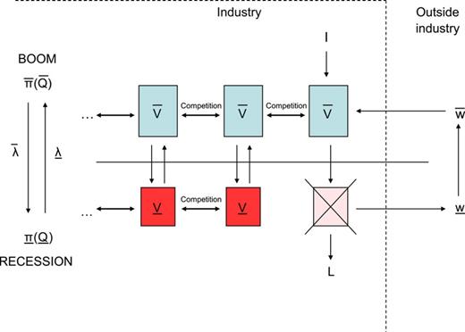
Industry dynamics. $\overline{V}$ and $\underset{¯}{V}$ denote the firm value in booms and recessions, respectively, I is the physical investment cost, L is the liquidation value, $\overline{w}$ and $\underset{¯}{w}$ (⁠$\overline{\pi }\left(\overline{Q}\right)$ and $\underset{¯}{\pi }\left(\underset{¯}{Q}\right)$⁠) represent outside wages (profits) in booms and recessions, respectively, and $\overline{\lambda }$ (⁠$\underset{¯}{\lambda }$⁠) denotes the hazard rate associated with the arrival of a recession (boom).

3.1 SOME BUILDING BLOCKS FOR VALUING CLAIMS

Before we solve for the owner–managers’ investment policy in industry equilibrium, we introduce the following proposition that provides the main building blocks for our future valuation problems (proofs are given in the Appendix).

Proposition 2.(a) The value of a claim that pays 1 dollar the first time when the economy switches from a boom (recession) to a recession (boom) equals$\overline{\delta }\equiv \frac{\overline{\lambda }}{r+\overline{\lambda }}$$\left(\underset{¯}{\delta }\equiv \frac{\underset{¯}{\lambda }}{r+\underset{¯}{\lambda }}\right)$

(b) The value of a claim that pays a cash-flow rate$\overline{\pi }$ ($\underset{¯}{\pi }$) for as long as the current boom (recession) lasts, and nothing thereafter, equals$\frac{\overline{\pi }}{r+\overline{\lambda }}$$\left(\frac{\underset{¯}{\pi }}{r+\underset{¯}{\lambda }}\right)$

(c) The value of a perpetual claim that pays a cash flow$\overline{\pi }$ during booms and$\underset{¯}{\pi }$ during recessions equals:

$$\begin{array}{l}{\overline{V}}_s(\overline{Q},\underset{¯}{Q})\equiv \frac{\overline{\pi }\left(\overline{Q}\right)}{r}(1-\overline{p})+\frac{\underset{¯}{\pi }\left(\underset{¯}{Q}\right)}{r}\overline{p}\text{\hspace{1em}when currently in a boom,}{\underset{¯}{V}}_s(\overline{Q},\underset{¯}{Q})\equiv \frac{\underset{¯}{\pi }\left(\underset{¯}{Q}\right)}{r}(1-\underset{¯}{p})+\frac{\overline{\pi }\left(\overline{Q}\right)}{r}\underset{¯}{p}\text{\hspace{1em}when currently in a recession,}\end{array}$$

(7)

where$\overline{p}\equiv \frac{\overline{\lambda }}{r+\overline{\lambda }+\underset{¯}{\lambda }}$ and$\underset{¯}{p}\equiv \frac{\underset{¯}{\lambda }}{r+\overline{\lambda }+\underset{¯}{\lambda }}$

The valuation formulas for ${\overline{V}}_s$ and ${\underset{¯}{V}}_s$ have simple intuitive interpretations. For example, ${\overline{V}}_s$ is a weighted average of the perpetuities $\frac{\overline{\pi }}{r}$ and $\frac{\underset{¯}{\pi }}{r}$⁠, where the former (latter) perpetuity denotes the present value of receiving the cash flow $\overline{\pi }$ (⁠$\underset{¯}{\pi }$⁠) forever.16 The weights are given by (⁠$1-\overline{p}$⁠) and $\overline{p}$⁠, where $0\le \overline{p}=\frac{\overline{\lambda }}{r+\overline{\lambda }+\underset{¯}{\lambda }}\le 1$⁠. If the likelihood of a switch to a recession is zero (⁠$\overline{\lambda }=0$ and hence $\overline{p}=0$⁠), then ${\overline{V}}_s$ simply equals $\frac{\overline{\pi }}{r}$ . As the hazard of switching from a boom to a recession becomes extremely large compared to the hazard of switching from a recession to a boom, the claim value ${\overline{V}}_s$ converges to $\frac{\underset{¯}{\pi }}{r}$⁠.

3.2 FIRST-BEST INVESTMENT POLICY

We now study entry and exit decisions in a competitive industry where each firm is run by an owner–manager who provides both the required physical capital (I) and the human capital (H). This benchmark case assumes that managers are not wealth constrained. Consequently, debt has no role to play.

The opportunity cost to each investor of not investing in human capital is the opportunity wage rate that could be earned outside the industry. Should a potential owner–manager decide never to invest then statement (c) in Proposition 2 implies that the value of her claim in booms, $\overline{W}$⁠, and in recessions, $\underset{¯}{W}$⁠, is given respectively by

$$\overline{W}=\frac{\overline{w}}{r}(1-\overline{p})+\frac{\underset{¯}{w}}{r}\overline{p}\text{\hspace{1em}and\hspace{1em}}\underset{¯}{W}=\frac{\underset{¯}{w}}{r}(1-\underset{¯}{p})+\frac{\overline{w}}{r}\underset{¯}{p}.$$

Consider next an owner–manager who operates in the industry during booms but leaves the industry during recessions. This type of owner–manager incurs a one-off investment cost H in human capital. She pays I at the start of each boom and receives cash flows at a rate $\overline{\pi }$ during each boom. She also receives the liquidation value L at the start of each recession and her opportunity wage rate $\underset{¯}{w}$ during recessions. Finally, an owner–manager who operates in the industry during booms and recessions incurs a one-off investment cost H and I at the start of the first boom and receives cash flows $\overline{\pi }$ (in booms) and $\underset{¯}{\pi }$ (in recessions) thereafter.

We focus in this paper on the case in which some firms leave in recession.17 We therefore impose the following condition throughout the paper (the derivation of this condition is given in the proof of Proposition 3):

Assumption 2. Demand shocks are sufficiently high such that some firms leave in recession, i.e.:,

$$\overline{\pi }\left(\tilde{Q}\right)-\underset{¯}{\pi }\left(\tilde{Q}\right)>(I-L)(r+\overline{\lambda }+\underset{¯}{\lambda })+\overline{w}+\frac{rH}{1-\overline{p}}-\underset{¯}{w},$$

(8)

where$\tilde{Q}$ is the solution to${\overline{V}}_s(\tilde{Q},\tilde{Q})=I+H+\overline{W}$.

How big demand shocks have to be depends on the other model parameters, such as the sunk cost of investment in human (H) and physical (I − L) capital. Higher sunk costs discourage exit and therefore need to be accompanied by relatively higher demand shocks for exit to occur. One can show, for example, that there exists a critical threshold $\tilde{H}$ such that exit occurs for $H<\tilde{H}$ and no exit occurs for $H\ge \tilde{H}$ (holding all else constant). One can prove (see Appendix) the following proposition:

Proposition 3.The first-best industry output in booms ($\overline{Q}$) and recessions ($\underset{¯}{Q}$) are the solution to the following equations:

$$\overline{\pi }\left(\overline{Q}\right)=[rI+\overline{\lambda }(I-L\left)\right]+\left[\overline{w}+\frac{rH}{1-\overline{p}}\right]\equiv {\overline{\pi }}^o\left(L\right)=\text{charge\hspace{0.17em}for\hspace{0.17em}physical\hspace{0.17em}capital}+\text{charge\hspace{0.17em}for\hspace{0.17em}human\hspace{0.17em}capital,}$$

(9)

$$\underset{¯}{\pi }\left(\underset{¯}{Q}\right)=[rL-\underset{¯}{\lambda }(I-L\left)\right]+\underset{¯}{w}\equiv {\underset{¯}{\pi }}^o\left(L\right)=\text{charge\hspace{0.17em}for\hspace{0.17em}physical\hspace{0.17em}capital}+\text{charge\hspace{0.17em}for\hspace{0.17em}human\hspace{0.17em}capital.}$$

(10)

The value of survivors and leavers in respectively booms and recessions are

$${\overline{V}}_{\text{s}}(\overline{Q},\underset{¯}{Q})={\overline{V}}_{\text{l}}(\overline{Q},\underset{¯}{Q})=I+H+\overline{W}\text{\hspace{1em}and\hspace{1em}}{\underset{¯}{V}}_{\text{s}}(\overline{Q},\underset{¯}{Q})=L+\underset{¯}{W}+\underset{¯}{\delta }H,$$

(11)

where the subscripts “l” and “s” refer to firms that leave and survive in recession, respectively.

The proposition gives simple intuitive expressions for the equilibrium profit rates in booms and recessions. The equilibrium profits can be decomposed in a charge for physical capital and a charge for human capital (the result parallels the scenario with a competitive labor market in Baldwin, 1983). During booms, the charge for physical capital equals the opportunity cost of the capital invested (rI) plus a risk premium for the hazard of recession (⁠$\overline{\lambda }(I-L)$⁠). Conversely, during recessions, the charge for physical capital equals the opportunity cost of liquidating the firm (rL) minus a discount for the hazard of economic recovery.

During booms the charge for human capital consists of the opportunity wage $\overline{w}$ plus a charge equal to $\frac{rH}{1-\overline{p}}=rH\left(1+\frac{\overline{\lambda }}{r+\underset{¯}{\lambda }}\right)$ for the investment in human capital. In the limiting case, where the industry stays in a boom forever (⁠$\overline{\lambda }=0$⁠), the required rate of return on H is just the risk-free rate r. If the hazard rate of switching from a boom to a recession is strictly positive (⁠$\overline{\lambda }>0$⁠), then the required rate of return increases by $\frac{\overline{\lambda }r}{r+\underset{¯}{\lambda }}$⁠, which reflects the discounted value of forgoing rH during recession $\left(\frac{rH}{r+\underset{¯}{\lambda }}\right)$ times the hazard rate of a recession arriving (⁠$\overline{\lambda }$⁠) when the economy is in a boom. Since managers that lose their job in recession merely earn the opportunity wage $\underset{¯}{w}$⁠, the longer (shorter) recessions (booms) are expected to last, the larger profits have to be during booms to recover the investment in human capital. Consider the limiting case where a recession is expected to last forever (⁠$\underset{¯}{\lambda }=0$⁠), once arrived. In that case, human capital becomes useless for those managers that leave the industry, and as a result the required rate of return on human capital becomes $H(r+\overline{\lambda })$⁠: the interest rate r is simply augmented by $\overline{\lambda }$⁠, where $\overline{\lambda }$ can now be interpreted as a risk of “ruin.”

Unlike physical capital, human capital cannot be traded. Consequently, it cannot be liquidated in recession. Instead, it temporarily leaves the industry and returns in booms. This difference explains the asymmetry in the expressions for the charge for human and physical capital.

3.3 EXTENSIONS AND GENERALIZATIONS

Our model assumes that managers incur the investment cost in human capital, H, only once. It is possible to generalize the model to the case where managers active in the industry have to incur the cost H at future random arrival times if they wish to retain their job.18 The need to make additional investment in human capital could result from drastic changes or innovations within the industry that require managers to retrain or incur costs of adjustment.

When the industry is in a boom (recession), an additional cost H has to be incurred according to a Poisson arrival process with parameter $\overline{\gamma }$ (⁠$\underset{¯}{\gamma }$⁠). Assume that the Poisson processes for $\overline{\lambda }$⁠, $\underset{¯}{\lambda }$⁠, $\overline{\gamma }$⁠, and $\underset{¯}{\gamma }$ are independent.

If $\underset{¯}{\gamma }>0$⁠, then the industry output can take on three different values over time, which we denote by $\overline{Q}$⁠, $\underset{¯}{Q}$⁠, and $\widehat{\underset{¯}{Q}}$⁠. At the start of a boom, all managers entering the industry for the first time pay H and are aware that further investments in human capital may be required. When subsequently additional investment during a boom is required, managers are in the same situation as when they initially entered (bear in mind that the initial investment H is now sunk and irrelevant in managers’ decision making): they are required to pay H, knowing additional subsequent investments in human capital may be required. In booms, managers will therefore always decide in favor of making the additional investment H. Of course, the higher the likelihood of subsequent investments, the fewer managers enter the industry in the first place. Therefore, the industry output in booms, $\overline{Q}$⁠, is inversely related to $\overline{\gamma }$ (and $\underset{¯}{\gamma }$⁠).

When a recession arrives, firms leave the industry until the marginal firm is indifferent between staying or leaving. The resulting industry output at the start of the recession is $\underset{¯}{Q}$ (⁠$<\overline{Q}$⁠). Managers that remain active in the industry are aware that future investment in human capital may be required during recession. If an additional cost H actually needs to be incurred before the economy reverts to a boom, then some firms leave the industry causing the output to drop to $\widehat{\underset{¯}{Q}}$ (⁠$<\underset{¯}{Q}$⁠). As a result, industry exit can be “staggered”: a first wave of departures occurs at the start of the recession, and a second wave of closures happens the first time when further investment in human capital is required during a recession. Note that further investments in human capital during recession (but after the second closure wave) do not induce any further exit for the same reason why additional investments in human capital during booms do not lead to departures.

Although conceptually the solutions for $\overline{Q}$⁠, $\underset{¯}{Q}$⁠, and $\widehat{\underset{¯}{Q}}$ can be derived analogously as before, the expressions for the corresponding firm values (⁠$\overline{V}$⁠, $\underset{¯}{V}$⁠, and $\widehat{\underset{¯}{V}}$⁠) become much more elaborate. In the interest of space, we do not report them in the paper.19

4. The Dynamic Model with Separation of Equity and Human Capital

We now introduce separation between ownership of human capital and equity capital. As was shown in Section 2, debt now acts as a balancing variable between equityholders and managers. The following assumption formalizes the concept of “net debt” and specifies the priority structure at closure among the firm’s stakeholders:

Assumption 3.The firm’s net debt, D, is defined as the difference between the firm’s debt liabilities and its liquid assets. The firm pays (receives) a coupon flow rD for positive (negative) D until the firm is closed.20If net debt is negative (D < 0), then equityholders receive upon closure L plus the liquid assets −D (i.e., L − D). If net debt is positive, then bondholders have a first claim (up to D) on the assets L in liquidation, with equityholders having the entire residual claim (L − D)⁺. If the firm defaults on its debt obligations (D > L), then bankruptcy costs amount toϕL.

If D is positive, then the firm’s net debt position is equivalent to a standard perpetual debt contract with coupon rD that is terminated when the firm defaults. We assume that the debt is secured by the firm’s physical assets, which means that at closure bondholders receive min{D, L(1 − ϕξ)} (with ξ = 1 if D > L, and ξ = 0 otherwise), whereas equityholders receive (L − D)⁺. This payoff follows from the fact that upon default bondholders liquidate the firm (like equityholders, bondholders are unable to run the firm as a going concern). Equityholders default on the debt contract if D > L. Bankruptcy costs associated with default are a fraction ϕ of the liquidation value L and reduce bondholders’ payoff. Bankruptcy costs do not represent the difference between investment cost and the resale value of assets per se but reflect the deadweight cost of the transfer of ownership from original equityholders to creditors.21

The firm needs both physical capital (owned by shareholders) and human capital (owned by wealth constrained managers) to be operational.22 No cash flows are generated while either party abstains. It is this mutual cost of a stalemate that forces both parties to negotiate an agreement to share the free cash flows.

When economic conditions deteriorate and free cash flows plummet, it may no longer be optimal for equityholders and managers to stay together within the firm. Each party can permanently abandon the firm: equityholders can liquidate the physical assets, whereas managers can resign to receive their outside reservation wage. While managers cannot liquidate their human capital, they can re-enter the industry at some future point without having to incur the investment in human capital again. Managers’ option to leave the industry in recession therefore embeds an option to return in booms.

We adopt the standard assumption that the cash flows generated by the firm are observable but nonverifiable.23 In this paper, we therefore do not derive explicit contracts but self-enforcing agreements and remuneration that, at each moment in time, are the outcome of bargaining between the equityholders and the managers (also known as “implicit contracts”).24

We now need to decide on a bargaining model to determine how free cash flows are shared between equityholders and managers. The main bargaining models used in the finance literature are: the Nash (1950) bargaining model and the Rubinstein (1982) bargaining model (and their variations). In the Rubinstein game, the alternative opportunity is modeled as an “outside option” where a party must quit the bargaining table permanently in order to take up the alternative opportunity. For example, the manager must permanently resign in order to take up a post elsewhere. In the Nash-bargaining game, the alternative opportunity is modeled as a “threat point.” The underlying assumption is that a party can collect its threat point payoffs for as long as a bargaining agreement has not been reached. For example, the manager takes up a temporary post elsewhere while bargaining takes place.25

The difference between an outside option and a threat point results in a different bargaining solution. While in the Nash bargaining solution each party’s share is strictly increasing in the value of its threat point, in the Rubinstein bargaining solution each party gets the best (i.e., the maximum) of its outside option and the bargaining share that it would obtain in the absence of outside options. The outside option thus acts as a lower bound or “constraint” on the equilibrium share.

Since equityholders’ decision to liquidate and managers’ decision to resign are permanent and irreversible, we have a two player game between equityholders and managers where each party has an outside option. The value of this outside option in booms (recessions) is denoted by ${\overline{o}}_{\text{e}}$ and ${\overline{o}}_{\text{m}}$ (⁠${\underset{¯}{o}}_{\text{e}}$ and ${\underset{¯}{o}}_{\text{m}}$⁠) for equityholders and managers, respectively. We focus on the limiting case where the bargaining interval goes to zero and bargaining can take place continuously. As such, our game is a continuous-time variation of the Shaked and Sutton (1984) and Binmore, Rubinstein, and Wolinsky (1986) models of bargaining with outside options and risk of breakdown during negotiation.26 Its solution is a fairly standard result in the bargaining literature and given below.27

Result 1.During booms the compensation rate for human capital ($\overline{s}$) and the payout rate to equityholders ($\overline{d}$) both equal one half of the free cash flows:$\overline{s}=\overline{d}=\frac{\overline{\pi }-rD}{2}$. During recessions, the compensation and payout rate are such that equityholders’ and managers’ outside option exactly bind (i.e.,$\underset{¯}{E}={\underset{¯}{o}}_{\text{e}}$ and$\underset{¯}{M}={\underset{¯}{o}}_{\text{m}}$).

During booms, equityholders and the providers of human capital each get half of the profits after interest repayments if net debt is positive (D ≥ 0) or half of the combined value of operating profits and the interest generated by liquid assets if net debt is negative (D < 0). This property is valid irrespective of whether any outside options bind in recession or whether the debt is risky. This does, however, not mean that the payout to equityholders and managers in booms is independent of what happens in recession or of how much each party invests. We show below that the equilibrium profits $\overline{\pi }$ and the optimal debt level D are very much influenced by the other model parameters.

In equilibrium, free cash flows are equally shared in booms (i.e., η = 0.5) because outside options do not bind in booms and both parties are otherwise symmetric (e.g., they have the same discount rate). Equal sharing is under those circumstances a standard feature of Rubinstein style bargaining models.28 Importantly, the results that follow do not depend in any fundamental way on the shares being exactly equal. As was shown in Section 2, our model and its results can easily be generalized to the case where $\overline{s}=\eta (\overline{\pi }-rD)$ and $\overline{d}=(1-\eta )(\overline{\pi }-rD)$ with $0<\eta <1$⁠.

In recession, each party’s claim value equals exactly its outside option value because when the economy switches from a boom to a recession firms keep leaving up to the point where equityholders and managers are indifferent between staying or leaving.29

Proposition 2 and Result 1 together imply that the equityholders’ and managers’ claim values are given by

$$\begin{array}{l}\overline{E}=\frac{\overline{\pi }-rD}{2(r+\overline{\lambda })}+\overline{\delta }\underset{¯}{E}\text{\hspace{1em}and\hspace{1em}}\underset{¯}{E}={\underset{¯}{o}}_{\text{e}},\\ \overline{M}=\frac{\overline{\pi }-rD}{2(r+\overline{\lambda })}+\overline{\delta }\underset{¯}{M}\text{\hspace{1em}and\hspace{1em}}\underset{¯}{M}={\underset{¯}{o}}_{\text{m}}.\end{array}$$

The above equations determine the equityholders’ and managers’ claim for exogenously given profit levels, debt principal, and outside option values. We now endogenize the values of these entities. The following proposition states the value of a firm’s outside options as a function of its debt principal.

Proposition 4.In recessions, the value of equityholders’ outside option (${\underset{¯}{o}}_{\text{e}}$) and of managers’ outside option (${\underset{¯}{o}}_{\text{m}}$) are given respectively by

$$\begin{array}{l}{\underset{¯}{o}}_e={(L-D)}^{+},\\ {\underset{¯}{o}}_m=\frac{\underset{¯}{w}}{r}(1-\underset{¯}{p})+\frac{\left[\right(r+\overline{\lambda })I-\overline{\lambda }L(1-\varphi \xi )-rD]}{r}\underset{¯}{p}.\end{array}$$

It follows immediately from equityholders’ limited liability that their payoff from leaving the firm in recession is given by ${\underset{¯}{o}}_{\text{e}}={(L-D)}^{+}$⁠. The value of managers’ outside option in recession, ${\underset{¯}{o}}_{\text{m}}$⁠, equals the present value of the wage rate $\underset{¯}{w}$ that managers get when they leave the industry during recession and the salary rate they receive when returning to the industry during booms. Note that ${\underset{¯}{o}}_{\text{m}}$ depends on the leavers’ debt level because managers’ option to leave the industry in recession includes an option to return in booms. Consequently, the debt level that new entrants subsequently adopt in booms determines managers’ future salary.

Armed with our expressions for ${\underset{¯}{o}}_{\text{e}}$ and ${\underset{¯}{o}}_{\text{m}}$⁠, we can now solve for the industry equilibrium. We first derive the claim value of those firms that, in equilibrium, leave the market. To do so, we need to pin down the following three unknowns: $\overline{\pi }$⁠, ${\overline{s}}_{\text{l}}$⁠, and $D_{\text{l}}$ (remember that managers leave the industry during recession and therefore ${\underset{¯}{s}}_{\text{l}}=\underset{¯}{w}$⁠). ${\overline{s}}_{\text{l}}$ is determined by the bargaining solution (i) ${\overline{s}}_{\text{l}}=\frac{\overline{\pi }-r{D}_{\text{l}}}{2}$⁠. Equity capital is supplied competitively, causing equityholders to break even upon investment, i.e., (ii) ${\overline{E}}_{\text{l}}=I-{\overline{B}}_{\text{l}}$⁠, where B generally denotes the market value of debt. This gives an equilibrium condition for $\overline{\pi }$⁠. Finally, we need to determine the debt principal D_l of firms that leave the industry. Assuming without loss of generality that equityholders set debt policy then they choose the firm’s debt principal D_l (or coupon level rD_l) so as to maximize their payoff at investment, subject to the managers’ participation constraint.30 Or, equivalently, D_l is the solution to the following constrained maximization problem:

$$\underset{D_{\text{l}}}{\text{max}}\{{\overline{E}}_{\text{l}}-(I-{\overline{B}}_{\text{l}}\left)\right\}\text{\hspace{1em}subject\hspace{0.17em}to\hspace{0.17em}}{\overline{M}}_{\text{l}}\ge \overline{W}+H.$$

(12)

A higher debt level unambiguously lowers managers’ claim because debt reduces free cash flows and therefore managers’ salary rate ${\overline{s}}_{\text{l}}=\frac{\overline{\pi }-r{D}_{\text{l}}}{2}$ (note that an atomistic firm cannot influence $\overline{\pi }$ through its debt policy). On the other hand, a higher debt level increases equityholders’ payoff from investment. For every dollar of debt raised, equityholders have to contribute one dollar less to the investment, but they share the pain of the subsequent interest repayment with managers (since ${\overline{d}}_{\text{l}}={\overline{s}}_{\text{l}}$⁠).

If equityholders’ payoff were everywhere monotonically increasing in the debt principal, then equityholders would raise debt up to the point where managers’ participation constraint becomes binding, and D_l would simply be pinned down by condition (iii) ${\overline{M}}_{\text{l}}=\overline{W}+H$⁠. We show, however, in the Appendix that equityholders’ payoff ${\overline{E}}_{\text{l}}-(I-{\overline{B}}_{\text{l}})$ is monotonically increasing in D_l, except at D_l = L, where there can be a discrete downward jump if bankruptcy costs are strictly positive. At D_l = L, a marginal increase in the debt level leads to a discrete fall in the market value of the debt, ${\overline{B}}_{\text{l}}$⁠, because of the deadweight cost of bankruptcy. Depending on the value of H, this leads to three possible regimes for the optimal debt level:

1. For sufficiently high levels of H (i.e., $H^{\text{*}}<H$⁠, where $H^{\text{*}}$ is defined below), D_l is the solution to (iii) ${\overline{M}}_{\text{l}}=\overline{W}+H$ and managers’ participation constraint binds at a level D_l < L.

2. For sufficiently low levels of H (i.e., $H<H^{\text{**}}$⁠, where $H^{\text{**}}$ is defined below), D_l is again the solution to (iii) ${\overline{M}}_{\text{l}}=\overline{W}+H$ but the debt level D_l for which managers’ participation constraint binds exceeds L, i.e., D_l > L.

3. For an intermediate region (i.e., $H^{\text{**}}\le H\le H^{\text{*}}$⁠), a risky debt level (D > L) could be adopted while still ensuring managers’ participation. However, the gain from constraining managers is wiped out by the deadweight costs of bankruptcy, which reduce the proceeds from the debt issue in a discrete fashion. The debt level is therefore restricted to (iii) D_l = L. By constraining debt to the firm’s liquidation value, managers’ participation constraint is no longer binding (i.e., ${\overline{M}}_{\text{l}}>\overline{W}+H$⁠). Only when H is below $H^{\text{**}}$ does it pay off to issue risky debt and to raise the principal by a discrete amount over and beyond L.

Why can managers enjoy excess rents (⁠${\overline{M}}_{\text{l}}>\overline{W}+H$⁠), whereas equityholders cannot? Managers cannot commit to taking less than ${\overline{s}}_{\text{l}}$ of the free cash flows. Given that managers’ claim cannot be traded in financial markets (unlike equity), it is not possible for investors to compete away excess value. Managers can neither compete away among themselves the excess value because this would require that they coinvest an amount equal to the present value of their excess rents when joining the firm. Wealth constraints prevent managers from doing this.

We now sketch the derivation of the claim values of those firms that do not leave in recession (“stayers”). To identify the claim values, we need to solve for four unknowns: $\underset{¯}{\pi }$⁠, ${\overline{s}}_{\text{s}}$⁠, ${\underset{¯}{s}}_{\text{s}}$⁠, and D_s. Competitive exit ensures that firms leave up to the point where both parties’ outside options are binding in recession (i.e., managers and equityholders are indifferent between staying or leaving in recession): (i) ${\underset{¯}{E}}_{\text{s}}={\underset{¯}{o}}_{\text{e}}$⁠, and (ii) ${\underset{¯}{M}}_{\text{s}}={\underset{¯}{o}}_{\text{m}}$⁠.31 The bargaining solution for booms implies that (iii) $\frac{\overline{\pi }-r{D}_s}{2}$⁠. Finally, (iv) ${\overline{E}}_{\text{s}}=I-D_{\text{s}}$ because outside equity is supplied on a competitive basis.32 Conditions (i), (ii) (iii), and (iv) determine $\underset{¯}{\pi }$⁠, ${\underset{¯}{s}}_{\text{s}}$⁠, ${\overline{s}}_{\text{s}}$⁠, and $D_{\text{s}}$⁠.33

Our analysis assumes that equityholders set the debt level. Would the results be different if managers were to set the debt level? The answer is no. In equilibrium, equityholders’ participation constraint is always binding in a competitive equity market. Equityholders’ claim increases in the debt level. As a result, it is not possible for managers to reduce the debt any further without violating equityholders’ participation constraint. The same debt level is therefore also constrained optimal from managers’ viewpoint.

In what follows Propositions 5–7 state and discuss the industry equilibrium for different levels H of investment in human capital. The solution naturally splits up in three cases: high (⁠$H^{\text{*}}\le H$⁠), intermediate (⁠$H^{\text{**}}\le H\le H^{\text{*}}$⁠), and low (⁠$H<H^{\text{**}}$⁠) levels of human capital.

Proposition 5.If firms are highly human capital intensive (i.e., if the investment H in human capital satisfies $H^{\text{*}}<H$⁠), then we observe “regime 1” in which all firms adopt the same risk-free debt level and some firms leave in recession. The debt, firm profits and managerial compensation are given by

$$D_1\left(L\right)=D_{1\text{s}}\left(L\right)=D_{1\text{l}}\left(L\right)=I+\frac{\overline{\lambda }}{r}(I-L)-\frac{\overline{w}}{r}-\frac{H}{1-\overline{p}}=L-\frac{(H-H^{\text{*}})}{1-\overline{p}},$$

$${\overline{\pi }}_1\left(L\right)=rI+\overline{\lambda }(I-L)+\overline{w}+\frac{rH}{1-\overline{p}}={\overline{\pi }}^{\text{o}}\left(L\right),$$

$${\underset{¯}{\pi }}_1\left(L\right)=rL-\underset{¯}{\lambda }(I-L)+\underset{¯}{w}={\underset{¯}{\pi }}^{\text{o}}\left(L\right),$$

$${\overline{s}}_{\text{1s}}={\overline{s}}_{\text{1l}}=\overline{w}+\frac{rH}{1-\overline{p}}\text{\hspace{1em}and\hspace{1em}}{\underset{¯}{s}}_{\text{1s}}={\underset{¯}{s}}_{1\text{l}}=\underset{¯}{w},$$

where $H^{\text{*}}$ is the solution to

$$\overline{w}+\frac{r{H}^{\text{*}}}{1-\overline{p}}=(I-L)(r+\overline{\lambda }).$$

(13)

Proposition 5 gives the optimal investment and debt policy when the investment in human capital H is relatively large (i.e., $H^{\text{*}}<H$⁠). We find that all firms adopt the same safe debt level (i.e., $D_{\text{s}}=D_{\text{l}}\equiv D^{\text{o}}<L$⁠). The optimal debt level has a very simple interpretation. It is the debt level that sets equityholders’ (leverage adjusted) payout rate in booms equal to managers’ salary rate, i.e.: ${\overline{d}}^{\text{o}}\equiv r(I-D^{\text{o}})+\overline{\lambda }(I-L)=\overline{w}+\frac{rH}{1-\overline{p}}\equiv {\overline{s}}^{\text{o}}\left(H\right)$⁠. Therefore, unlike in Dasgupta and Sengupta (1993), safe debt plays a meaningful role. The relation between the level of debt and market uncertainty depends on the relative magnitudes of I − L and H. If physical capital is more irreversible (large I − L), D increases with uncertainty. In the opposite case (i.e., large H), the relationship between debt and uncertainty is negative (as in Berk, Stanton, and Zechner, 2010). Finally, managers (equityholders) receive the efficient salary (payout) rate at all times.34

The equilibrium is identical to the first-best solution in Section 3 where there is no separation between equityholders and managers. Full efficiency is achieved thanks to competition and an optimal debt policy that ensures that equityholders and managers each get a fair return on their investment. If a firm requires more investment in human capital, then, all else equal, the level of debt in equilibrium is lower. For sufficiently high levels of investment in human capital, net debt gets negative. In particular, negative debt occurs if the sunk investment in human capital (H) and the opportunity cost of human capital (⁠$\overline{w}$⁠) are sufficiently large compared to the sunk cost (I − L) and the cost (I) of physical capital. Our result is therefore related to that of Perotti and Spier (1993). In their paper, underinvestment could be eliminated by issuing a strictly positive amount of debt. In our model, the optimal choice of leverage leads to efficient investment as well. Still, this optimal choice may be associated with negative net debt. The optimal debt level is decreasing in the firm’s liquidation value. This last result may come as a surprise as it implies that leverage is negatively related to tangibility, which is inconsistent, for example, with the trade-off theory of capital structure. Since debt is overcollateralized (D < L) bankruptcy costs are, however, not an issue. Higher tangibility means simply that equityholders get more of their capital investment back upon closure and, as a result, are willing to accept a lower debt level.35 We show below that this negative relation between tangibility and leverage is reversed when firms constrain their debt level because of bankruptcy cost considerations.

Before formulating the results for regime 2, we make the following assumption:

Assumption 4.Bankruptcy costs are not excessively high, that is,ϕ <ϕ*, whereϕ* is the root to:${\overline{\pi }}^{-1}[rI+(I-L\left)\right(r+2\overline{\lambda }\left)\right]={\underset{¯}{\pi }}^{-1}\left[{\underset{¯}{\pi }}^o-\frac{\overline{\lambda }\underset{¯}{\lambda }{\varphi }^{\text{*}}L}{r+\overline{\lambda }}\right]$.

Now, we are ready to describe the solution for regime 2, which prevails for intermediate levels of human capital (i.e., $H\in [H^{\text{**}},H^{\text{*}}]$⁠).

Proposition 6.If the investment H in human capital satisfies$H^{\text{**}}\le H<H^{\text{*}}$, then we observe“regime 2” in which all firms adopt the same risk-free debt level L and some firms leave in recession. The debt, firm profits, and managerial compensation are given by

$$\begin{array}{l}{D}_2\left(L\right)=D_{2\text{s}}\left(L\right)=D_{2\text{l}}\left(L\right)=L,\\ {\overline{\pi }}_2\left(L\right)=rI+(r+2\overline{\lambda })(I-L)>{\overline{\pi }}^{\text{o}}\left(L\right)\text{\hspace{1em}and\hspace{1em}}{\underset{¯}{\pi }}_2\left(L\right)=rL-\underset{¯}{\lambda }(I-L)+\underset{¯}{w}={\underset{¯}{\pi }}^{\text{o}}\left(L\right),\\ {\overline{s}}_{\text{2s}}\left(L\right)={\overline{s}}_{2\text{l}}\left(L\right)=(r+\overline{\lambda })(I-L)\text{\hspace{1em}and\hspace{1em}}{\underset{¯}{s}}_{2\text{s}}={\underset{¯}{s}}_{2\text{l}}=\underset{¯}{w},\end{array}$$

where $H^{\text{**}}$ is the solution to

$$\overline{w}+\frac{r{H}^{\text{**}}}{1-\overline{p}}=(I-L)(r+\overline{\lambda })-\overline{\lambda }\varphi L.$$

(14)

Regime 2 only occurs if bankruptcy costs are strictly positive (i.e.,$H^{\text{**}}<H^{\text{*}}\iff \mathrm{\varphi }>0$⁠).

Regime 2 arises for intermediate levels of human capital (i.e., if $H^{\text{**}}\le H<H^{\text{*}}$⁠). The optimal debt policy for all firms is to adopt a debt level D_s = D_l = L. By constraining the debt level to L, managers’ investment in human capital has a strictly positive NPV (i.e., ${\overline{M}}_{\text{s}}={\overline{M}}_{\text{l}}>\overline{W}+H$⁠). Bankruptcy costs make it, however, not optimal to raise debt levels. Equityholders break even in booms and recessions. Since D = L, equity has a zero (or arbitrarily small) value in recessions. Managers’ salary rate exceeds the efficient compensation rate during booms and equals the outside wage rate during recessions. As higher bankruptcy costs are associated with a wider range of parameter values for which region 2 prevails, wages on average increase with bankruptcy costs.36 Equityholders payout rate equals the efficient rate at all times. The total profit rate in booms exceeds the first-best profit rate (⁠$\overline{\pi }>{\overline{\pi }}^{\text{o}}$⁠), which implies that there is insufficient entry in booms (entry is insufficient as long as $\varphi >0$⁠). The industry output level is, however, efficient in recessions.

Proposition 7 presents the solution for low levels of human capital (i.e., $H<H^{\text{**}}$⁠).

Proposition 7.If$H<H^{\text{**}}$, then we observe “regime 3” in which some firms adopt a high debt level and some firms adopt a lower debt level. The former firms leave the industry in recession. The debt value exceeds L for all firms. The debt, profits, and managerial compensation are given by

$$D_{3\text{l}}\left(L\right)=I+\frac{\overline{\lambda }}{r}(I-L)+\frac{\overline{\lambda }}{r}\varphi L-\frac{\overline{w}}{r}-\frac{H}{1-\overline{p}}=L+\frac{(H^{\text{**}}-H)}{1-\overline{p}}+2\frac{\overline{\lambda }}{r}\varphi L,$$

$$D_{3\text{s}}\left(L\right)=\frac{1}{r+2\overline{\lambda }}\left[(r+\overline{\lambda })I+\overline{\lambda }L(1-\varphi )-\overline{w}-\frac{rH}{1-\overline{p}}\right]=L+\frac{r(H^{\text{**}}-H)}{(r+2\overline{\lambda })(1-\overline{p})},$$

$${\overline{\pi }}_3\left(L\right)=rI+\overline{\lambda }(I-L)+\overline{\lambda }\varphi L+\overline{w}+\frac{rH}{1-\overline{p}}>{\overline{\pi }}^{\text{o}}\left(L\right),$$

$${\underset{¯}{\pi }}_3\left(L\right)=r{D}_{3\text{s}}-\underset{¯}{\lambda }(I-D_{3\text{s}})+{\underset{¯}{s}}_{3\text{s}}={\underset{¯}{\pi }}^{\text{o}}\left(L\right)+\frac{r^2(H^{\text{**}}-H)(r+\overline{\lambda }+\underset{¯}{\lambda })}{(r+2\overline{\lambda })(1-\overline{p})(r+\overline{\lambda })}-\frac{\overline{\lambda }\underset{¯}{\lambda }\varphi L}{r+\overline{\lambda }},$$

$${\overline{s}}_{3\text{l}}=\overline{w}+\frac{rH}{1-\overline{p}}\text{\hspace{1em}and\hspace{1em}}{\underset{¯}{s}}_{3\text{l}}=\underset{¯}{w},$$

$${\overline{s}}_{3\text{s}}\left(L\right)=\frac{r+\overline{\lambda }}{r+2\overline{\lambda }}\left[\overline{w}+\frac{rH}{1-\overline{p}}+\overline{\lambda }(I-L(1-\varphi \left)\right)\right]>{\overline{s}}_{3\text{l}},$$

$${\underset{¯}{s}}_{\text{3s}}\left(L\right)=\underset{¯}{w}-\frac{\underset{¯}{\lambda }}{r+\overline{\lambda }}({\overline{s}}_{3\text{s}}-{\overline{s}}_{\text{3l}})=\underset{¯}{w}-\frac{\overline{\lambda }\underset{¯}{\lambda }}{(r+\overline{\lambda })}\left[\frac{r(H^{\text{**}}-H)}{(r+2\overline{\lambda })(1-\overline{p})}+\varphi L\right].$$

Proposition 7 states that if the required investment in human capital is low (i.e., $H<H^{\text{**}}$⁠), then all firms adopt a debt level that exceeds L in order to constrain managers in booms. Furthermore, firms that leave in recession adopt a higher debt level than survivors. High leverage prevents managers from capturing excess rents in booms, but causes these firms to incur bankruptcy costs in recession. Survivors, on the other hand, set their debt level sufficiently low so that in recession equityholders and managers are indifferent between staying and leaving. By doing so, these firms are able to issue risk-free debt. However, by constraining the debt level, managers of these firms get excess rents in booms (i.e., ${\overline{s}}_{3\text{s}}>{\overline{s}}_{3\text{l}}$⁠).37 These excess rents are partially clawed back in recession when managers of the surviving firms get paid below their reservation wage. Managers are willing to accept this cut because of the prospect of superior rents in future booms.38 While managers of firms that leave in recession break even in booms and recessions, managers of firms that stay have a positive NPV claim in booms (i.e., ${\overline{M}}_{3\text{s}}>\overline{W}+H$⁠). This means that there is a first-mover advantage for managers that enter first into the industry and it explains why these managers do not leave in recession despite being paid below the reservation wage. First movers have an interest to adopt a low debt level because by doing so these firms capture upon investment a positive NPV equal to

$${\overline{E}}_{3\text{s}}+{\overline{M}}_{3\text{s}}+D_{3\text{s}}-I-\overline{W}-H={\overline{M}}_{3\text{s}}-\overline{W}-H>0.$$

Even though equityholders of all firms only break even, the market capitalization of first movers is larger (i.e., ${\overline{E}}_{3\text{s}}=I-D_{3\text{s}}>{\overline{E}}_{3\text{l}}=I-{\overline{B}}_{3\text{l}}$ since ${\overline{B}}_{3\text{l}}>D_{3\text{s}}$⁠).

Undercollateralized debt leads to inefficiencies because it brings with it bankruptcy costs and debt overhang. The highly levered firms anticipate future bankruptcy costs and therefore require a higher equilibrium profit rate in booms to compensate. This creates underinvestment in booms.39 Firms that plan to stay in recession constrain their debt level such that both managers’ and equityholders’ outside option exactly binds in recession. This lower debt level gives managers excess rents in booms (⁠${\overline{s}}_{3\text{s}}>{\overline{s}}_{3\text{l}}=\overline{w}$⁠). These excess rents increase with bankruptcy costs and allow managers’ compensation to be cut in recession below the reservation wage by an amount $\frac{\underset{¯}{\lambda }}{r+\overline{\lambda }}({\overline{s}}_{3\text{s}}-{\overline{s}}_{3\text{l}})$⁠. This provides space for profits to be reduced in recession by an equal amount. Bankruptcy costs therefore create an overinvestment effect in recession. On the other hand, the profit rate ${\underset{¯}{\pi }}_3$ increases to the extent that D exceeds L. Since equityholders have limited liability, undercollateralized debt leads to the well-known (Myers, 1977) underinvestment effect. To summarize, for values of H just below $H^{\text{**}}$⁠, the bankruptcy cost effect dominates, resulting in overinvestment (i.e., insufficient exit) during recession, whereas for lower levels of H, the debt level adopted is much higher and this causes the debt overhang effect to dominate in recession (i.e., too much exit).

Regime 3 is derived under the assumption that some firms leave in recession. However, as ϕ increases, the equilibrium profit rate in booms (recessions) unambiguously rises (falls) (see Proposition 7). Consequently, the industry output in booms (recessions) monotonically falls (rises) as ϕ increases. There exists therefore a level ${\varphi }^{\text{*}}$ for which $\overline{Q}$ equals $\underset{¯}{Q}$⁠, and firms no longer leave the market40: bankruptcy costs lower the firm’s liquidation value and, as such, lead to more hysteresis. For sufficiently high levels of bankruptcy costs, industry output therefore remains constant. Typical values for ${\varphi }^{\text{*}}$ are, however, unrealistically high from an economic viewpoint.41 We therefore do not discuss the case $\varphi >{\varphi }^{\text{*}}$⁠.42

Figure 2 illustrates and summarizes the paper’s main results.43 Panel A illustrates the negative relation between the debt principal, D, and the (sunk) cost of human capital investment, H. The debt principal is not a strictly decreasing function of H. The flat segment is due to the presence of bankruptcy costs. For H falling into the interval $[H^{\text{**}},H^{\text{*}}]=[39.06,53.12]$ firms adopt in equilibrium the second-best level of debt equal to L. Such a policy allows shareholders to avoid bankruptcy costs but is associated with excess rents for managers. For $H<H^{\text{**}}=39.06$⁠, the benefit of constraining managers dominates the expected bankruptcy costs: firms adopt risky debt that increases expected bankruptcy costs but allows for concessions from managers. Figure 2 confirms that for $H<H^{\text{**}}$ firms that are expected to leave the industry in recession (i.e., the second movers) adopt a risky debt level (D > L) that is substantially higher than their surviving counterparts (i.e., the first movers).

Figure 2

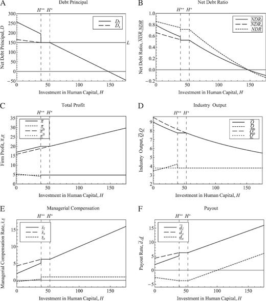
Comparative statics results for debt principal, NDR, total profit, industry output, managerial compensation, and payout to shareholders generated for the following parameter values: $\overline{\pi }\left(Q\right)=\overline{a}{Q}^{-\mathit{ϵ}}-\overline{b}$ and $\underset{¯}{\pi }\left(Q\right)=\underset{¯}{a}{Q}^{-\mathit{ϵ}}-\underset{¯}{b}$⁠, where $\overline{a}=200$⁠, $\underset{¯}{a}=25$⁠, $\overline{b}=\underset{¯}{b}=1$⁠, and $\mathit{ϵ}=1.1$⁠. Furthermore, $\overline{\lambda }=\underset{¯}{\lambda }=0.075$⁠, $r=0.05$⁠, $I=200$⁠, $L=150$⁠, $\overline{w}=2$⁠, $\underset{¯}{w}=1$⁠, and $\varphi =0.1$⁠.

The NDR is depicted in Panel B.44 In booms, the $\overline{\text{NDR}}$ (as a function of the cost of human capital investment) follows closely the relation between the optimal debt principal and H. The (market value) NDR differs across firms in the region in which risky debt is issued because the leavers adopt a higher debt level and incur bankruptcy costs upon exit. In recessions, survivors can have a zero equity value, which means that equityholders inject cash to keep the firm going.45 The amount of cash equityholders are required to inject is such that they are exactly indifferent between staying or leaving. For highly human capital intensive firms, the NDR becomes negative. As mentioned before, negative NDRs are a frequent occurrence in practice (see Bates, Kahle, and Stulz, 2009).

Panel C plots the equilibrium profit rate. While the profit rate is (weakly) increasing with H in booms, this is not everywhere the case in recessions because the profit rate $\underset{¯}{\pi }$ decreases with H in regime 3. The implications for industry output are illustrated in Panel D. For $H\ge H^{\text{*}}=53.12$⁠, industry output is at the first-best level. In the absence of frictions debt is set optimally to equalize the rents of shareholders and managers. For levels of human capital investment where shareholders constrain the debt to be risk free (i.e., for $H\in [H^{\text{**}},H^{\text{*}}]=[39.06,53.12]$⁠), there is insufficient entry in booms but the efficient level of output in recessions. The underinvestment results from the fact that in booms, managers extract a surplus due to the the level of debt being capped at L. As such, it is more severe when asset tangibility is lower. For low levels of human capital investment (i.e., for $H<H^{\text{**}}$⁠), we observe underinvestment in booms because firms adopt a risky debt level that leads to debt overhang and deadweight costs of bankruptcy. The magnitude of underinvestment increases with the bankruptcy cost parameter, ϕ. In recessions, we observe over or underinvestment depending on whether bankruptcy costs or debt overhang costs dominate.46 Notice the jump in $\underset{¯}{Q}$ at $H^{\text{**}}$ where the switch from risky to safe debt occurs. At this point, overinvestment in recessions can be substantial even for modest levels of bankruptcy costs.

Panel E shows that the managerial compensation rate (weakly) increases as a function of H and is equal to the fair rate of return on human capital investment as long as $H\ge H^{\text{*}}$⁠. For $H\in [H^{\text{**}},H^{\text{*}}]$⁠, managers receive excess rents in booms. For $H<H^{\text{**}}$⁠, managers are paid below the reservation wage $\underset{¯}{w}$ in recession. The model predicts that for industries with very low human capital intensity (e.g., steel industry), managerial compensation could become negative in recession. This does not imply that the wealth constrained managers are actually injecting cash in the firm out of their own pockets. Rather it means that the providers of human capital make concessions on existing arrangements regarding job security, employer pension contributions, holidays, or social security.47 However, surviving managers are on average still better off because they enjoy large excess rents in booms. As regimes 2 and 3 correspond to I and I − L being relatively large, we obtain that higher wages are associated, respectively, with more capital-intensive industries and higher investment irreversibility for a given level of human capital investment.48 Finally, Panel F plots the payout rate in booms and recessions. A high debt level (corresponding to low values of H) can lead to a negative payout. Equityholders are willing to inject cash into the firm because of the possibility of an economic recovery. During booms the payout rate (weakly) increases in H and is identical to managerial compensation (as ex-coupon cash flows are equally split between shareholders and managers). In recessions the payout rate is decreasing in the region in which leavers adopt risky debt (i.e., for $H<H^{\text{**}}$⁠) because of falling profits. A higher investment in human capital requires (all else equal) higher equilibrium profits and a lower debt level, both of which increase the free cash flows available for distribution during booms.

5. Empirical Implications

The paper (and Propositions 5–7 in particular) provide a number of testable empirical hypotheses.

H1:Firms within a given industry have a net debt target D that is a linear function offour variables: physical capital (I), investment in human capital (H), the opportunity cost of human capital (w), and the value of the firm’s physical capital upon closure (L)

$$D=({\beta }_1+{\gamma }_{1}S)I+({\beta }_2+{\gamma }_{2}S)H+({\beta }_3+{\gamma }_{3}S)w+({\beta }_4+{\gamma }_{4}S)L,$$

(15)

$$\text{where\hspace{0.17em}}S=1\text{\hspace{1em}for\hspace{0.17em}old\hspace{0.17em}firms\hspace{0.17em}}(\text{first\hspace{0.17em}movers\hspace{0.17em}or\hspace{0.17em}}“\text{survivors}”)$$

$$S=0\text{\hspace{1em}for young firms (second movers or “leavers}”)$$

Our model predicts a net debt target. This is a new hypothesis that has not yet been tested in the literature. The regression coefficients are nonlinear functions of the macroeconomic factors: the risk-free rate of interest, and the hazard of booms and recessions (see Propositions 5–7). The coefficients can vary according to whether the firm is “old” (S = 1) or “young” (S = 0). The former corresponds to first movers that survive recessions, whereas the latter relates to second movers that are expected to leave in recession.49 Our predictions regarding the heterogeneity of capital structure are consistent with MacKay and Philips (2005) who find that entrants have a higher financial leverage ratio compared to incumbents and that “leavers” exit their industry much more leveraged than surviving incumbents. The theoretical result that ex ante identical firms can adopt different capital structures may help explain the persistent heterogeneity in firms’ capital structures documented in Lemmon, Roberts, and Zender (2008).

By scaling all variables in (15) by total assets, we obtain a regression model with the net leverage as dependent variable.50 The corresponding independent variables are now physical capital intensity, two complementary measures of human capital intensity, and tangibility.51 Since liquid assets are netted out against debt liabilities, net leverage is no longer bounded by zero but can actually get negative. Net leverage contains more information than the traditional leverage ratio that is left-censored at zero.

H2:Net leverage is positively related to physical capital intensity, but net leverage of industry survivors is less sensitive to physical capital intensity than net leverage of industry leavers (${\beta }_1+{\gamma }_1>0$ but${\gamma }_1\le 0$). Net leverage is negatively related to human capital intensity variables but net leverage of industry survivors is less sensitive to human capital intensity variables than net leverage of industry leavers (${\beta }_2+{\gamma }_2<0$ and${\beta }_3+{\gamma }_3<0$ but${\gamma }_2,{\gamma }_3\ge 0$).

Our model predicts that net leverage increases with physical capital intensity and decreases with human capital intensity. These predictions are broadly supported by the existing empirical literature. Controlling for a fairly comprehensive list of traditional capital structure determinants, Qian (2003) finds a negative relation between financial leverage and human capital. She shows that human capital intensity has explanatory power in addition to the collateral value of firm assets and the firm’s growth opportunities.

H3:The relation between net leverage and tangibility is negative (positive) if a dollar of extra debt leads to a low or zero (high) marginal increase in expected bankruptcy costs. In particular, the relation is negative, i.e.,${\beta }_4<0$ (positive, i.e.,${\beta }_4>0$) for high (intermediate) levels of human capital intensity, with${\gamma }_4=0$. For low levels of human capital intensity, the relation is positive, i.e.,${\beta }_4+{\gamma }_4>0$ (negative, i.e.,${\beta }_4<0$) for survivors (leavers), and therefore${\gamma }_4>0$. Furthermore, the relation is weaker if the expected bankruptcy costs are higher.

The hypothesis with respect to tangibility is new and might help explain some conflicting results in the literature regarding the effect of tangibility. We know that debt is overcollaterized for firms that are relatively more human capital intensive. Default is therefore not an issue, and higher tangibility means that equityholders get more of their capital investment back upon closure and, as a result, are willing to accept a lower debt level. Tangibility and leverage are therefore negatively related when debt is overcollateralized. When firms are relatively more physical capital intensive, then they wish to adopt undercollateralized debt. Bankruptcy costs may, however, discourage firms from adopting a debt level as high as they would wish, causing tangibility to be positively related to leverage: higher tangibility means more collateral and allows firms to issue more debt without increasing expected bankruptcy costs. A positive coefficient for tangibility is therefore indirect evidence that the firm is constraining debt because of bankruptcy cost considerations. Note that tangibility and leverage are negatively related for highly physical capital intensive firms that are sure to go bankrupt in recession because an extra dollar of debt does not alter the default probability and expected bankruptcy costs.

H4:Firms with negative debt are expected to have higher human capital intensity than firms with a positive net leverage ratio.

Bates, Kahle, and Stulz (2009) report that the average (median) NDR for US firms has fallen from 16.5% (17.8%) in 1980 to −1.5% (−0.3%) in 2004. The negative trend is pretty much monotonic over time. The paper finds a substantial rise in cash holdings that is linked to an increasing trend in R&D and a decline in firms’ net working capital (particularly inventories) and capital expenditures. The authors conclude that their findings are “consistent with an explanation for the change in cash holdings that relies on the precautionary motive and on changes in firm characteristics which affect the demand for cash by firms.” Our model suggests another possible hypothesis that could be explored, namely that over the past decades firms have become more reliant on transferable human capital and less on physical capital. This fundamental change in the nature of the firm has been reflected in firms’ capital structure.

H5:Higher sunk costs of physical and human capital (I − L and H) reduce output volatility but increase profit volatility.

Our model predicts that higher sunk costs are associated with lower inertia, which translates into fewer firms leaving the industry in recessions. As a consequence, the industry output fluctuates less in the presence of higher sunk costs (recall that each firm’s output is constant) and economic shocks are primarily absorbed by the output price leading to higher profit volatility (cf. Novy-Marx, 2011).

The effect of sunk costs on profit volatility feeds through into the volatility of dividend payout and managerial compensation, as highlighted in the following two hypotheses.

H6:Managerial compensation and dividend payout are procyclical. The volatility of managerial compensation is positively related with human capital intensity. The volatility of payout decreases with asset tangibility.

Managers get paid more in booms than in recession. The variation in pay across the business cycle is of the order $\frac{rH}{1-\overline{p}}$⁠, which is a risk premium to compensate managers for their sunk investment in human capital.52 The volatility in managerial pay is therefore higher in human capital intensive industries. Furthermore, the shorter booms and the longer recessions are expected to last, the larger this risk premium to compensate managers for the fact that they may be laid off during recession.

Our results imply that managerial compensation should increase when investment in general, transferable skills become more important, which is supported by the empirical findings of Frydman and Saks (2010) and Murphy and Zabojnik (2007). Abdel-Khalik (2003) finds that human capital factors are a significant determinant of the ratio of performance-based compensation to base salary. This ratio ranges from 2.85 for public utilities to 10.34 for computer and information technology. Financial institutions and health care are next in rank to computer and IT.

Our model implies that dividend payout is procyclical. The variation in payout across the business cycle is of the order $(r+\overline{\lambda }+\underset{¯}{\lambda })(I-L)$⁠. As a result, firms with more tangible assets have a more stable payout. Shorter business cycles (high $\overline{\lambda }$ and $\underset{¯}{\lambda }$⁠) further increase payout variation.

6. Conclusions

This paper presents a theory of net debt that is based on important differences between physical capital and transferable human capital. While the firm owns the physical capital, it has no property rights over human capital. Transferable human capital can at any time leave to join another firm, making it impossible for firms to issue tradeable claims directly against transferable human capital. Consequently, it is managers who have to bear the cost of investing in transferable human capital. It is this asymmetry between physical capital and transferable human capital that can cause net debt to be negative in our model. Managers only invest in human capital if they expect to be compensated ex post. In human capital intensive industries, equityholders therefore contribute a net surplus of liquid assets that throw off rents to be shared with the managers. If managers finance their investment in human capital (e.g., education) by personal debt (instead of savings), then these rents serve to pay off the managers’ debt. Negative net corporate debt therefore indirectly creates space for personal debt taken on by the firm’s managers or employees. While the firm cannot borrow against human capital, its managers or employees can take out personal debt against the future rents produced by its human capital. Transferable human capital is financed by the manager and not by the firm in order to overcome a hold-up problem: if a manager withdraws her human capital from the firm, then any financial liabilities associated with this key asset also leave the firm.

The paper provides a series of novel empirical hypotheses that are listed in the previous section. Our proposed linear regression model for the firm’s net debt target could form the basis of an empirical study. Although the empirical model itself is simple, the main challenge for empiricists will be to construct suitable proxies for the human capital related variables. We refer to Qian (2003) for examples of possible proxies.

There are also theoretical extensions that remain to be explored. While financing policy is allowed to vary across firms, we hold investment and production policy constant, ignoring the effect of growth options or heterogeneity of productivity. The paper also assumes that investment in human capital can be financed efficiently. Credit rationing or frictions in the market for personal debt could lead to underinvestment in human capital and have effects on the industry equilibrium. Finally, the paper does not consider managers’ incentives to exert effort. These incentives are particularly relevant for managers that leave the industry in recession.

Appendix A

Proof of Proposition 2.

Under risk neutrality, the claim value $\overline{\delta }$ must satisfy the following relationship: $r\overline{\delta }=\overline{\lambda }[1-\overline{\delta }]$⁠. Solving gives the expression for $\overline{\delta }$⁠. The value $\overline{\Pi }$ of a claim that pays $\overline{\pi }$ for as long as the current boom lasts must satisfy the following equation: $r\overline{\Pi }=\overline{\pi }+\overline{\lambda }[0-\overline{\Pi }]$⁠. Solving gives $\overline{\Pi }=\frac{\overline{\pi }}{r+\overline{\lambda }}$⁠. In booms (recession), the value $\overline{V}$ (⁠$\underset{¯}{V}$⁠) of a perpetual claim that pays $\overline{\pi }$ during booms and $\underset{¯}{\pi }$ during recessions satisfies $r\overline{V}=\overline{\pi }+\overline{\lambda }[\underset{¯}{V}-\overline{V}]$ and $r\underset{¯}{V}=\underset{¯}{\pi }+\underset{¯}{\lambda }[\overline{V}-\underset{¯}{V}]$⁠. Solving this system of two equations gives the expressions for $\overline{V}$ and $\underset{¯}{V}$⁠.

Proof of Proposition 3.

The present value of all cash flows generated (in perpetuity) by an owner–manager who operates in the industry during booms but leaves during recessions equals

$$\begin{array}{l}\text{PV}={\displaystyle \sum _{j=0}^{\mathrm{\infty }}\left[\frac{\overline{\pi }\left(\overline{Q}\right)}{r+\overline{\lambda }}-I+\overline{\delta }\left(L+\frac{\underset{¯}{w}}{r+\underset{¯}{\lambda }}\right)\right]}{\left(\overline{\delta }\underset{¯}{\delta }\right)}^j-H\\ =\frac{\frac{\overline{\pi }\left(\overline{Q}\right)}{r+\overline{\lambda }}-I+\overline{\delta }\left(L+\frac{\underset{¯}{w}}{r+\underset{¯}{\lambda }}\right)}{1-\overline{\delta }\underset{¯}{\delta }}-H,\end{array}$$

(A.1)

where $\overline{Q}$ denotes the industry output during booms and where $\overline{\delta }=\frac{\overline{\lambda }}{r+\overline{\lambda }}$ and $\underset{¯}{\delta }=\frac{\underset{¯}{\lambda }}{r+\underset{¯}{\lambda }}$ are discount factors previously defined in Proposition 2. The above expression sums up the cash flows over all future business cycles. The factor $\overline{\delta }\underset{¯}{\delta }$ is the discount factor that applies to one business cycle (i.e., it is the value of a claim that pays 1 dollar as soon as the economy has switched state twice).

Entry is preferable to no entry if $\text{PV}\ge \overline{W}$⁠. In a market with competitive entry, firms break even in equilibrium, that is, $\text{PV}-\overline{W}=0$⁠. Solving the break-even condition for $\overline{\pi }$ yields the equilibrium profits in booms:

$$\overline{\pi }\left(\overline{Q}\right)=rI+\overline{\lambda }(I-L)+\overline{w}+\frac{rH}{1-\overline{p}}.$$

(A.2)

We know that in competitive equilibrium, the value ${\overline{V}}_{\text{l}}$ of a firm that leaves in recession is given by ${\overline{V}}_{\text{l}}=\frac{\overline{\pi }}{r+\overline{\lambda }}+\overline{\delta }{\underset{¯}{V}}_{\text{l}}=I+\overline{W}+H$⁠. Solving for ${\underset{¯}{V}}_{\text{l}}$ gives

$${\underset{¯}{V}}_{\text{l}}=L+\underset{¯}{W}+\underset{¯}{\delta }H.$$

(A.3)

The equilibrium profits in recession are determined by the industry output during recessions (⁠$\underset{¯}{Q}$⁠). If some exit is optimal when the industry switches from a boom to a recession (⁠$\overline{Q}>\underset{¯}{Q}$⁠), then firms keep leaving the market till, in equilibrium, their owners are indifferent between staying in the market and leaving. On the other hand, it could be that no firms leave the market (⁠$\overline{Q}=\underset{¯}{Q}$⁠). This would happen if at the existing output level $\overline{Q}$⁠, all firms were strictly better off staying than leaving.

Consider the relevant case where some firms leave the market (⁠$\overline{Q}>\underset{¯}{Q}$⁠). Assuming we are in a recession, then the present value, ${\underset{¯}{V}}_{\text{s}}$⁠, of all profits generated by staying forever in a competitive market is given by

$${\underset{¯}{V}}_{\text{s}}(\overline{Q},\underset{¯}{Q})=\frac{\underset{¯}{\pi }\left(\underset{¯}{Q}\right)}{r}(1-\underset{¯}{p})+\frac{\overline{\pi }\left(\overline{Q}\right)}{r}\underset{¯}{p}.$$

(A.4)

When the economy switches from a boom to a recession, firms keep leaving the industry up to the point where they become indifferent between staying or leaving, i.e.,

$${\underset{¯}{V}}_{\text{s}}(\overline{Q},\underset{¯}{Q})={\underset{¯}{V}}_{\text{l}}(\overline{Q},\underset{¯}{Q})=L+\underset{¯}{W}+\underset{¯}{\delta }H.$$

(A.5)

Combining the above two equations allows to solve for $\underset{¯}{\pi }\left(\underset{¯}{Q}\right)$⁠:

$$\underset{¯}{\pi }\left(\underset{¯}{Q}\right)=rL-\underset{¯}{\lambda }(I-L)+\underset{¯}{w}$$

(A.6)

For given profit functions $\overline{\pi }\left(Q\right)$ and $\underset{¯}{\pi }\left(Q\right)$⁠, the above equilibrium conditions yield $\overline{Q}$ and $\underset{¯}{Q}$⁠. One can verify that ${\overline{V}}_{\text{s}}=I+\overline{W}+H$⁠.

Now, consider what would happen if it was optimal for no firm to leave during recessions. Competitive entry implies that the value ${\overline{V}}_{\text{s}}$ obtained from entry equals the sum of all investment costs (I, H) and opportunity costs (⁠$\overline{W}$⁠):

$${\overline{V}}_{\text{s}}(\tilde{Q},\tilde{Q})=\frac{\overline{\pi }\left(\tilde{Q}\right)}{r}(1-\overline{p})+\frac{\underset{¯}{\pi }\left(\tilde{Q}\right)}{r}\overline{p}=I+H+\overline{W}.$$

(A.7)

This condition pins down $\tilde{Q}$⁠, the industry output that prevails conditional on the industry output to remain constant across booms and recessions (i.e., under no exit).

We now want to determine a necessary and sufficient condition for exit to occur, i.e., $\overline{Q}>\underset{¯}{Q}$⁠. Since the profit functions are continuous and monotonically decreasing in output, there exists a transition boundary where we shift from a regime with some exit (⁠$\overline{Q}>\underset{¯}{Q}$⁠) to a regime with no exit (⁠$\overline{Q}=\underset{¯}{Q}$⁠). At that boundary, there is room for one atomistic firm to be indifferent between staying or leaving the industry. For this atomistic firm, the value (in recession) of staying in the industry forever is given by

$${\underset{¯}{V}}_{\text{s}}(\tilde{Q},\tilde{Q})=\frac{\underset{¯}{\pi }\left(\tilde{Q}\right)}{r}(1-\underset{¯}{p})+\frac{\overline{\pi }\left(\tilde{Q}\right)}{r}\underset{¯}{p}.$$

(A.8)

On the other hand, if this atomistic firm leaves the industry, then its value was shown to be given by

$${\underset{¯}{V}}_{\text{l}}(\overline{Q},\underset{¯}{Q})=L+\underset{¯}{W}+\underset{¯}{\delta }H.$$

(A.9)

Since it concerns one infinitesimally small atomistic firm, this implies that $\overline{Q}\approx \underset{¯}{Q}\approx \tilde{Q}$⁠. Using a continuity argument, it follows that at the transition boundary, it must be the case that

$${\underset{¯}{V}}_{\text{s}}(\tilde{Q},\tilde{Q})=\frac{\underset{¯}{\pi }\left(\tilde{Q}\right)}{r}(1-\underset{¯}{p})+\frac{\overline{\pi }\left(\tilde{Q}\right)}{r}\underset{¯}{p}=L+\underset{¯}{W}+\underset{¯}{\delta }H={\underset{¯}{V}}_l(\overline{Q},\underset{¯}{Q}).$$

(A.10)

Consequently,

$${\overline{V}}_{\text{s}}(\tilde{Q},\tilde{Q})-{\underset{¯}{V}}_{\text{s}}(\tilde{Q},\tilde{Q})=\frac{\left(\overline{\pi }\right(\tilde{Q})-\underset{¯}{\pi }(\tilde{Q}\left)\right)}{r}(1-\overline{p}-\underset{¯}{p})=I-L+(\overline{W}+H-\underset{¯}{W}-\underset{¯}{\delta }H).$$

(A.11)

After rearranging and simplifying, we obtain

$$\overline{\pi }\left(\tilde{Q}\right)-\underset{¯}{\pi }\left(\tilde{Q}\right)=(I-L)(r+\overline{\lambda }+\underset{¯}{\lambda })+\overline{w}+\frac{rH}{1-\overline{p}}-\underset{¯}{w}\equiv \text{Δ(}I,L,H\text{).}$$

(A.12)

Given that $\overline{\pi }\left(Q\right)$ and $\underset{¯}{\pi }\left(Q\right)$ are continuous and monotonically decreasing in Q, it follows that a necessary and sufficient condition for exit to occur is given by $\overline{\pi }\left(\tilde{Q}\right)-\underset{¯}{\pi }\left(\tilde{Q}\right)>\text{Δ(}I,L,H\text{)}$⁠, where $\tilde{Q}$ is the solution to ${\overline{V}}_{\text{s}}(\tilde{Q},\tilde{Q})=I+\overline{W}+H$⁠.

Proof of Proposition 4.

It follows immediately from equityholders’ limited liability that their payoff from leaving the firm in recession is given by ${\underset{¯}{o}}_{\text{e}}={(L-D)}^{+}$⁠. The value of managers’ outside option in recession equals the maximum value of two possible strategies. A first strategy is that managers leave the industry in recessions but return in booms. A second strategy is for managers to stay out of the industry in both booms and recessions. This latter strategy results in a lower bound for the value of the managers’ outside option given by ${\underset{¯}{o}}_{\text{m}}=\underset{¯}{W}=\frac{\underset{¯}{w}}{r}(1-\underset{¯}{p})+\frac{\overline{w}}{r}\underset{¯}{p}$⁠. Under the former strategy, the value of the outside option equals ${\underset{¯}{o}}_{\text{m}}=\frac{\underset{¯}{w}}{r}(1-\underset{¯}{p})+\frac{{\overline{s}}_{\text{l}}}{r}\underset{¯}{p}$⁠, where ${\overline{s}}_{\text{l}}$ is managers’ salary rate in booms, conditional on managers leaving in recessions. We know from Result 1 that ${\overline{s}}_{\text{l}}=\frac{\overline{\pi }-r{D}_{\text{l}}}{2}$⁠. The profit level $\overline{\pi }$ is determined by the boundary condition ${\overline{E}}_{\text{l}}=I-{\overline{B}}_{\text{l}}$⁠, which reflects the fact that the market for outside equity is competitive. Proposition 2 and Result 1 together imply that

$$\overline{E_{\text{l}}}=\frac{\overline{\pi }-r{D}_{\text{l}}}{2(r+\overline{\lambda })}+\overline{\delta }(L-D_{\text{l}})(1-\xi ),$$

(A.13)

$$\overline{B_{\text{l}}}=\frac{r{D}_{\text{l}}}{r+\overline{\lambda }}+\overline{\delta }\left[\xi L\right(1-\varphi )+(1-\xi \left)D_{\text{l}}\right],$$

(A.14)

where $\xi =1$ if $D_{\text{l}}>L$⁠, and $\xi =0$ otherwise. Therefore,

$${\overline{E}}_{\text{l}}+{\overline{B}}_{\text{l}}=\frac{\overline{\pi }+r{D}_{\text{l}}+2\overline{\lambda }L(1-\varphi \xi )}{2(r+\overline{\lambda })}.$$

(A.15)

Equityholders’ payoff ${\overline{E}}_{\text{l}}-(I-{\overline{B}}_{\text{l}})={\overline{E}}_{\text{l}}+{\overline{B}}_{\text{l}}-I$ is monotonically increasing in D_l, except at D_l = L, where there is a discrete downward jump because of the deadweight bankruptcy costs ϕL. Solving (i) ${\overline{s}}_{\text{l}}=\frac{\overline{\pi }-r{D}_{\text{l}}}{2}$ and (ii) ${\overline{E}}_{\text{l}}=I-{\overline{B}}_{\text{l}}$ for ${\overline{s}}_{\text{l}}$ and $\overline{\pi }$ gives

$${\overline{s}}_{\text{l}}\left(D_{\text{l}}\right)=(r+\overline{\lambda })I-\overline{\lambda }(1-\varphi \xi )L-r{D}_{\text{l}}\text{\hspace{1em}and\hspace{1em}}\overline{\pi }=2(r+\overline{\lambda })I-2\lambda (1-\varphi \xi )L-r{D}_{\text{l}}.$$

Substituting the expression for ${\overline{s}}_{\text{l}}$ into ${\underset{¯}{o}}_{\text{m}}$ gives the expression for ${\underset{¯}{o}}_{\text{m}}$⁠.

To see that it is never optimal for a manager not to return to a firm in a boom (and to receive outside wage $\overline{w}$ only), one needs to verify that in equilibrium ${\overline{s}}_{\text{l}}\left(D_{\text{l}}\right)>\overline{w}$⁠. The equilibrium value for D_l is given in Propositions 5–7 according to the three regimes that can arise. Consider regime 1 first (see Proposition 5). Substituting the value for D_1l into ${\overline{s}}_{\text{l}}\left(D\right)$ gives

$${\overline{s}}_{\text{l}}\left(D_{\text{1l}}\right)=(r+\overline{\lambda })I-\overline{\lambda }L-(r+\overline{\lambda })I+\overline{\lambda }L+\overline{w}+\frac{rH}{1-\overline{p}},$$

(A.16)

$$=\overline{w}+\frac{rH}{1-\overline{p}}={\overline{s}}_{1\text{l}}>\overline{w}.$$

(A.17)

Similarly, one can verify that ${\overline{s}}_{\text{l}}\left(D_{2\text{l}}\right)={\overline{s}}_{2\text{l}}>\overline{w}$ and ${\overline{s}}_{\text{l}}\left(D_{3\text{l}}\right)={\overline{s}}_{\text{3l}}>\overline{w}$⁠.

Proof of Propositions 5–7.

We assume that it is optimal for some firms to leave in recession (i.e., $\overline{Q}>\underset{¯}{Q}$⁠) and subsequently derive the condition under which this assumption is indeed valid. We derive first the policies and claim values for firms that exit in recessions and subsequently derive the solution for firms that remain in the industry at all times. We derive the proof assuming that equityholders set the debt policy but show that equityholders’ participation constraint is always binding in a competitive equity market and that managers’ (equityholders’) claim decreases (increases) in the debt level. As a result, it is not possible for managers to raise the debt level any further without violating equityholders’ participation constraint. The same debt level is therefore also constrained optimal from managers’ viewpoint.

I. Policies and claim values for firms that exit in recession

Upon entry equityholders of firms that leave in recessions solve the following optimization problem: ${\text{max}}_{D_{\text{l}}}[{\overline{E}}_{\text{l}}-(I-{\overline{B}}_{\text{l}}\left)\right]\text{\hspace{1em}s.t.\hspace{0.5em}}{\overline{M}}_{\text{l}}\ge \overline{W}+H$⁠. We know from (A.15) that

$${\overline{E}}_{\text{l}}+{\overline{B}}_{\text{l}}=\frac{\overline{\pi }+rD+2\overline{\lambda }L(1-\varphi \xi )}{2(r+\overline{\lambda })},\text{\hspace{1em}where\hspace{0.5em}}\xi =1\text{\hspace{0.5em}\hspace{0.5em}if\hspace{0.5em}}D>L\text{\hspace{0.17em}and\hspace{0.5em}zero\hspace{0.5em}otherwise.}$$

Equityholders’ payoff ${\overline{E}}_{\text{l}}+{\overline{B}}_{\text{l}}-I$ is monotonically increasing in D, except at $D=L$⁠, where there is a discrete downward jump because of the deadweight bankruptcy costs $\varphi L$⁠. It follows that it can only be optimal to adopt risky debt (⁠$D>L$⁠) rather than constrain the debt to the maximum safe debt level (D = L) if and only if

$$\frac{\overline{\pi }+rD+2\overline{\lambda }L(1-\varphi )}{2(r+\overline{\lambda })}>\frac{\overline{\pi }+rL+2\overline{\lambda }L}{2(r+\overline{\lambda })}\iff D>L+\frac{2\overline{\lambda }L\varphi }{r}.$$

(A.18)

Managers’ participation constraint requires that

$${\overline{M}}_{\text{l}}=\frac{(\overline{\pi }-r{D}_{\text{l}})}{2r}(1-\overline{p})+\frac{\underset{¯}{w}}{r}\overline{p}\ge \overline{W}+H\iff rD\le \overline{\pi }-2\left[\overline{w}+\frac{rH}{1-\overline{p}}\right].$$

(A.19)

To identify the maximum debt principal that can be issued, we first need to solve for $\overline{\pi }$⁠. With competitive entry, $\overline{\pi }$ is the solution to ${\overline{E}}_{\text{l}}=I-{\overline{B}}_{\text{l}}$ and is given by

$$\overline{\pi }=2[rI+\overline{\lambda }(I-L)+\varphi \overline{\lambda }L\xi ]-rD.$$

(A.20)

Substituting (A.20) into (A.19), we find that the maximum debt level that satisfies managers’ participation constraint equals

$$r{D}_{\text{l}}=rI+\overline{\lambda }(I-L)+\overline{\lambda }\varphi L\xi -\overline{w}-\frac{rH}{1-\overline{p}}.$$

(A.21)

Using (A.18) and (A.21), it follows that equityholders choose risky debt if and only if

$$r{D}_{\text{l}}=rI+\overline{\lambda }(I-L)+\overline{\lambda }\varphi L-\overline{w}-\frac{rH}{1-\overline{p}}>rL+2\overline{\lambda }\varphi L,$$

(A.22)

$$\iff (r+\overline{\lambda })(I-L)-\overline{\lambda }\varphi L>\overline{w}+\frac{rH}{1-\overline{p}}\iff H<H^{\text{**}},$$

(A.23)

where $H^{\text{**}}$ is defined as$(r+\overline{\lambda })(I-L)-\overline{\lambda }\varphi L=\overline{w}+\frac{r{H}^{\text{**}}}{1-\overline{p}}$⁠. It follows immediately that

$${\overline{B}}_{\text{l}}>L\iff \frac{r{D}_{\text{l}}}{r+\overline{\lambda }}+\frac{\overline{\lambda }L(1-\varphi )}{r+\overline{\lambda }}>L\iff (I-L)(r+\overline{\lambda })>\overline{w}+\frac{rH}{1-\overline{p}},$$

(A.24)

which is satisfied since by assumption $H<H^{\text{**}}$⁠.

Consider next the case where the optimal debt level is safe (⁠$D_{\text{l}}<L$⁠). From (A.21) (with $\xi =0$⁠), it follows that

$$r{D}_{\text{l}}=rI+\overline{\lambda }(I-L)-\overline{w}-\frac{rH}{1-\overline{p}}<rL$$

$$\iff (r+\overline{\lambda })(I-L)<\overline{w}+\frac{rH}{1-\overline{p}}\iff H>H^{\text{*}},$$

(A.25)

where $H^{\text{*}}$ is defined as $(r+\overline{\lambda })(I-L)=\overline{w}+\frac{r{H}^{\text{*}}}{1-\overline{p}}$⁠. Therefore, $D_{\text{l}}<L$ is optimal for $H^{\text{*}}<H$⁠. The equilibrium profit rate for $H>H^{\text{*}}$ can be found by substituting back the optimal debt level into (A.20). The managerial compensation rate in booms is given by solving ${\overline{s}}_{\text{l}}=\frac{\overline{\pi }-r{D}_{\text{l}}}{2}$⁠.

We know that $D_{\text{l}}>L$ for $H<H^{\text{**}}$ and that $D_{\text{l}}<L$ for $H>H^{\text{*}}$⁠. What is the optimal debt level for the intermediate interval $[H^{\text{**}},H^{\text{*}}]$? Since $H>H^{\text{**}}$⁠, it follows that D_l ≤ L (cf. (A.25)). Therefore, L is the highest debt level that equityholders wish to adopt. Managers’ participation constraint requires that ${\overline{M}}_l\ge \overline{W}+H$ or, equivalently (cf. (A.19) for D = L):

$$rL\le \overline{\pi }-2\left[\overline{w}+\frac{rH}{1-\overline{p}}\right]=2[rI+\overline{\lambda }(I-L\left)\right]-rL-2\left[\overline{w}+\frac{rH}{1-\overline{p}}\right]$$

(A.26)

$$\iff \overline{w}+\frac{rH}{1-\overline{p}}\le (r+\overline{\lambda })(I-L)\iff H\le H^{\text{*}},$$

(A.27)

which is satisfied since $H\in [H^{\text{**}},H^{\text{*}}]$⁠. Consequently, for $H\in [H^{\text{**}},H^{\text{*}}]$⁠, the managers’ participation constraint does not bind, i.e., ${\overline{M}}_{\text{l}}>\overline{W}+H$ (as (A.27) is a strict inequality in this case).

Regime 2 arises if the interval $[H^{\text{**}},H^{\text{*}}]$ is not empty, i.e., $H^{\text{**}}<H^{\text{*}}$⁠. Since $\frac{r(H^{\text{*}}-H^{\text{**}})}{1-\overline{p}}=\overline{\lambda }\varphi L$⁠, it follows that regime 2 only occurs if $\varphi >0$⁠.

II. Policies and claim values for firms that do not exit in recession

Since the debt of “stayers” is risk-free, it follows that ${\overline{B}}_{\text{s}}={\underset{¯}{B}}_{\text{s}}=D_{\text{s}}$⁠. The claim values for firms that do not exit are given by

$$\begin{array}{l}{\overline{E}}_{\text{s}}=\frac{\overline{\pi }-{\overline{s}}_{\text{s}}}{r}(1-\overline{p})+\frac{\underset{¯}{\pi }-{\underset{¯}{s}}_{\text{s}}}{r}\overline{p}-D_{\text{s}}{\overline{M}}_{\text{s}}=\frac{{\overline{s}}_{\text{s}}}{r}(1-\overline{p})+\frac{{\underset{¯}{s}}_{\text{s}}}{r}\overline{p},\\ {\underset{¯}{E}}_{\text{s}}=\frac{\underset{¯}{\pi }-{\underset{¯}{s}}_{\text{s}}}{r}(1-\underset{¯}{p})+\frac{\overline{\pi }-{\overline{s}}_{\text{s}}}{r}\underset{¯}{p}-D_{\text{s}}{\underset{¯}{M}}_{\text{s}}=\frac{{\underset{¯}{s}}_{\text{s}}}{r}(1-\underset{¯}{p})+\frac{{\overline{s}}_{\text{s}}}{r}\underset{¯}{p}.\end{array}$$

In a competitive equilibrium with exit, the outside options of both equityholders and managers bind in recession, and therefore, ${\underset{¯}{E}}_{\text{s}}={\underset{¯}{o}}_{\text{e}}$ and ${\underset{¯}{M}}_{\text{s}}={\underset{¯}{o}}_{\text{m}}$⁠. We first derive explicit expressions for ${\underset{¯}{o}}_{\text{m}}$⁠. Substituting the solution for D_l into the expression for ${\underset{¯}{o}}_{\text{m}}$ (see Proposition 4) and using the fact that ξ = 0 for regimes 1 and 2 (⁠$H^{\text{**}}\le H$⁠) and ξ = 1 for regime 3 (⁠$H<H^{\text{**}}$⁠) gives (recall that the manager that decides to leave during a recession would return to a “leaver” during a boom):

$$\begin{array}{l}{\underset{¯}{o}}_{\text{m}}=\frac{\underset{¯}{w}}{r}(1-\underset{¯}{p})+\frac{\left(\overline{w}+\frac{rH}{1-\overline{p}}\right)}{r}\underset{¯}{p}=\underset{¯}{W}+\underset{¯}{\delta }H={\underset{¯}{M}}_{\text{l}}\text{\hspace{1em}for\hspace{0.5em}}{H}^{\text{*}}\le H,\\ {\underset{¯}{o}}_{\text{m}}=\frac{\underset{¯}{w}}{r}(1-\underset{¯}{p})+\frac{\left(\right(r+\overline{\lambda }\left)\right(I-L\left)\right)}{r}\underset{¯}{p}={\underset{¯}{M}}_{\text{l}}>\underset{¯}{W}+\underset{¯}{\delta }H\text{\hspace{1em}for\hspace{0.5em}}{H}^{\text{**}}\le H<H^{*},\\ {\underset{¯}{o}}_{\text{m}}=\frac{\underset{¯}{w}}{r}(1-\underset{¯}{p})+\frac{\left(\overline{w}+\frac{rH}{1-\overline{p}}\right)}{r}\underset{¯}{p}=\underset{¯}{W}+\underset{¯}{\delta }H={\underset{¯}{M}}_{\text{l}}\text{\hspace{1em}for\hspace{0.5em}}H<H^{\text{**}}.\end{array}$$

Note that ${\underset{¯}{M}}_{\text{s}}={\underset{¯}{M}}_{\text{l}}$ and, in equilibrium, firms are therefore indifferent between leaving or staying. Equityholders solve the following constrained optimization problem:

$$\underset{D_{\text{s}}}{\text{max}}{\overline{E}}_{\text{s}}-(I-{\overline{B}}_{\text{s}})\text{\hspace{1em}s.t.\hspace{0.5em}}{\underset{¯}{M}}_{\text{s}}={\underset{¯}{o}}_{\text{m}}\text{\hspace{1em}and\hspace{1em}}{\overline{M}}_{\text{s}}\ge \overline{W}+H.$$

Consider first the effect of an increase in $D_{\text{s}}$ on managers’ participation constraint. We know that ${\underset{¯}{M}}_{\text{s}}={\underset{¯}{M}}_{\text{l}}$ and consequently

$${\underset{¯}{s}}_{\text{s}}=\left[r{\underset{¯}{M}}_{\text{l}}-\frac{\overline{\pi }\underset{¯}{p}}{2}+\frac{r{D}_{\text{s}}\underset{¯}{p}}{2}\right]\frac{1}{1-\underset{¯}{p}}.$$

(A.28)

Substituting (A.28) into the expression for ${\overline{M}}_{\text{s}}$ gives ${\overline{M}}_{\text{s}}=\frac{\overline{\pi }-r{D}_{\text{s}}}{2(r+\overline{\lambda })}+\overline{\delta }{\underset{¯}{M}}_{\text{l}}$⁠. Note that ${\underset{¯}{M}}_{\text{l}}$ is determined by ${\overline{s}}_{\text{l}}$ and $\underset{¯}{w}$⁠, which are unaffected by the behavior of firms that do not exit (since ${\overline{s}}_{\text{l}}=\frac{\overline{\pi }-r{D}_{\text{l}}}{2}$ is determined by the marginal entrant that leaves the market during recessions). Consequently, equityholders of firms that do not exit affect ${\underset{¯}{M}}_{\text{s}}$ only through $D_{\text{s}}$⁠, and $\frac{\partial {\overline{M}}_{\text{s}}}{\partial D_{\text{s}}}<0$⁠. Increasing D_s unambiguously lowers managers’ claim, and the participation constraint therefore puts a cap on D_s.

Consider next the effect of an increase in D_s on the equityholders’ payoff. Using the bargaining solution for ${\overline{s}}_{\text{s}}$⁠, we get

$${\overline{E}}_{\text{s}}+D_{\text{s}}=\frac{\overline{\pi }}{r}(1-\overline{p})-\frac{(\overline{\pi }-r{D}_{\text{s}})}{2r}(1-\overline{p})+\frac{(\underset{¯}{\pi }-{\underset{¯}{s}}_{\text{s}})}{r}\overline{p}.$$

(A.29)

Using (A.29), we find that $\frac{\partial {\underset{¯}{s}}_{\text{s}}}{\partial D_{\text{s}}}=\frac{r\underset{¯}{p}}{2(1-\underset{¯}{p})}$⁠. Substituting into the equityholders’ payoff function, it follows that $\frac{\partial [{\overline{E}}_{\text{s}}+D_{\text{s}}-I]}{\partial D_{\text{s}}}>0$⁠. It follows that raising D_s unambiguously increases equityholders’ payoff. Equityholders therefore want to adopt the highest debt level that satisfies managers’ participation constraint. The equilibrium condition requires that ${\underset{¯}{M}}_{\text{s}}={\underset{¯}{M}}_{\text{l}}$⁠, which ensures that managers do not have an incentive to leave in recession. It remains to be shown that also ${\overline{M}}_{\text{s}}\ge \overline{W}+H$⁠. As ${\overline{M}}_{\text{s}}=\frac{{\overline{s}}_{\text{s}}}{r+\overline{\lambda }}+\overline{\delta }{\underset{¯}{M}}_{\text{s}}$ and ${\underset{¯}{M}}_{\text{s}}={\underset{¯}{M}}_{\text{l}}\ge \underset{¯}{W}+\underset{¯}{\delta }H$⁠, a sufficient condition for the participation constraint to be satisfied is that

$${\overline{s}}_{\text{s}}\ge (r+\overline{\lambda })[\overline{W}+H-\overline{\delta }\underset{¯}{W}-\overline{\delta }\underset{¯}{\delta }H]\iff {\overline{s}}_{\text{s}}\ge \overline{w}+\frac{rH}{1-\overline{p}}.$$

(A.30)

We can subsequently verify that the equilibrium solution indeed satisfies this condition.

The equilibrium solution for $\underset{¯}{\pi }$⁠, ${\overline{s}}_{\text{s}}$⁠, ${\underset{¯}{s}}_{\text{s}}$⁠, and D_s can now be derived as the solution to the system of equations: (i) ${\underset{¯}{E}}_{\text{s}}={\underset{¯}{o}}_{\text{e}}$ (ii) ${\underset{¯}{M}}_{\text{s}}={\underset{¯}{o}}_{\text{m}}$ (iii) ${\overline{s}}_{\text{s}}=\frac{\overline{\pi }-r{D}_{\text{s}}}{2}$⁠, and (iv) ${\overline{E}}_{\text{s}}=I-D_{\text{s}}$⁠. Condition (iv) reflects the fact that outside equity is supplied on a competitive basis.

Substituting the previously derived expressions for $\overline{\pi }$ and ${\underset{¯}{o}}_{\text{m}}$ into the system of equations, and solving, gives the expressions for $\underset{¯}{\pi }$⁠, ${\overline{s}}_{\text{s}}$⁠, ${\underset{¯}{s}}_{\text{s}}$⁠, and $D_{\text{s}}$ as in Propositions 5–7. One can immediately verify that ${\overline{M}}_{\text{s}}\ge {\overline{M}}_{\text{l}}\ge \overline{W}+H$⁠, and therefore managers’ participation constraint is satisfied.

We now need to verify whether $\overline{Q}>\underset{¯}{Q}$ as originally assumed. In regime 1, the solution for $\overline{\pi }$ and $\underset{¯}{\pi }$ coincides with the first-best outcome given in Proposition 3. From Assumption 2, it follows then immediately that $\overline{Q}>\underset{¯}{Q}$⁠. In regime 2, $\overline{\pi }$ and $\underset{¯}{\pi }$ are independent of H, and hence $\overline{Q}$ and $\underset{¯}{Q}$ are constant, and therefore so is $\overline{Q}-\underset{¯}{Q}$⁠. In regime 3, $\frac{\partial \overline{\pi }}{\partial H}>0$ and $\frac{\partial \underset{¯}{\pi }}{\partial H}<0$⁠, which means that $\frac{\partial [\overline{Q}-\underset{¯}{Q}]}{\partial H}<0$⁠. Furthermore, one can show that $\overline{\pi }$ (and therefore $\overline{Q}$⁠) is continuous at $H^{\text{**}}$⁠, whereas $\underset{¯}{\pi }$ (⁠$\underset{¯}{Q}$⁠) displays a discrete downward (upward) jump at $H^{\text{**}}$ if $\varphi >0$⁠. It follows that if some firms leave in recession for $H=H^{\text{**}}$ (i.e., if $\overline{Q}\left(H^{\text{**}}\right)>\underset{¯}{Q}\left(H^{\text{**}}\right)$⁠), then exit occurs for all values of H that satisfy Assumption 2, and a sufficient and necessary condition for exit to occur is therefore that $\overline{Q}\left(H^{\text{**}}\right)>\underset{¯}{Q}\left(H^{\text{**}}\right)$⁠. Substituting the expression for $H^{\text{**}}$ into $\overline{\pi }$ and $\underset{¯}{\pi }$ gives

$$\overline{\pi }\left(H^{\text{**}}\right)=rI+(r+2\overline{\lambda })(I-L),$$

(A.31)

$$\underset{¯}{\pi }\left(H^{\text{**}}\right)=rL-\underset{¯}{\lambda }(I-L)+\underset{¯}{w}-\frac{\underset{¯}{\lambda }\overline{\lambda }\varphi L}{r+\overline{\lambda }}.$$

(A.32)

The condition for exit therefore becomes

$${\overline{\pi }}^{-1}[rI+(r+2\overline{\lambda }\left)\right(I-L\left)\right]>{\underset{¯}{\pi }}^{-1}\left[rL-\underset{¯}{\lambda }(I-L)+\underset{¯}{w}-\frac{\underset{¯}{\lambda }\overline{\lambda }\varphi L}{r+\overline{\lambda }}\right].$$

This condition is satisfied for $\varphi =0$ since in that case, $H^{\text{**}}=H^{\text{*}}$ and we previously showed that exit occurs at $H^{\text{*}}$⁠. However, since $\frac{\partial \underset{¯}{Q}\left(H^{\text{**}}\right)}{\partial \varphi }>0$⁠, it follows that for ϕ sufficiently large, there will be a crossing point where $\overline{Q}=\underset{¯}{Q}$⁠. Define ${\varphi }^{\text{*}}$ as the root of the equation $\overline{Q}\left(H^{\text{**}}\right({\varphi }^{\text{*}}\left)\right)=\underset{¯}{Q}\left(H^{\text{**}}\right({\varphi }^{\text{*}}\left)\right)$⁠. If $\varphi <{\varphi }^{\text{*}}$⁠, then the exit condition is everywhere satisfied. If $\varphi \ge {\varphi }^{\text{*}}$⁠, then the exit condition is violated at $H^{\text{**}}$⁠. Therefore, if $\varphi >{\varphi }^{\text{*}}$⁠, then there exists a region for which no firms leave the market.

1

The few contributions that simultaneously analyze financing and cash holding decisions include Hennessy and Whited (2005), Acharya, Almeida, and Campello (2007), and Gamba and Triantis (2008).

2

Strebulaev and Yang (2006) provide empirical evidence of the widespread and persistent phenomenon of zero-leverage firms and argue that existing capital structure theories struggle to explain the puzzle.

3

Standard capital structure theories do not model net debt or net leverage. This is immediately apparent from the fact that firms without debt are all categorized as zero leverage firms whether they have cash or not. Of course, the amount of cash (or liquid assets more generally) may influence, among others, the tax shield, expected bankruptcy or agency costs, and the degree of information asymmetry but that is a different matter because in those theories, cash enters as an exogenous variable, whereas in our model, cash enters as an endogenous variable. Berk, Stanton, and Zechner (2010) allow for negative debt and interpret it as cash. A key difference with our paper is that debt in their model is issued due to the associated tax shield.

4

A simple somewhat trivial example would be to assume that the interest on cash is less than the interest on debt. In that case, the firm will not hold any cash (debt) if net debt is positive (negative). Therefore, this simple friction unambiguously pins down the amount of cash and debt once the net debt target is known. Similarly, Acharya, Almeida, and Campello (2007) show that cash is not identical to negative debt if firms have profitable future investment opportunities but face limited access to external funding. Anticipating these constraints firms prefer saving cash (reducing debt) if the correlation between cash flows and investment opportunities is low (high). In our model cash is negative debt because firms do not have future investment opportunities.

5

One exception are certain types of sport clubs that buy and sell players.

6

Even if the providers of human capital are given shares in the firm, their claim remains clearly different from outside equity investors’.

7

After their generous compensation, package was voted down by shareholders, the chairman, and several senior executives of Saatchi and Saatchi left the firm and started a rival firm that in a short time captured a substantial part of the business of the original firm.

8

For a detailed discussion of implicit contracts and the related literature, we refer to Hennessy and Livdan (2009).

9

Murphy and Zabojnik (2007) present persuasive empirical evidence that the increase in managerial compensation over the period 1970–2000 can be explained by an increase in the importance of transferable skills (as opposed to firm-specific knowledge) in managing the modern corporation.

10

An earlier paper by Ross (1977) shows that managers with an informational advantage have an incentive to signal their private information through their choice of debt level. Firms with lower expected cash flows find it more costly (because of bankruptcy costs) to incur higher levels of debt than firms with higher expected cash flows.

11

For a more detailed description of how atomistic firms are modeled in a dynamic, competitive industry, see Leahy (1993) among others.

12

The manager is, in practice, a metaphor for a team of managers.

13

Note that an industry shock that does not involve additional investments (i.e., ΔH = ΔI = 0) does not result in net debt changes (i.e., ΔD = 0). Instead, a positive (negative) industry shock is absorbed by industry entry (exit). We treat this case in detail in next sections.

14

Our NDR definition adjusts leverage for the presence of inside equity and is similar to the one adopted by Lambrecht and Myers (2008). The definition implies that debt is a prior claim to managers’. A more traditional leverage definition such as $\frac{D}{E+D}$ (instead of our $\frac{D}{D+E+M}$⁠) implicitly assumes that managers’ claim is senior to debt and treats payments to human capital as operating costs. In other words, traditional capital structure models assume that operating profits π (and therefore V) are measured net of wages, i.e., V = D + E (instead of V = D + E + M).

15

To avoid a perverse situation where managers want to enter in recession and leave in booms, we make the reasonable assumption that managers’ reservation wage is higher in booms than in recessions (i.e., $\overline{w}\ge \underset{¯}{w}$⁠).

16

We drop the argument of $\overline{\pi }$ (⁠$\underset{¯}{\pi }$⁠) if doing so does not introduce ambiguity.

17

The treatment of the case for which no firms leave in recession is available from the authors upon request.

18

We thank the referee for suggesting this extension.

19

The solution simplifies substantially for the special case where $\underset{¯}{\gamma }=0$ because in that case, the output level takes on only two values (⁠$\overline{Q}$ and $\underset{¯}{Q}$⁠) as in the paper’s main model. In particular, if $\overline{\gamma }>\underset{¯}{\gamma }=0$⁠, then all solutions reported in Section 3 (and in subsequent sections) go through provided that $\overline{w}$ is replaced everywhere by $\overline{w}+\overline{\gamma }H$⁠. In other words, the requirement to make further investments in human capital during booms raises managers’ opportunity cost of capital by $\overline{\gamma }H$⁠, which is the hazard of additional costs being incurred (⁠$\overline{\gamma }$⁠) times the actual cost being incurred (H).

20

We have considered the case where the firm invests in cash holdings that generate a return ρ less than r. The analysis and results are available upon request and have been omitted in the interest of space. The assumption that cashholdings grow at the risk-free rate is standard in the corporate finance literature even in recent papers (see Berk, Stanton, and Zechner, 2010; Lambrecht and Myers, 2011).

21

Since bankruptcy imposes deadweight costs on the lenders, this opens the door for strategic debt service or restructuring post default. This issue has, however, been studied extensively in the literature (see, e.g., Anderson and Sundaresan, 1996; Mella-Barral and Perraudin, 1997). We therefore do not include this possibility in the analysis.

22

This assumption does not exclude the possibility of managers being awarded shares in the company. In that, case managers would simply maximize a weighted average of their managerial claim and equity stake.

23

See Hart and Moore (1990, 1994) and the large literature that relates to these papers.

24

Implicit contracts are quite common. Gillian, Hartzell, and Parrino (2009) find that less than half of the S&P 500 CEOs are employed under explicit agreements (agreements that specify the terms of the employment relationship) rather than implicit agreements.

25

Malcomson (1997) and Chiu and Yang (1999) discuss in detail the differences between the “outside option principle” and the “threat point principle.”

26

Our setting also includes a risk of breakdown during negotiations. If the economy switches regime during the bargaining interval, then each party receives at the end of that interval its claim associated with the new regime. If the firm survives under the new regime, then bargaining (over the new cash-flow stream) can carry on, but if the firm cannot survive under the new regime, then each party receives the value of its outside option under the new regime.

27

A full derivation of the solution is available from the authors upon request. This derivation also shows how the bargaining parameter η can be endogenized in more general terms. A continuous-time variation within a deterministic framework can be found in Hart and Moore (1994).

28

More generally, η is a function of each party’s discount rate and the likelihood of negotiations breaking down due to the arrival of a recession.

29

Strictly speaking, it is possible that in recession, only one party’s outside option binds. This scenario arises when demand shocks are so small that no firm leaves the market in recession. The counterparty that still enjoys a surplus then makes sufficient concessions so as to avoid the other party to jump ship. Assumption 2 rules out the possibility of no exit in recession.

30

As will become clear, the solution turns out to be the same irrespective whether equityholders or managers set the debt level. This point was previously highlighted in the context of the static model.

31

A situation where one of the outside options is not binding cannot be optimal when there is firm exit in recession. For example, if ${\underset{¯}{M}}_{\text{s}}>{\underset{¯}{o}}_{\text{m}}$⁠, then managers of firms that are leaving would be better off making concessions to equityholders to stop them liquidating the firm.

32

Note that B_s = D_s because the debt of surviving firms is safe.

33

We show in the Appendix that managers’ participation constraint is always satisfied.

34

Managerial salary is an increasing function of uncertainty. This result is different from Berk, Stanton, and Zechner (2010), where the contracted wage decreases with cashflow volatility.

35

Nonmonotonicity of leverage in the firm’s asset tangibility (specificity) and a possible negative sign for the relation is obtained by Dasgupta and Sengupta (1993). In our framework, this relation is monotonic within each of the regimes. Moreover, in Dasgupta and Sengupta (1993), lower asset tangibility (i.e., their higher specificity) increases the advantage of debt as a bargaining tool. In our model, lower asset tangibility increases the level of debt needed to ensure that equityholders earn a fair rate of return on their investment.

36

An increase of the average wage with bankruptcy costs occurs despite managers not bearing any fraction of those costs.

37

The trade-off between bankruptcy costs and managerial rent capture induces heterogeneity in capital structure in a similar fashion as in Maksimovic and Zechner (1991), where firms trade off the tax advantage of debt against the agency costs of debt. In equilibrium, some firms issue low amounts of debt, forgoing debt-related tax shields but committing to the subsequent choice of the less risky project with higher pretax cash flows, whereas other firms adopt more debt, capturing large benefits but creating incentives to choose subsequently the riskier project.

38

For example, during the recent crisis GM’s CEO at the time, Rick Wagoner, and his counterpart at Ford, Alan Mulally, offered to accept salaries of $1 conditional on the implementation of the US federal government bailout plan, cf. “High price of a government lifeline to US carmakers,” Financial Times, 12 Dec 2008.

39

Debt overhang also leads to underinvestment in Brander and Spencer (1989), Dasgupta and Sengupta (1993), and Hennessy and Livdan (2009).

40

One can show that $\overline{Q}\left(H\right)-\underset{¯}{Q}\left(H\right)$ is minimized at $H^{\text{**}}$⁠. Therefore, a sufficient and necessary condition for no exit to occur for some H (under Assumption 2) is that $\varphi >{\varphi }^{\text{*}}$⁠, where ${\varphi }^{\text{*}}$ is the root of $\overline{Q}\left(H^{\text{**}}\right({\varphi }^{\text{*}}\left)\right)=\underset{¯}{Q}\left(H^{\text{**}}\right({\varphi }^{\text{*}}\left)\right)$ or equivalently the root of ${\overline{\pi }}^{-1}\left[{\overline{\pi }}_3\right(I,L,H^{\text{**}}\left({\varphi }^{\text{*}}\right)\left)\right]={\underset{¯}{\pi }}^{-1}\left[{\underset{¯}{\pi }}_3\right(I,L,H^{\text{**}}\left({\varphi }^{\text{*}}\right)\left)\right]$⁠. A value for ${\varphi }^{\text{*}}$ always exists but is not necessarily bounded by 1. Furthermore, $H^{\text{**}}$ can be negative. As a result, a no-exit region does not always exist for the set of parameter values that are economically relevant.

41

Remember that I − L captures the loss with respect to intangible assets. Therefore, 1 − ϕ is the recovery rate on the tangible assets, L. For the parameter values used in Figure 2, ${\varphi }^{\text{*}}$ equals 0.463 , which is way above the degree of bankruptcy costs that would apply on tangible assets.

42

A full analysis of the case $\varphi >{\varphi }^{\text{*}}$ is available from the authors upon request.

43

The figure is generated using the following demand functions and parameter values. $\overline{\pi }\left(Q\right)=\overline{p}\left(Q\right)=\overline{a}{Q}^{-\mathit{ϵ}}-\overline{b}$ and $\underset{¯}{\pi }\left(Q\right)=\underset{¯}{p}\left(Q\right)=\underset{¯}{a}{Q}^{-\mathit{ϵ}}-\underset{¯}{b}$⁠, where $\overline{a}=200$ and $\underset{¯}{a}=25$⁠, $\overline{b}=\underset{¯}{b}=1$ and $\mathit{ϵ}=1.1$⁠. Furthermore, $\overline{\lambda }=\underset{¯}{\lambda }=0.075$⁠, $r=0.05$⁠, $I=200$⁠, $L=150$⁠, $\overline{w}=2$⁠, $\underset{¯}{w}=1$⁠, and $\varphi =0.1$⁠.

44

The market value NDR is defined as B/V for D > 0 and D/(V − D) otherwise (cf. Section 2).

45

Note that ${\overline{\text{NDR}}}_{\text{l}}=\underset{¯}{\text{NDR}}=1$ if $H=\overline{w}=\underset{¯}{w}=0$ (see also Section 2).

46

Note that if bankruptcy costs are zero, underinvestment in recessions still occurs.

47

A notable example in the current recession is the practice of freezing defined benefit pension schemes to existing members. “Negative rents” can also be interpreted as managers contributing “sweat equity” (see Lambrecht and Myers (2008) for further discussion).

48

The positive relationship between the physical capital intensity and wages is also present in Berk, Stanton, and Zechner (2010). Their result is due to the fact that capital-intensive firms can have more debt, which is positively associated with the contracted wage. In our model, physical capital-intensive firms do not take sufficient debt, which leaves surplus to managers.

49

To control for industry effects, one can run the model on firms within a given industry. For example, Propositions 5–7 show that the regressions coefficients vary according to the level of human capital intensity (corresponding to regimes 1, 2, or 3). Although firms within a given industry are likely to fall within the same regime because they have similar levels of human capital intensity, this is less likely to be the case for firms that come from different industries (say a biotech firm versus a steel manufacturer).

50

Ideally, we want to scale by the market value of total assets, but this variable is not observable. One possible proxy is to use the sum of the firm’s stock market capitalization, its debt and the value of all outstanding claims by managers (such as stock options, pension rights etc).

51

The variable L is a proxy for the firm’s tangible assets and is hereafter loosely referred to as the “tangibility” variable.

52

Proposition 7 demonstrates that bankruptcy costs can introduce additional volatility in pay for firms with low human capital intensity. Compared to the term $\frac{rH}{1-\overline{p}}$ this is, however, a second-order determinant of managerial compensation as was illustrated in Figure 2.

*

We thank Shantanu Banerjee, Erwan Morellec, Stewart Myers, the anonymous referee and participants of the Annual Real Options Conference (Santiago), CAIR Corporate Finance Workshop (Manchester), Research Workshop on Capital Structure, Liquidity and Governance (London), Young Researchers Workshop on Finance (Tokyo), and seminars at Cass Business School, HEC Lausanne, Manchester Business School, and the universities of Aarhus, Edinburgh, Essex, Mannheim, Maryland, Paderborn and Tilburg for helpful comments. We thank the Economic and Social Research Council (RES-062-23-0078) for financial support.