


Abstract
In low- and middle-income countries, catastrophic health expenditures and economic hardship constitute a common risk for households’ welfare. Community health financing (CHF) represents a viable option to improve financial protection, but robust impact evaluations are needed to advance the debate concerning universal health coverage in informal settings. This study aims at assessing the impact of a CHF pilot programme and, specifically, of the initial phase involving zero-interest loans on health expenditures and coping strategies in a rural district of Uganda. The analysis relies on a panel household survey performed before and after the intervention and complemented by qualitative data obtained from structured focus group discussions. Exploiting an instrumental variable approach, we measured the causal effect of the intervention, and the main findings were then integrated with qualitative evidence on the heterogeneity of the programme’s impact across different household categories. We found that the intervention of zero-interest healthcare loans is effective in improving financial protection and longer-term welfare. Community perceptions suggested that the population excluded from the scheme is disadvantaged when facing unpredictable health costs. Among the enrolled members, the poorest seem to receive a greater benefit from the intervention. Overall, our study provides support for the positive role of community-based mechanisms to progress towards universal coverage and offers policy-relevant insights to timely design comprehensive health financing reforms.
Robust impact evaluations can inform policymaking to progress towards universal health coverage.
Zero-interest healthcare loans are effective in improving financial protection in rural and informal settings.
To ensure equitable and sustainable health financing, community-based mechanisms must evolve into a comprehensive insurance platform.
Introduction
Direct payments for health services represent a crucial obstacle to universal health coverage (UHC). In low- and middle-income countries (LMICs), the absence of prepayment mechanisms exposes many households to the risk of catastrophic health expenditures and financial hardship when coping with illness. Traditional risk-coping mechanisms, such as borrowing and selling assets, are widely used to cover out-of-pocket medical expenses and have a detrimental effect on households’ welfare, thereby increasing their vulnerability (Kruk et al., 2009; Leive and Xu, 2008; Wagstaff et al., 2011). As a result, the imperative need to extend financial protection against unpredictable health costs led to the emergence of many community health financing (CHF) schemes in LMICs. These schemes aim to protect individuals from financial catastrophe due to health-related costs and, thus, to enhance access to health services. These schemes mainly target the informal and rural sectors and involve the community in their design and management (Jütting, 2004). While community-based health insurance represents the evolution of CHF arrangements and fully applies the principle of risk pooling, in this paper, we refer to CHF as the general model of community-based financing for health, and, specifically, we focus on the operational phase of zero-interest loans for healthcare at the inception of the insurance implementation.
Following the proliferation of CHF interventions, the effectiveness of the model to reduce the financial burden of illness became the subject of an important empirical literature (for reviews, see Ekman, 2004; Umeh and Feeley, 2017). Evaluations concern different contexts and show mixed results. Although this body of literature concerning CHF has expanded in recent years, rigorous studies are still needed to advance the debate on financial protection in LMICs. In fact, most of the available evidence is based on cross-sectional data that do not allow to infer a causal impact of CHF since the effect of self-selection in the uptake of voluntary insurance is ignored. Moreover, different dimensions of welfare are to be taken into account when examining the economic burden associated with illness and the impact of the scheme. These dimensions include not only household’s income or consumption patterns but also the costly informal strategies adopted to mitigate the effects of illness. Indeed, a reduction in the incidence of selling assets or borrowing at high interest rates can suggest an improvement in the general well-being of the household during a considerable period of time (Dekker and Wilms, 2010; Woldemichael et al., 2019). Accordingly, studies that examine households’ reliance on specific risk-coping practices (Aggarwal, 2010; Dekker and Wilms, 2010; Dror et al., 2016; Raza et al., 2016; Yilma et al., 2015) allow to assess the intervention effect on welfare also in a long-run perspective.
As regards the initial phase of CHF interventions at the inception of the insurance implementation, empirical evidence is still scarce. An important study (Preker et al., 2002) presents a literature survey on the effects of community financing arrangements. According to such analysis, household data indicate that CHF leads to an improvement in the access by rural and informal sector workers to needed health services. Members of these schemes tend to report lower out-of-pocket expenditures and an increased level of financial protection against the cost of illness. Community involvement in health financing, in this sense, is highly recommended as a first step to enhance healthcare accessibility. Indications provided by this study have been tested through field experiments in different countries. Dupas and Robinson (2013) find that group-based credit schemes alone are effective to increase health savings and, thus, to reduce households’ vulnerability to health shocks in rural Kenya. Moreover, Prina (2015) shows that, if access to a basic savings account with minimum transaction costs is provided, poor households in Nepal can manage their resources better, changing their expenditures across categories. Experimental results point out that households who have savings account appear to spend less on health expenditure than other households, suggesting that the ability to recover from health shocks is faster for the first category of households. Differently, a randomized evaluation in Mali shows no significant impact of village saving groups on health expenditures and coping strategies to deal with illness (Beaman et al., 2014).
We intend to add to this strand of literature and fill the gaps on methods and contents of evaluation studies by showing how community-based mechanisms involving zero-interest loans can contribute to providing financial protection and progress towards UHC in Uganda. The country exhibits the lowest coverage of health insurance (1%) and the highest health expense contribution by out of pocket in the East and Southern Africa region (USAID, Ministry of Health Uganda, 2016). Although Uganda presents a long history of CHF, studies on the effectiveness of these schemes refer exclusively to cross-sectional data, and the initial phases of CHF are not considered (Baine et al., 2018; Cecchi et al., 2016; Dekker and Wilms, 2010; Nshakira-Rukundo et al., 2020).
Based on data from a rural district in Uganda, this paper aims to assess the impact of a pilot programme of CHF involving zero-interest loans on health expenditures and coping strategies. The analysis relies on a panel household survey performed before and after the intervention and on qualitative data obtained from structured focus group discussions (SFGDs). The longitudinal nature of the survey allows us to infer the causal effect of the programme on three alternative measures of household well-being, namely, the incidence of catastrophic health expenditures, the share of health expenses over total expenditures and the adoption of coping practices, which imply financial hardship. The identification strategy relies on an instrumental variable approach and exploits the random selection adopted to offer the voluntary programme. Furthermore, the focus group discussions integrate the analysis by exploring community perceptions about the impact of CHF and heterogeneous effects on different households’ categories.
This paper provides two main contributions related to the methodology and the subject of the analysis. First, the study adds to the existing empirical evidence by assessing the causal impact of a community-based pilot intervention in rural Uganda using panel data to infer causality and integrating the estimates with qualitative evidence. Second, the focus on the initial phase of the CHF programme involving zero-interest loans for healthcare is novel in the literature and offers important insights for timely policy-making design. Monitoring the evolution of CHF is helpful to inform effective pathways to meet the goal of UHC, and, to the best of our knowledge, this is the first rigorous evaluation concerning zero-interest loans for healthcare at the inception of health insurance implementation.
Pilot project
The international non-governmental organization ‘Doctors with Africa CUAMM’ is implementing a multi-year programme in the rural district of Oyam (Northern Uganda) aimed to improve accessibility and quality of health services. In January 2019, as part of the general programme, CUAMM launched a pilot intervention of CHF, following the main recommendations that emerged from a specific feasibility study (Biggeri et al., 2018a). The objective of the intervention is to enhance households’ capacity to deal with health expenses by setting up a prepayment financing mechanism owned by the community. Since the principles of insurance require a reasonable period of time to be fully understood and accepted by the population, the scheme implemented during the first year of the project consisted of a preliminary mechanism of prepayment where each member contributed a fixed amount and, in the case of need, borrowed with zero interest for healthcare expenses. The pooled funds are earmarked for health expenses and used to pay healthcare for members covering both out-patient and in-patient services. After benefitting from the health services, the household who drew from the pooled funds has 4 months to repay the group with zero interest. Households who do not need to borrow for health expenses can decide whether to withdraw their contribution at the end of the year or, alternatively, to renew the membership. While this model of zero-interest loans does not allow to achieve a complete risk-sharing for health expenses, it has the advantage to ensure a reliable source to finance health services and, thus, to accelerate access to care (Dupas and Robinson, 2013). Borrowing from friends, family or money lenders represents a costly strategy in terms of repayment of loan interests and possible delay to seek treatment (Kruk et al., 2009). Differently, the CHF scheme also during its initial phase can provide immediate resources to pay for health services and does not imply extra costs for the intertemporal money transfer.
As argued by many authors (Chemin, 2018; Mladovsky et al., 2014; Sommerfeld et al., 2002), coverage of CHF can be facilitated by nesting the scheme into existing informal groups within the community. These arrangements include savings groups and mutual-help associations, representing a safety net for low-income groups facing economic hardship (Preker et al., 2002). In the rural context of Oyam, where nearly 75–80% of the population is part of at least one community group (Biggeri et al., 2018a), the roll-out of the pilot programme exploited the existing risk-sharing practices by empowering the involved informal groups for the specific purpose of CHF. The intervention area for the pilot scheme consisted of two sub-counties with a total estimated population of 60 500 individuals (UBOS, 2017). The two administrative units were randomly selected among all the 12 district sub-counties. After mapping the presence of community groups in the intervention area, the pilot programme targeted 42 randomly selected groups and all the affiliated members, hence reaching 2137 households and 10 304 individuals. In other words, receiving the programme in the intervention area was conditional to being part of a community group in 2019. It is important to highlight that, further to the selected households, other people not targeted by the programme are present in the intervention area, namely, households who participate in community groups not selected by the pilot project and households who are not part of any group. The first category (households part of community groups not targeted by the intervention) was eligible for the intervention but was not sorted during the random selection; the second category (households not part of community groups) was not eligible since the intervention target focused exclusively on group members.
CUAMM launched the initiative by implementing general sensitization to the targeted households, training to group leaders and regular support supervision. These activities were aimed at mobilizing the community and improving their preparedness for utilizing health services when needed. During sensitization activities, their awareness was raised on the impoverishing effects of illness and on the potential benefits of mutual help to facilitate access to healthcare, thus stimulating community ownership of the initiative. Sensitization sessions included the offer to households to voluntarily enrol into the scheme. Enrolment into the scheme was made on a voluntary basis and at the household level among those who received sensitization. During training sessions of 3 days performed at the sub-county level, the CUAMM staff provided the group leaders with the appropriate skills to manage the group funds for health financing, explaining principles of risk-sharing and pre-payment as well as modalities of members enrolment, payments and refund. The scheme functioning and possible challenges, as well as the definition of specific rules to ensure accountability and to prevent adverse selection and moral hazard, were regularly discussed during the monthly support visits.
After analysing households’ willingness to pay and heath expenses recorded during the previous year, it was defined the annual individual contribution by enrolled members (10 000 UGX/3US$), the fixed co-payment to be paid in the case of health services utilization (5000 UGX/1.5US$) and the maximum amount for each zero-interest loan (150 000 UGX/41US$). This ceiling represents the highest sum each household can borrow from the group for each episode of illness, and it was defined after calibrating the amount with the 85th percentile of households’ health expenditure distribution. The group funds are kept by the treasurer within a specific metal saving box, recorded in the group registers and checked regularly during weekly group meetings.
The groups selected specific health facilities as accredited providers for ambulatory services or admissions and formal agreements were stipulated to arrange payments. Since public health facilities in Uganda are not allowed to charge user fees for services, only private facilities are eligible for this intervention. In Oyam territory, the district hospital as well as several other second- and third-level health centres are private-not-for profit (PNFP) facilities. These facilities mainly serve the population of the catchment area but are also available for other users who select specific centres due to a perceived better quality (Massavon et al., 2017). The vast majority of the involved groups independently decided to select these PNFP facilities as accredited units where they already used to go for out-patient and in-patient services. Indeed, the quality of care provided at public health centres is often perceived as lower due to frequent drug stock-outs or absenteeism of health staff. Borrowed funds were directly given by the group leaders to the health facility after verifying health service utilization by enrolled members. On average, during each episode of illness, household expenditure in PNFP facilities has been around 29 100 and 92 800 UGX (8 and 25US$) for ambulatory service and admission, respectively.
A clear strategy of operational research drives the CUAMM intervention of CHF: data collection and analysis are functional to orient the implementation policy and to consider whether to upgrade the scheme to a pure insurance and to expand the scale of intervention in the district.
Data and methods
Research design and data collection
Longitudinal household survey
The study is based primarily on a household survey conducted in the Oyam district. The survey data collection was performed in the intervention area (two sub-counties) and in a control area represented by a third sub-county. The latter was purposively selected considering homogeneous characteristics with respect to the intervention sub-counties in terms of socioeconomic profile and distance from the main road and from the health facilities (Figure 1); risk of potential spillover effects on the control sub-county is very minimal, since these territories are not densely populated and no treated village is located near the border with the control area. After using a dedicated power analysis with a confidence interval of 95% and a 2% margin of error to determine the required minimum sample size (120), we applied a two-stage sampling design within the survey sub-counties. First, we identified the cluster areas of intervention and another comparable area within the control sub-county, including in total 62 villages with similar characteristics in terms of geographic accessibility to health facilities and population density; second, we randomly selected the participants among the residents of these villages. Surveyed residents included households targeted by the intervention (who received the sensitization and the offer to enrol into the scheme) as well as control units who were not covered by the pilot project. The survey baseline was collected during January 2019, shortly before the roll-out of CHF, and covered 320 households (1751 individuals); the second round of the survey, after 1 year of intervention, was performed in January 2020 and targeted 336 households (1892 individuals), seeking to track the same units of the baseline including also the split-off households (thus implying a slight increase in the total sample size). The attrition rate during the follow-up was around 11%, and the impact evaluation analysis considered a balanced longitudinal sample of 285 households.
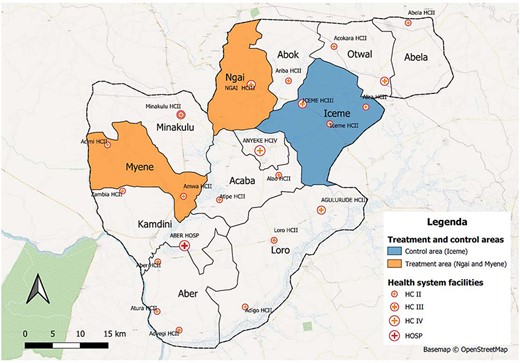
Map of Oyam district with intervention areas
The survey questionnaire contained information on a wide range of individual and household characteristics; these included demographic and socioeconomic attributes, health conditions and expenditures, perceptions about health and risk-sharing and coping strategies in response to negative shocks. Specifically, the health module gathered information on health status, utilization of health services and related costs for each household member. The recall period for out-patient healthcare was 1 month preceding the survey and 12 months in the case of in-patient healthcare. The module recorded health expenditure distinguishing between transport costs and consultation or drug costs for each episode of illness. During the second round, it was enquired whether the household received sensitization and, eventually, whether they decided to enrol. The research team conducting the survey data collection was headed by one of the authors and composed of seven enumerators and two supervisors. Participants were interviewed using smart devices, which permitted to gather georeferenced information. All interviews were conducted in the local language and took place with respect to anonymity.
Structured focus group discussion
Four SFGDs were carried out during the second round of data collection in the intervention area. These were functional to integrate and complement data from the household survey. Participants of SFGDs were purposively selected in order to create a quite representative and heterogenous sample of enrolled members. Each discussion involved 12 individuals who decided to join the intervention and were willing to share their opinion on it. Participants differed in terms of age, gender and socioeconomic position: during two SFGDs, female and men participants were equally distributed (6 and 6 in each discussion), while other two discussions involved exclusively women (12 in each discussion).1 Age of participants ranged from 19 to 67 years (with an average of 39 years), and the great majority of them (∼85%) were subsistence farmers without an additional source of income. Participants included, among others, local political and religious leaders, representatives from women’s group and members of village health teams. In total, SFGDs were attended by 48 individuals, all coming from different villages where the intervention was in place. Each discussion was conducted by two facilitators and one note-taker in the intervention area.
In order to perform a participatory exercise to evaluate the impact of the intervention, the research team applied a tool that is often associated with the capability approach: the Opportunity Gap Score matrix.2 This matrix, which is explained in detail elsewhere (Biggeri and Ferrannini, 2014), was built on the ground and used to identify the level of capability (intended as ability and opportunity) to access healthcare when needed, without anxiety and impoverishment related to health expenditures. Participants were requested to discuss and assign a score to the level of capability enjoyed by the population ranging from 0 (enjoying no opportunity at all) to 10 (enjoying the maximum level of opportunity). During the ranking exercise, four household categories were considered, including (1) rich household part of community groups and enrolled, (2) poor household part of community groups and enrolled, (3) rich household not part of community groups (and not enrolled) and (4) poor household not part of community groups (and not enrolled). Specifically, participants were requested to be quasi-impartial spectators and to assign to each household category a score according to different scenarios. These scenarios referred to the situation 1 year before (previous to the intervention in early 2019), the current situation (after the intervention in early 2020) and a counterfactual situation without the programme (how it would have been without the implementation of zero-interest loans for health).
During the SFGDs, the scoring system was explained to participants and debated. The final specification of the score in each matrix cell (i.e. the level of opportunity assigned to specific households in a specific scenario) resulted from a process of collective discussion and enquiry while considering different points of views. Overall, the exercise permitted to identify the perceived intertemporal change in the level of opportunity attributed to the intervention and, thus, to compare the results from quantitative estimates with the opinions of enrolled members.
Variables and empirical strategy
The econometric analysis sought to measure the effects of zero-interest loans for healthcare on household welfare by focusing on health expenditures and coping strategies. Accordingly, we considered as outcome variables (1) the incidence of catastrophic health expenditures, (2) the share of health costs over total monthly consumptions and (3) the incidence of financial hardship due to health costs. First, following similar studies (Karan et al., 2017), health expenses were considered as catastrophic in case they amounted to at least 25% of households’ non-food monthly expenditures.3 Second, the share of health costs constitutes an alternative measure for health expenses, and it refers to the total household consumptions. Third, financial hardship is related to the adoption of costly coping strategies in response to illness costs. These strategies involve selling household assets, borrowing with interest rates and increasing causal labour by family members. Estimates of financial hardship considered less observations, given that observing this specific outcome was conditional upon the utilization of health services.
Different household and household head characteristics were then included in the regressions as controls. Attributes concern the socioeconomic profile of the household (wealth tertiles and additional source of income different from subsistence farming), demographics (household size), number of negative shocks affecting the household during the previous year, gender, age and literacy status of the household head.
Since receiving the programme offer was conditional to being part of one community group, only a sub-sample composed of 226 eligible households, meaning those who were part of at least one community group in 2019, was included in the evaluation analysis not to introduce a bias in the estimation. In other words, households who were not part of groups at the baseline, accounting for almost 20% of the representative population sample, were not included in the main analysis. As verified with a comparison t-test (Supplementary Appendix 3), this population sub-group differs systematically from the rest of the population with respect to several socioeconomic and demographic characteristics and, consequently, cannot be easily compared with other households.4 However, in order to test the robustness of our results, we also performed a robustness check of the estimates where we considered the population not part of groups as part of the control arm.
The baseline observable characteristics (Table 1) point out a general balance across the treatment and control groups except for a minor gap regarding the existence of an additional source of income and the number of negative shocks. To adjust for this minimal bias and improve the group balance delivered by the cluster randomization approach, inverse probability weights were computed and included in the regression models.
Observables among treatment (offered programme) and control (not offered programme) groups
| Mean | ||||
|---|---|---|---|---|
| Control | Treatment | Difference | Standard errors | |
| Model variables | ||||
| (1) Catastrophic health expenditure | 0.324 | 0.382 | −0.058 | 0.068 |
| (2) Share health expenditure | 0.191 | 0.192 | −0.001 | 0.031 |
| (3) Financial hardship | 0.492 | 0.413 | 0.079 | 0.078 |
| First wealth tertile (poor) | 0.527 | 0.474 | 0.053 | 0.071 |
| Second wealth tertile (average) | 0.149 | 0.230 | −0.081 | 0.057 |
| Third wealth tertile (rich) | 0.324 | 0.296 | 0.028 | 0.066 |
| Other income sources | 0.216 | 0.118 | 0.098* | 0.050 |
| Household size | 5.541 | 5.901 | −0.360 | 0.299 |
| Shocks | 3.703 | 3.230 | 0.473* | 0.245 |
| Female HH head | 0.189 | 0.118 | 0.071 | 0.049 |
| Age HH head | 44.459 | 42.362 | 2.097 | 2.016 |
| Illiterate HH head | 0.203 | 0.151 | 0.052 | 0.053 |
| Additional variables | ||||
| Household members using outpatient services during the previous month | 1.912 | 1.822 | 0.097 | 0.222 |
| Household members using inpatient services during the previous year | 0.716 | 0.586 | 0.130 | 0.124 |
| Observations | 74 | 152 | ||
P < 0.01.
P < 0.05.
P < 0.1.
HH= household
Therefore, the intention-to-treat (ITT) effect and the average treatment effect on the treated (ATET) were estimated. The ITT effect was measured as the impact of the programme on households who were offered the intervention during sensitization, regardless of whether they decided to enrol. Conversely, the ATET considered only those who effectively participated in the scheme as the treatment group, thus including non-compliers in the control group (Table 2). In this case, the ATET and the local average treatment effect (LATE) were equal because no household in the control group accessed the programme and compliance in the treatment group were imperfect. In addition, since the uptake of the programme (enrolment ratio) was high among the sensitized population, we expected the ITT to be a lower bound of the ATET with a good level of approximation (Acharya et al., 2013).
Treatment and control groups
| Assigned treated (sensitization and offer) | ||||
|---|---|---|---|---|
| No (Z = 0) | Yes (Z = 1) | Total | ||
| Effective treated (uptake) | No (T = 0) | 74 | 28 | 102 |
| Yes (T = 1) | 0 | 124 | 124 | |
| Total | 74 | 152 | 226 | |
| Assigned treated (sensitization and offer) | ||||
|---|---|---|---|---|
| No (Z = 0) | Yes (Z = 1) | Total | ||
| Effective treated (uptake) | No (T = 0) | 74 | 28 | 102 |
| Yes (T = 1) | 0 | 124 | 124 | |
| Total | 74 | 152 | 226 | |
The ITT and the ATET were estimated using ordinary least squares and two-stage least squares, respectively. Logistic regression and bivariate probit methods were used to confirm the results for the two binary outcomes (catastrophic health expenditures and financial hardship). All models were estimated by applying robust clustered standard errors to adjust for spatially correlated shocks (Angrist and Pischke, 2008).
A few limitations regarding the econometric analysis need to be acknowledged here. First, although focusing on the sub-sample of eligible households who were already part of community groups during the baseline data collection was fundamental to validate the analysis, this did not allow us to generalize our findings to the whole population. Households who are not members of informal groups (∼20% of the population) are excluded from the interpretation of the main results, thus reducing external validity. To test the robustness of results with respect to the overall population, additional regressions have been computed, including all the 285 observations, thus also considering non-eligible households who were not part of community groups at the baseline. A second limitation regards the outcome of financial hardship that is conditional on utilization of services; this prevented capturing episodes when care was not sought although needed. Finally, the sample size did not allow to perform an appropriate heterogeneity analysis to test whether the impact of the programme is different for specific household categories and whether it induced any spillover effects on households who were not directly involved in the pilot project. While the qualitative investigation was not capable of fixing these limits, it provided some useful insights into the effectiveness of the programme with explicit reference to different household categories.
Results and discussion
Econometric estimates
The effects of the randomized offer to enrol (ITT) are presented in Table 3. The results on catastrophic health expenditures and financial hardship are statistically significant at 1% level, while those on the share of health expenditures are significant at the 2% level. All estimates are robust to the inclusion of controls. The ITT coefficients show that receiving sensitization and having the chance to enrol in the scheme decreases the incidence of catastrophic spending by almost 18 percentage points with respect to not receiving sensitization. In terms of the share of health expenditure, this is reduced by 4 percentage points due to the assignment to treatment. The incidence of financial hardship is also reduced by almost 22 percentage points in case the household received sensitization.
Effects of the randomized offer (intention to treat)
| Catastrophic health expenditures | Share health expenditures | Financial hardship | |||||||
|---|---|---|---|---|---|---|---|---|---|
ITT | −0.170*** | −0.175*** | −0.177*** | −0.0394* | −0.0385* | −0.0385** | −0.218*** | −0.217*** | −0.215*** |
(0.0474) | (0.0446) | (0.0454) | (0.0203) | (0.0197) | (0.0176) | (0.0741) | (0.0668) | (0.0716) | |
Household | |||||||||
Catastrophic health expenditure 2019 | 0.118*** (0.0380) | 0.114*** (0.0393) | |||||||
Share health expenditure 2019 | 0.0182 (0.0334) | 0.00470 (0.0358) | |||||||
Financial hardship 2019 | 0.0694 (0.0813) | 0.0673 (0.0705) | |||||||
First wealth tertile (poor) | Ref | Ref | Ref | ||||||
Second wealth tertile (average) | 0.0807 | 0.0949 | 0.00975 | 0.0145 | 0.219** | 0.224** | |||
(0.0649) | (0.0689) | (0.0179) | (0.0174) | (0.0969) | (0.0957) | ||||
Third wealth tertile (rich) | −0.00006 | −0.0181 | 0.00225 | 0.00736 | 0.160** | 0.127 | |||
(0.0566) | (0.0638) | (0.0195) | (0.0141) | (0.0655) | (0.0803) | ||||
Other income sources | −0.193*** | −0.190*** | −0.0240** | −0.0179 | −0.0263 | 0.0160 | |||
(0.0269) | (0.0291) | (0.0111) | (0.0129) | (0.0783) | (0.0767) | ||||
Household size | −0.00633 | −0.0121 | −0.0143*** | −0.0127*** | 0.0114 | 0.00408 | |||
(0.0127) | (0.0143) | (0.00516) | (0.00468) | (0.0142) | (0.0137) | ||||
Shocks | 0.0104 | 0.00802 | −0.00221 | −0.00112 | 0.00939 | 0.00812 | |||
(0.0127) | (0.0137) | (0.00507) | (0.00447) | (0.0171) | (0.0175) | ||||
Household head | |||||||||
Female HH head | 0.00772 | 0.0645** | −0.00927 | ||||||
(0.0485) | (0.0301) | (0.0898) | |||||||
Age HH head | 0.00366** | 0.00002 | 0.00411 | ||||||
(0.00182) | (0.000392) | (0.00379) | |||||||
Illiterate HH head | −0.0544 | 0.0520** | 0.0652 | ||||||
(0.0636) | (0.0254) | (0.0762) | |||||||
Constant | 0.365*** | 0.340*** | 0.237** | 0.161*** | 0.248*** | 0.216*** | 0.726*** | 0.498*** | 0.366* |
(0.0370) | (0.0818) | (0.108) | (0.0194) | (0.0486) | (0.0450) | (0.0333) | (0.135) | (0.189) | |
Observations | 226 | 226 | 158 | ||||||
R2 | 0.036 | 0.087 | 0.099 | 0.026 | 0.096 | 0.172 | 0.050 | 0.097 | 0.113 |
Note: Clustered robust standard errors in parentheses.
P < 0.01.
P < 0.05.
P < 0.1.
Observing the effects of other household characteristics on the three outcomes, we found that recording catastrophic health spending during the first round of data collection is positively associated with the probability of incurring catastrophic expenses during the second round. Indeed, the nature of vulnerability against unpredictable health costs is likely to be path-dependent over time. An additional source of income, on the contrary, presents a negative correlation with the incidence of catastrophic spending. Other attributes, which are significantly associated with an increase in the share of health expenses over total expenditures, include a lower household size and a female or illiterate household head leading to a higher share of health expenditures. We can interpret these findings considering that families headed by a woman or an illiterate individual are more likely to show greater vulnerability to income shocks, thus a higher proportion of health expenditures compared with other consumption items. A bigger household size, on the other hand, might imply a higher share of consumption devoted to different things, such as food or education. Finally, belonging to the second or third wealth tertiles with respect to the first poorest one implies a lower probability of financial hardship. This confirms the relevance of the socioeconomic status to determine the level of household vulnerability against health costs.
Estimates of the effects of the intervention uptake (ATET) are provided in Table 4. Significance levels do not change and, as expected, ATET coefficients are greater than those of the ITT effects, meaning that the impact of the programme is higher when considering members who are effectively enrolled. Participating in the programme leads to a decrease in the incidence of catastrophic spending by 22 percentage points. The share of health expenditures and the incidence of financial hardship are reduced by 5 and 27 percentage points due to the programme uptake, respectively. As in the case of the ITT effect, other factors significantly associated with the three outcomes include the previous experience of catastrophic spending, socioeconomic indicators, household size, gender and literacy status of the household head.
Effects of the uptake of the intervention (average treatment effect on treated)
| Catastrophic health expenditures | Share health expenditures | Financial hardship | |||||||
|---|---|---|---|---|---|---|---|---|---|
| ATET | −0.210*** | −0.217*** | −0.218*** | −0.0486** | −0.0476** | −0.0475** | −0.270*** | −0.270*** | −0.268*** |
| (0.0590) | (0.0538) | (0.0546) | (0.0245) | (0.0232) | (0.0205) | (0.103) | (0.0917) | (0.0968) | |
| Household | |||||||||
| Catastrophic health expenditure 2019 | 0.118*** | 0.114*** | |||||||
| (0.0373) | (0.0384) | ||||||||
| Share health expenditure 2019 | 0.0183 | 0.00438 | |||||||
| (0.0337) | (0.0354) | ||||||||
| Financial hardship 2019 | 0.0631 | 0.0591 | |||||||
| (0.0767) | (0.0681) | ||||||||
| First wealth tertile (poor) | Ref | Ref | Ref | ||||||
| Second wealth tertile (average) | 0.0903 | 0.105 | 0.0119 | 0.0168 | 0.237** | 0.243** | |||
| (0.0639) | (0.0674) | (0.0171) | (0.0168) | (0.103) | (0.104) | ||||
| Third wealth tertile (rich) | 0.0213 | 0.00821 | 0.00694 | 0.0131 | 0.182*** | 0.154** | |||
| (0.0515) | (0.0576) | (0.0189) | (0.0132) | (0.0568) | (0.0656) | ||||
| Other income sources | −0.186*** | −0.187*** | −0.0225** | −0.0172 | −0.00906 | 0.0256 | |||
| (0.0259) | (0.0275) | (0.0108) | (0.0124) | (0.0677) | (0.0688) | ||||
| Household size | −0.00679 | −0.0116 | −0.0144*** | −0.0126*** | 0.00971 | 0.00331 | |||
| (0.0113) | (0.0125) | (0.00507) | (0.00461) | (0.0153) | (0.0142) | ||||
| Shocks | 0.00436 | 0.00239 | −0.00354 | −0.00234 | 0.00234 | 0.00130 | |||
| (0.0118) | (0.0127) | (0.00500) | (0.00442) | (0.0200) | (0.0201) | ||||
| Household head | |||||||||
| Female HH head | 0.0351 | 0.0705** | 0.0196 | ||||||
| (0.0484) | (0.0289) | (0.115) | |||||||
| Age HH head | 0.00327* | −0.00006 | 0.00378 | ||||||
| (0.00169) | (0.000406) | (0.00352) | |||||||
| Illiterate HH head | −0.0621 | 0.0503** | 0.0448 | ||||||
| (0.0644) | (0.0243) | (0.0915) | |||||||
| Constant | 0.365*** | 0.353*** | 0.257*** | 0.161*** | 0.251*** | 0.220*** | 0.726*** | 0.524*** | 0.400** |
| (0.0366) | (0.0770) | (0.0993) | (0.0192) | (0.0481) | (0.0452) | (0.0329) | (0.139) | (0.189) | |
| Observations | 226 | 226 | 158 | ||||||
| R2 | 0.036 | 0.087 | 0.099 | 0.013 | 0.083 | 0.163 | 0.006 | 0.057 | 0.072 |
Note: Clustered robust standard errors in parentheses.
P < 0.01.
P < 0.05.
P < 0.1.
HH= household
Robustness checks
The results from the logistic and bivariate probit regressions (Table 5) confirm the effects of the programme on the incidence of catastrophic health expenditures and financial hardship. The impact on the two considered outcomes is highly significant, and marginal effects indicate nearly the same measures of the ITT and ATET coefficients.
Effects on catastrophic health expenditures and financial hardship using logit and bivariate probit regressions
| Intention to treat | Average treatment effect on treated | ||||||||
|---|---|---|---|---|---|---|---|---|---|
| Catastrophic health expenditures | Financial hardship | Catastrophic health expenditures | Financial hardship | ||||||
| Logit | Marg effects | Logit | Marg effects | Probit | Marg effects | Probit | Marg effects | ||
| ITT | −0.967*** | −0.175*** | −0.999*** | −0.209*** | ATET | −0.684*** | −0.210*** | −0.741*** | −0.253*** |
| (0.237) | (0.0428) | (0.334) | (0.0637) | (0.160) | (0.0478) | (0.274) | (0.0848) | ||
| Controls | Yes | Yes | Yes | Yes | Controls | Yes | Yes | Yes | Yes |
| Observations | 226 | 158 | Observations | 226 | 158 | ||||
Note: Clustered robust standard errors in parentheses.
P < 0.01.
P < 0.05.
P < 0.1.
Moreover, the main estimates on the three outcomes have been repeated considering the overall sampled population: by including households not part of community groups at the baseline (thus not eligible for the treatment) in the control group, we obtain an indication about the effects of the intervention on the general population. Some imbalances exist in this case across treatment and control groups since the intervention has not been offered randomly on the entire population; after adjusting for this potential bias through inverse probability weights,5 regressions for ITT and ATET point out results similar to those obtained on the eligible population (Tables 6 and 7). As shown for the ITT, receiving the chance to enrol into the scheme leads to a decrease in the incidence of catastrophic health expenditures by 16 percentage points, while the share of health spending and the incidence of financial hardship are reduced by almost 4 and 21 percentage points with respect to not receiving the chance, respectively. Estimates for the ATET point out very similar results to those obtained on the eligible population, recording a decline in the incidence of catastrophic spending by 21 percentage points, in the share of health expenses by 5 percentage points and in the incidence of financial hardship by 25 percentage points.
Intention-to-treat estimates including non-eligible households into the control group
| Catastrophic health expenditures | Share health expenditures | Financial hardship | |
|---|---|---|---|
| ITT | −0.163*** | −0.0377* | −0.205** |
| (0.0492) | (0.0193) | (0.0827) | |
| Household | |||
| Catastrophic health expenditure 2019 | 0.130*** (0.0416) | ||
| Share health expenditure 2019 | 0.0167 (0.0264) | ||
| Financial hardship 2019 | 0.0464 (0.0769) | ||
| First wealth tertile (poor) | Ref | Ref | Ref |
| Second wealth tertile (average) | 0.0652 (0.0697) | −0.00827 (0.0165) | 0.176*** (0.0521) |
| Third wealth tertile (rich) | 0.0322 (0.0673) | 0.000814 (0.0230) | 0.0483 (0.0586) |
| Other income sources | −0.176*** (0.0248) | −0.0108 (0.00966) | 0.0358 (0.0617) |
| Household size | −0.0145 | −0.0153** | 0.00242 |
| (0.0123) | (0.00600) | (0.0134) | |
| Shocks | 0.00707 | −0.000637 | 0.0202 |
| (0.0161) | (0.00414) | (0.0182) | |
| Membership comm groups | 0.0645 (0.106) | 0.0452*** (0.0160) | −0.00171 (0.0930) |
| Household head | |||
| Female HH head | −0.00422 (0.0454) | 0.0384** (0.0188) | −0.0671 (0.110) |
| Age HH head | 0.00375*** | 0.000643 | 0.00540*** |
| (0.00130) | (0.000426) | (0.00198) | |
| Illiterate HH head | −0.0223 (0.0514) | 0.0416 (0.0300) | 0.108 (0.0670) |
| Constant | 0.140 | 0.167*** | 0.294 |
| (0.145) | (0.0405) | (0.185) | |
| Observations | 285 | 285 | 188 |
| R2 | 0.093 | 0.143 | 0.118 |
Note: Clustered robust standard errors in parentheses.
P < 0.01.
P < 0.05.
P < 0.1.
HH= household
Average treatment effect on treated including non-eligible households into the control group
| Catastrophic health expenditures | Share health expenditures | Financial hardship | |
|---|---|---|---|
| ATET | −0.201*** | −0.0466** | −0.254** |
| (0.0602) | (0.0226) | (0.112) | |
| Household | |||
| Catastrophic health expenditure 2019 | 0.131*** (0.0408) | ||
| Share health expenditure 2019 | 0.0158 (0.0262) | ||
| Financial hardship 2019 | 0.0382 (0.0698) | ||
| First wealth tertile (poor) | Ref | Ref | Ref |
| Second wealth tertile (average) | 0.0784 (0.0720) | −0.00520 (0.0165) | 0.194*** (0.0587) |
| Third wealth tertile (rich) | 0.0422 (0.0625) | 0.00308 (0.0229) | 0.0675 (0.0574) |
| Other income sources | −0.173*** (0.0234) | −0.0101 (0.00927) | 0.0420 (0.0564) |
| Household size | −0.0141 | −0.0152** | 0.00148 |
| (0.0108) | (0.00597) | (0.0146) | |
| Shocks | 0.00277 | −0.00163 | 0.0152 |
| (0.0151) | (0.00413) | (0.0208) | |
| Membership comm groups | 0.0637 (0.100) | 0.0450*** (0.0153) | −0.00352 (0.0879) |
| Household head | |||
| Female HH head | 0.0138 (0.0503) | 0.0426** (0.0185) | −0.0459 (0.132) |
| Age HH head | 0.00354*** | 0.000597 | 0.00519*** |
| (0.00124) | (0.000432) | (0.00184) | |
| Illiterate HH head | −0.0316 (0.0562) | 0.0395 (0.0291) | 0.0904 (0.0809) |
| Constant | 0.153 | 0.170*** | 0.321* |
| (0.141) | (0.0407) | (0.180) | |
| Observations | 285 | 285 | 188 |
| R2 | 0.083 | 0.134 | 0.081 |
Note: Clustered robust standard errors in parentheses.
P < 0.01.
P < 0.05.
P < 0.1.
Focus group findings
The performance of SFGDs allowed us to verify that the community opinions about the impact of the intervention were in line with the estimated effects. Indeed, in all the four discussions, an improvement in the opportunity to access healthcare was identified and attributed to the zero-interest loans for healthcare. The perceived change in the opportunity level appears heterogeneous with respect to different household categories. Considering households that are part of community groups targeted by the intervention, the average opportunity score shows an increase of 100% (from 3 in early 2019 to 6 in early 2020) for poor households and an increase of 33% (from 6 to 8) for rich households. Considering the population not enrolled into the scheme, the intertemporal increase in the average score is less pronounced in absolute terms, rising from 1 to 2 for the poor and from 5 to 6 for the rich. Participants agreed on the fact that the contribution provided by the programme to raise the opportunity score had been substantial for group members, especially for those not having other means to meet unpredictable health expenses, namely, the poor.
As we take into account the opportunity scores assigned to the counterfactual scenario, participants argued that a minimal increase would have had occurred regardless of the intervention since households always seek to improve their living standards: a potential increase of 33% (from 3 to 4) and 17% (from 6 to 7), respectively, for poor and rich household part of community groups and a potential increase of 50% (from 1 to 1.5) and 20% (from 5 to 6), respectively, for poor and rich households not part of community groups were observed. Overall, it is possible to calculate the perceived net impact of the intervention by considering the difference between the intertemporal change and the counterfactual scenario as observed by participants. For poor and rich households enrolled into the scheme, the net effect of the programme on the opportunity level is a perceived increase of 50% and 17%, respectively. Moreover, for poor households not enrolled into the scheme, there is a perceived net increase of 33% in the opportunity level due to the programme (spillover effect). No real change is identified for rich households not enrolled into the scheme.
Findings from this exercise were the same during all four SFGDs and suggested two main points about the heterogeneity of the effects. A first distinction regards membership to informal groups targeted by the programme. The community clearly perceives the benefits obtained by the target population through the intervention. Participants argued that some positive spillover effects could occur at the village level when households not part of the scheme learn from their neighbours about the practice of saving for health expenses.6
Maybe poor families not part of group received some messages from friends who are part of the scheme, so there is a small effect also for them. If they get little information about being prepared for health issues, they may start to save some money[for this].
However, without access to the common pool of resources, the impact remains minimal. A pre-existing difference between being or not being part of a targeted community group is also evident: households not members of community groups were identified as more vulnerable against health shocks. Such a difference was often explained during the SFGDs when referring to solidarity and mutual help practices, which have some potential to alleviate the burden of unpredictable expenses7:
For a poor family not part of any group it is very difficult to use services, because there is no external support, and also they don’t have assets to sell out in case of need. […] For a rich family not part of any group the opportunity is worse than for a rich family part of a group, because they depend only on their money and assets, while they don’t have support from others.
The second distinction concerns the opportunity level enjoyed by poor and rich households enrolled into the scheme: all members record an improvement due to the programme, but the change for the poor is perceived as relatively greater. Participants argued that, on the one hand, the rich already have some means to meet health expenditures, and membership to the intervention represents an additional safety strategy for them. On the other hand, for the poor who do not own significant assets or savings, the new possibility to rely on the scheme funds considerably improves their situation in case of need8:
The contribution of the program for rich families is lower [than for poor families] because they have already their money, they can also sell out things, they don’t depend exclusively on the group. […] Poor people can borrow from the scheme and this is the only solution for them.
Conclusions
This paper examines the impact of the initial phase of a CHF pilot scheme on health expenditures and coping strategies in a rural context of Uganda. The analysis is based on a panel household survey and exploits the randomization of the offer to enrol in the pilot scheme as a valid instrumental variable for the treatment status. Our approach allowed us to avoid selection bias and to obtain reliable estimates of the ITT effect on sensitized households and the ATET on effectively enrolled members. As shown by the results, the programme led to a significant decrease in the incidence of health expenditures, as well as of the share of health expenses, and of the occurrence of financial hardship. Estimates are robust and indicate that the intervention is effective in improving households’ financial protection and in reducing the adoption of costly coping strategies in response to unpredictable health costs. The effect on financial hardship also suggests longer-term benefits in mitigating vulnerability to other forms of shocks. The results are consistent with existing studies on CHF arrangements in different contexts (Aggarwal, 2010; Chankova et al., 2008; Dror et al., 2016; Galárraga et al., 2010; Jütting, 2004; Mebratie et al., 2019; Savitha and Kiran, 2015) and add to the body of the evaluation literature that mainly relies on longitudinal data.
Core findings obtained through the econometric analysis are confirmed by the community perceptions expressed during the SFGDs. Qualitative evidence provides valuable clues to acknowledge the heterogeneity of the impact on different household categories. Consistent with other studies (Jütting, 2004; Umeh and Feeley, 2017), structured focus group findings suggest that more disadvantaged people in terms of access to healthcare are excluded from participating in the scheme (as confirmed by the quantitative comparison presented in Supplementary Appendix 3), thus raising equity concerns on the impact of the intervention. Among enrolled members, the poorest are likely to receive greater benefits from the scheme. This point is not in line with existing quantitative evidence on a higher impact of health insurance on the richer (Wagstaff et al., 2009; Woldemichael et al., 2019). However, our findings concern zero-interest loans for health, and this may suggest that the initial phase of the CHF programme implies specific heterogeneity effects. Although external validity of our results holds only in the context of Oyam district, it is reasonable to suppose that patterns to access health services and to cope with health expenses are not much different among rural households participating in informal community groups in Uganda and in other LMICs. Consequently, the presented evidence suggests that encouraging health savings arrangements at the village level has the potential to significantly improve financial protection and coping strategies in response to illness in similar settings.
Overall, our analysis provides support for the positive role of community-based mechanisms to progress towards UHC and brings forward important policy considerations. Models of CHF and zero-interest loans for healthcare represent an initial and preliminary step in the implementation of a comprehensive insurance platform. Catalysing demand for financial protection through informal community groups is extremely useful to set up the scheme, while creating awareness on the harmful effects of financial hardship and benefits of risk-sharing. However, careful attention is required to meet equity objectives when designing the upgrade and scaling up of the CHF intervention. In fact, it is crucial to extend the target of the scheme to the whole population in the informal sector, and this is possible only by complementing community-based arrangements with tailored subsidies provided by the government for the poorest. In conclusion, this type of intervention alone does not constitute a valid solution for achieving universal coverage but has the potential to trigger an effective improvement in this direction. In order to be sustainable over time and meet the ultimate goal of UHC, the transition needs to be supported by a clear stewardship from the public sector to ensure equity and coordination in the insurance management.
Supplementary data
Supplementary data are available at Health Policy and Planning online.
Data availability statement
The data underlying this research cannot be shared publicly for the privacy of individuals that participated in the study. The data will be shared on reasonable request to the corresponding author.
Funding
The authors received no financial support for the research from any external funding body. Technical and logistical support for the data collection in Uganda was provided by Doctors with Africa CUAMM.
Acknowledgements
We are grateful for the logistical support provided by CUAMM in Uganda. We benefited from the research support of Fabrizia Mealli and Bruno Arpino and from the comments and suggestions of Gavino Maciocco. We would like to thank the Oyam district authorities for their support during the fieldwork and the members of the research team. We would also like to thank the people of Oyam who participated in the survey with patience and courtesy.
Ethical approval
Ethical approval for the study was obtained by the Uganda National Council for Science and Technology (ref: SS 5122), and informed written consents were collected from all research participants.
Conflict of interest statement
The authors declare that they have no conflict of interest.
Endnotes
The composition of these two SFGDs was intended to capture women’s view without the risk of power imbalances among participants.
The method of SFGD using the Opportunity Gap Score matrix combines the classical setting of a focus group with a matrix scoring system (Catley et al., 2008) involving a sequence of steps and questions that are largely fixed and therefore replicable in a clear and defined way to achieve comparability of findings. Supplementary Appendix 1 reports the structure of the matrix applied during SFGDs and the aggregated results obtained during the four SFGDs.
Supplementary Appendix 2 also presents the results for the outcome of catastrophic health expenditures when the threshold of 10% of total household expenses is considered. Estimates obtained with the two alternative cut-off points are compared, showing that the 25% cut-off permits to capture a more significant change.
Supplementary Appendix 3 presents statistics on differences with respect to observable characteristics between households who are members of community groups and those who are not part of community groups. Statistics indicate that excluded households are more likely to be poor, to have a lower household size and to be headed by women and illiterate people. Moreover, as shown elsewhere (Biggeri et al., 2018a), this group presents a lower level of willingness to join CHF arrangements.
Further to inverse probability weights, these regressions include an additional control variable for the membership to community groups.
A participant during SFGD in Ngai sub-county, 21 January 2020.
A participant during SFGD in Myene sub-county, 23 January 2020.
A participant during SFGD in Myene sub-county, 24 January 2020.
