


Abstract
This study presents for the first time the SWB-J index, a subjective well-being indicator for Japan based on Twitter data. The index is composed by eight dimensions of subjective well-being and is estimated relying on Twitter data by using human supervised sentiment analysis. The index is then compared with the analogous SWB-I index for Italy in order to verify possible analogies and cultural differences. Further, through structural equation models, we investigate the relationship between economic and health conditions of the country and the well-being latent variable and illustrate how this latent dimension affects the SWB-J and SWB-I indicators. It turns out that, as expected, economic and health welfare is only one aspect of the multidimensional well-being that is captured by the Twitter-based indicator.
1. Introduction
The improvement of social well-being explicitly entered the policymaker agenda a few decades ago, when it became clear that objective measures of observable quantities – above all, GDP – were unsatisfactory proxies of the welfare conditions of a community (Stiglitz et al. 2009). As a consequence, instruments for measuring and monitoring social well-being began to appear in the toolbox of policymakers, progressively moving the focus from objective to subjective evaluation: multidimensional indicators encompassing both objective and subjective dimensions of well-being (Barrington-Leigh and Escande 2018; Fleurbaey 2009), face-to-face or telephone surveys investigating samples of citizens about their own perception of quality life (Kahneman et al. 2004; Schwarz and Strack 1999), and, after the development of the internet, the application of several techniques to the analysis of individual and collective mood through large-scale data provided by social networking sites (SNS), with the aim of drawing an evaluation of well-being status from conversations (Luhmann 2017; Scollon 2018) or word search (van der Wielen and Barrios 2021) on the web.
In this context, Twitter is one of the most popular SNS, with about 330 million monthly active users worldwide in 2019 (according to Statista.com, see https://www.statista.com/statistics/282087/number-of-monthly-active-twitter-users/). Due to the brevity of the messages allowed and the huge number of tweets potentially available and continually updated, the platform has been considered one of the most suitable information sources to estimate emotional well-being, i.e. the ‘mood’ or short-run component of the life quality evaluation.
Recent literature provides some examples of well-being evaluations that rely on Twitter data and, based on sentiment analysis methods, aim at monitoring the day-by-day evolution of self-declared emotional status of a community.
In particular, Dodds et al. (2011) built a happiness indicator, called the hedonometer, based on a so-called ‘closed vocabulary’ approach: they measured the frequency of use of a set of ten thousand words for which they obtained happiness evaluations on a nine-point scale, using Amazon Mechanical Turk (see online documentation at https://www.mturk.com/). Their dataset was huge, comprised of around 4.6 billion expressions posted by over 63 million Twitter users from September 2008 to September 2011. The project is still ongoing, and the hedonometer is now evaluated daily by the University of Vermont Complex Systems Center, which can thus provide a time series from 2008 (on-line plots are available at https://hedonometer.org/timeseries/en_all/).
A subjective well-being indicator – named the Gross National Happiness Index – has been proposed by Rossouw and Greyling (2020); the indicator has been evaluated since 2019 in three Commonwealth member countries: South Africa, New Zealand and Australia (an on-line dashboard is available at https://gnh.today). The aim of the project is to measure, in real time, the sentiment of countries’ citizens during different economic, social and political events. Its first application was an examination of the well-being impact of social restrictions imposed during the first wave of the Covid-19 pandemic in South Africa (Greyling et al. 2020). In order to calculate the index, sentiment analysis is applied to a live Twitter-feed, and each tweet is assigned either a positive, neutral or negative sentiment. Then, an algorithm evaluates a happiness score on a 0-to-10 scale. The Gross National Happiness Index provides a happiness score per hour for each of the three countries.
Several other studies apply sentiment analysis to the data provided by Twitter in order to monitor short-run levels of happiness (Bollen et al. 2017) but also life satisfaction, defined as a medium-long run evaluation of life quality (Schwartz et al. 2013; Yang and Srinivasan 2016; Lim et al. 2018; Durahim and Coşkun 2015; Abdullah et al. 2015; Quercia et al. 2012; Greco and Polli 2020). We acknowledge that Twitter is not a representative sample of any society, but we also follow previous studies that have successfully shown that Twitter data effectively illustrate what occurs in the real world, ranging from elections (Ceron et al. 2014), to stock markets (Bollen et al. 2011), to public health (Fahey et al. 2020).
An algorithm for sentiment analysis, named Integrated Sentiment Analysis (iSA) (Ceron et al. 2016), is used in this work to obtain a composite subjective well-being indicator for Japan named SWB-J (Subjective Well- Being Japan). The advantage of iSA, compared to the wide range of sentiment analysis algorithms and methods applied to SNS big data repositories, is that iSA is a human-supervised machine learning method, where a sample set of texts (training set) is first read and manually classified by human coders, and then the rest of the corpus (unlabelled set) is automatically classified by the algorithm. This allows for extracting qualitative information from a text without relying on predefined dictionaries or special semantic rules – on the contrary, iSA can investigate cultural, psychological, and emotional aspects of language, grasping all the nuances of informal and colloquial expressions. The feature is particularly significant because the analogue of SWB-J has been estimated for Italy (SWB-I) (Iacus et al. 2019, 2020a,b) with the same methodology: a comparison between the two indicators may be attempted, contributing to the challenging task of disentangling differences in life quality evaluations from cultural and linguistic specificities in expressing and communicating feelings and moods.
The SWB-J Project was created in collaboration between the University of Milan and Insubria in Italy and two Japanese counterparts: The University of Tokyo and Waseda University.
The paper is structured as follows: Section 2 introduces the big data approach in the study of well-being. Section 3 briefly presents some cultural aspects of how emotions are expressed in Japanese language and reviews some recent literature on computational linguistic about extracting emotions from Japanese tweets. Section 4 describes the SNS data used in this study as well as other sources of data used in the subsequent sections, while Section 5 describes the sentiment analysis methodology used to create the SWB-J indicator. Section 6 discusses the resulting new SWB-J indicator and compares its features with the Italian counterpart SWB-I. Section 7 presents a cross-country analysis aimed at explaining what can potentially impact the different patterns of SBW-J and SWB-I through an econometric analysis. Section 8 summarizes the results and limits of this approach, and the Supplementary Appendix contains additional technical material about the construction of the index.
2. Why to Estimate Subjective Well-Being via SNS
Well-being evaluation has turned from the estimation of objective quantities to the assessment of subjective mood and state of mind because observable variables – even in a multidimensional approach – have proven inadequate to accurately account for the welfare conditions of a society (Kuznets 1934; Sen 1980). Criticism of this approach has come to question its empirical relevance and opened doors to an overturning in the strategies for well-being evaluation: if both one-dimensional and multidimensional measures are unreliable due to the limits of observable variables, the only feasible option to estimate individual and collective well-being is to explicitly ask people to express an evaluation about their own condition.
To this aim, surveys and questionnaires have been increasingly and widely used to collect information about well-being levels and dynamics of individuals and communities. Different methods to conduct surveys have been developed – also conditioned by the technology applied (face-to-face interview, telephone, internet) – in order to disentangle the incidental, emotional aspect of self-reported well-being and the evaluation of life satisfaction, which requires examining current and past events from a medium or long-run perspective.
However, survey-based research projects have a significant drawback, which is the bias induced in well-being evaluation by the survey itself. This is the sort of ‘Hawthorne effect’1 that Angus Deaton (Deaton 2012; Deaton and Stone 2016) pointed out: in fact, changing the order of the questions of a survey may be sufficient to affect the evaluation the respondents give about their own mood or quality of life. More generally, when the respondents are aware of being asked for an assessment of their own life and of being observed while giving the evaluation, the answer they give may be biased by this awareness. Therefore, the dilemma the analysts face is quite clear: on one hand, they wish to ask people for a self-evaluation of their well-being, in order to overcome deficiencies due to measurements based only on observable quantities; on the other hand, they should not ask people for a self-reported evaluation, in order to avoid biases due to the awareness of respondents.
With the era of virtual communication, a new source of large-scale data is provided that seems to address the need for this kind of information: in fact, the availability of a huge and continually updated flow of conversations on SNS theoretically provides a real-time opportunity to know what people think about the quality of their own daily life – both from an emotional and an evaluative perspective – without submitting any explicit questionnaire. This is fostering a stream of studies whose aim is to extract meaningful information from the enormous amount of words or images posted on well-known platforms such as Facebook, Twitter, and Instagram (Voukelatou et al. 2021).
In order to appreciate the kinds of information that can be drawn from SNS data when used for evaluating subjective well-being, it should be clarified that the content and meaning of subjective well-being finds different definitions. The widely accepted definitions proposed by the OECD guidelines (OECD, 2013), for instance, distinguish: (a) affect, i.e. the description of a person’s feeling or emotion, typically measured with reference to a particular point in time; (b) life evaluation, which is an assessment of life ‘as a whole’ and requires a judgment by the individual, rather than a description of an emotional state. Life evaluations are not simply the average of punctual evaluations, being – on the contrary – based on how people remember their experiences, which can differ significantly from how they actually experienced things at the time; (c) eudaimonia, which focuses on functioning and the realization of personal potential, involving elements such as autonomy, competence, interest in learning, goal orientation, sense of purpose, resilience, social engagement, caring, and altruism.
Other sources use similar definitions, such as hedonic for affect or emotional well-being (Ryan and Deci 2001; Deaton and Stone 2013; Steptoe et al. 2015). Frequently – but not exhaustively – these definitions are expressed in relation to the time span used to carry out the well-being evaluation.
Twitter – like the other social networking platforms – is usually considered a good data source for the estimation of short-run emotional well-being. This is, in fact, the dimension of subjective well-being these indicators aim to capture. This notwithstanding, Twitter has also been used in some studies to evaluate components of subjective well-being conceived as more structural, commonly indicated as life evaluation or life satisfaction (see Schwartz et al. 2013; Yang and Srinivasan 2016).
One of the main advantages of large-scale datasets coming from SNS is their continuous updating. This offers the opportunity for nowcasting.2 In fact, while variables that are more traditionally assumed to be related to welfare – such as GDP or morbidity rates – are observable only with a time lag, which sometimes makes the policymaker intervention less effective, SNS data allow for real-time monitoring of public sentiment and can anticipate changes in objective variables. Moreover, when the methods for sentiment analysis are language-independent (i.e. they can be applied to texts expressed in different languages, without any particular limitation), a comparison among linguistic and socio-cultural contexts becomes possible, revealing not only differences in the use of language, but also cultural specificities – such as social conventions that impose stricter self-control in expressing emotions – as far as they are recorded in virtual conversations.
On the other hand, SNS data also have some intrinsic limitations. First of all, users of these platforms are not representative of the whole population. Therefore, any social well-being evaluation achievable from the analysis of these data cannot be immediately extended to the whole population. Procedures can be adjusted to make the results more general; but above all, and despite their limited representativeness, SNS can be considered a sort of opinion-making arena, where expressed ideas affect or anticipate collective sentiment and trends. As Salganik (2017) mentioned, there is always a risk of drifting in constructing indicators based on social media data due to the fact that, not only is the reference Twitter population not representative, but it might also change composition over time or the users may post different volumes of tweets at different times, etc. We cannot do much in computational social science at present without, e.g. crossing Twitter accounts with panel survey data, and this was not possible in this study. Nevertheless, our SWB indicators at least are not affected by changes in the volume of data since they are based on relative measures (see equation (1) below) and further based on aggregated analysis, preventing any particular account from dominating the others.
In other words, we think that the opinions of internet users are significant per se: insofar as SNS conversations are public (i.e. the accounts are freely accessible), they can be read – easily and at a low cost – by a wide set of people and exert a sort of ‘lighthouse effect’, in that they may anticipate, affect, and shape public opinion. That is why we think that the sentiment expressed via SNS is important, even beyond its statistical representativeness. This suggests that a second drawback can be imputed to evaluation of well-being via SNS data: the use of social networks itself can alter self-perceived or self-declared well-being. In fact, even if SNS users do not answer any explicit questions about their own personal status, they are aware that they are sharing their feelings with a community, and thus they may distort their well-being self-reports in order to satisfy self-representation needs. Furthermore, SNS messages and texts seem more suitable to reflect short-term mood changes than a long-term evaluation of life quality: therefore, a well-being indicator based on SNS data would be more reliable as a measure of emotional well-being than a source of life evaluation. However, despite the validity of this remark, adequate statistical analysis can help in separating the volatile and structural components of well-being described by virtual conversations on the net.
An important issue raised by the availability of this new data source is a technological one: the increase in computational power of technological devices does not guarantee, per se, the ability to separate helpful information from background noise in virtual conversations. Following Gary King, we can say that ‘Big data is not about the data’ (King, 2016): it is rather about the opportunity to extract knowledge from data, and this requires adequate methodologies and tools. Fortunately, recent advancements in statistical theory and its applications are improving the capacity of social scientists to analyze the content of these large-scale datasets and promoting the dissemination of different methods of sentiment analysis. The subjective well-being indicator we propose in this work is based on the iSA algorithm, which is one of these new methods.
3. Expressing Emotions in Japanese Culture and SNS
As mentioned by Miyake (2007), in traditional Japanese communication, people tend to maintain distance and make sure that neither party loses face (see also Matsumoto 1999). In textual analysis, most studies focus on the identification of big corpora of web blogs or SNS posts (Ptaszynski et al. 2014) in the context of sentiment and affect analysis.
It should be noted that emoticons, or emoji, are peculiar in Japanese written digital communication. For example, before graphical emoticons appeared, in the western cultures horizontal emotions like ‘:)’ were used, while in Japan (and other Asian countries) emoticons were and are traditionally vertical, for instance ‘(`o´)’. Emojis were already installed as a standard package in the messaging platforms of mobile devices in Japan in the late 1990s (e.g. Jphone and iMode). The development of emoji is distinctive in Japan and arguably originates from ‘kanji’ culture, in which characters represent an idea or concept as a graphic symbol (which also applies to other Asian countries that employ Chinese characters). Despite the abundance of emoticons, a large cross-country study seems to prove that regardless of the culture, vertical and horizontal emoticons convey similar concepts (Park et al. 2014). Still, emoticons coupled with adverbs seem to be able to predict better than simple emoticons the affective perception of a text message (Rzepka et al. 2016).
Many other studies related to the association between emoticons and emotions can be found in the literature (e.g. Shoeb and de Melo 2020; Novak et al. 2015), but they are not specific to the Japanese language. In relation to the Japanese cultural practice of expressing emotions by non-verbal means, a graphic design known as ASCII art has been quite extensively used in bulletin boards such as 2channel (one of the most popular online bulletin boards). Personality trait estimation of Japanese Twitter accounts has been studied in Kamijo et al. (2016). Large scale studies on automatic sentiment tagging in Japanese during crisis periods can be found in Vo and Collier (2013). More linguistic analyses on specific Japanese terms related to likeness and happiness have recently appeared (for the word ‘kawaii’ see Iio 2020) as well as gender-specific language studies (Carpi and Iacus 2020).
In summary, all the current studies are either dictionary or semantic rule-based or apply some version of the classical Word2Vec approach (Mikolov et al. 2013) or standard NLP techniques (e.g. Bengio et al. 2003). In this study, as will be described in Section 5, we use a mixed qualitative and quantitative approach which tries to take into account the complexity of the well-being dimensions and the language used to express them. Indeed, the analysis does not focus on special features of a message but on the whole set of the words in a tweet after accurate training by humans who are Japanese native speakers and fully understand all the shadings of the natural language used to express emotions.
4. Data Collection
The data used in this work come from two different repositories that were collected under two different projects, in both cases using Twitter search API. The Japanese tweets were collected using only the filters on language = Japanese and country = Japan and similarly for Italy (Italian and Italy). It is worth mentioning that Twitter posts do not belong to individuals randomly chosen from a physical population (Baker et al. 2013; Murphy et al. 2014). The reference population is the population of posts of all Twitter accounts selected in the analysis. Moreover, Twitter accounts cannot be uniquely associated to individuals, and some accounts are more active than others. For these reasons, the focus of our analysis is on the total volume of the posts collected (in Japan, written in Japanese language, during the reference period) through the public Twitter ‘search’ and ‘streaming’ API (Application Programming Interface). As per the official documentation, Twitter search API only provides a 10% sample of all tweets, though the company does not disclose any information about the representativeness of the sample with respect to the whole universe of tweets posted on the social network. Nevertheless, according to our personal experience, also confirmed in large scale experiments by Hino and Fahey (2019), the coverage of topics and keywords is quite accurate and appears to be randomly selected: therefore we consider the Twitter data used in this study to be a representative sample of what is discussed on Twitter. According to Statista, there are about 8 million accounts active daily in Italy whilst about 52 million are in Japan, therefore the number of tweets posted is not comparable. Despite these limitations, the advantage of using Twitter data is that the collection of data can be done in (almost) continuous time and, moreover, instead of asking something through a web-form (thanks to the human supervised qualitative analysis explained in Section 5) it is possible to capture expressions of well-being from the texts directly.
For Italy, the original project collected about 250.4 million tweets in the period 1 Feb 2012 to 21 June 2018, with a median of 50,000 tweets per day. For Japan, for several technical reasons, we were able to collect at most 50,000 tweets a day, amounting to about 60.8 million tweets in the period 24-08-2015/31-12-2018. Table 3 reports summary statistics. In the same table, we report also the values of the Happy Planet Index (HPI) by New Economics Foundation (NEF 2016) and the Human Development Index (HDI) by the United Nations Development Programme (2019), for the same years available for the SWB-I an SWB-J indexes. Data are taken from the data provider TheGlobalEconomy (web portal for data access at https://TheGlobalEconomy.com) for the other economic variables listed in Table 1, mostly coming from The World Bank, the International Monetary Fund, the United Nations, and the World Economic Forum. We also collected from OECD the variable Life Expectancy of Males at 40, to capture the perception and quality of aging (data available at web portal: https://data.oecd.org/healthstat/). This is the only yearly variable we consider; it varies non-monotonically in time and, moreover, is also correlated positively with economy growth in Italy (ρ = 0.91) but negatively in Japan (ρ = −0.27).
Economic and Environmental Variables Used in the Econometric Analysis of Section 7 Plus Two Additional Well-being Indexes.
| Variable | Frequency | Description |
|---|---|---|
| GDP growth | Quarterly | Percent change in quarterly real GDP year on year |
| Consumption growth | Quarterly | Percent change year on year |
| Investment growth GDP | Quarterly | Percent change year on year |
| Unemployment rate | Monthly | Percentage of work force |
| Life Expectancy at 40 | Yearly | Male only |
| Happy Planet Index | Yearly | |
| Human Development Index | Yearly |
Yearly Average Values of SWB-I and SWB-J, Their Standard Deviation in Parentheses, and Number of Tweets in Millions. Data are in the Period 1 February 2012 to 21 June 2018 for Italy and 24 August 2015 to 31 December 2018 for Japan. For the Happy Planet Index (HPI) and Human Development Index (HDI), Data Was Sourced From the World Bank.
| Year | 2012 | 2013 | 2014 | 2015 | 2016 | 2017 | 2018 |
|---|---|---|---|---|---|---|---|
| SWB-I | 48.9 | 52.2 | 49.7 | 48.7 | 50.5 | 57.7 | 55.7 |
| (4.2) | (3.8) | (4.9) | (9.8) | (7.5) | (4.5) | (7.1) | |
| tweets | 44.2M | 40.8M | 34.4M | 38.3M | 55.2M | 32.6M | 14.9M |
| HPI | – | 6.02 | – | 5.95 | 5.98 | 5.96 | 6.00 |
| HDI | 0.874 | 0.873 | 0.874 | 0.875 | 0.878 | 0.881 | 0.883 |
| SWB-J | – | – | – | 54.4 | 53.6 | 53.2 | 52.5 |
| – | – | – | (13.4) | (11.1) | (13.1) | (12.7) | |
| tweets | – | – | – | 6.5M | 18.2M | 18.2M | 17.8M |
| HPI | – | – | – | 5.99 | 5.92 | 5.92 | 5.92 |
| HDI | – | – | – | 0.906 | 0.910 | 0.913 | 0.915 |
5. How to Extract Subjective Well-Being from Tweets
The SWB-J index is a multidimensional well-being indicator whose components were inspired by the dimensions suggested by the New Economic Foundation think-tank in its reports on national accounts of well-being (NEF 2009, 2012). In summary, the SWB-J mimics the same indicator SWB-I previously built for Italy (Iacus et al. 2019, 2020a, b) and consists of eight dimensions that concern three different well-being areas: personal well-being, social well-being, and well-being at work. In greater detail:
Personal well-being:
emotional well-being: the overall balance between the frequency of experiencing positive and negative emotions, with higher scores showing that positive feelings are felt more often than negative ones (emo);
satisfying life: having a positive assessment of one’s life overall (sat);
vitality: having energy, feeling well-rested and healthy while also being physically active (vit);
resilience and self-esteem: a measure of individual psychological resources, of optimism, and of the ability to deal with life stress (res);
positive functioning: feeling free to choose and having the opportunity to do it; being able to make use of personal skills while feeling absorbed and gratified in daily activities (fun);
Social well-being:
trust and belonging: trusting other people, feeling treated fairly and respectfully while experiencing sentiments of belonging (tru);
relationships: the degree and quality of interactions in close relationships with family, friends, and others who provide support (rel);
Well-being at work:
quality of job: feeling satisfied with a job, experiencing satisfaction with work-life balance, evaluating the emotional experiences of work and work conditions (wor).
Given the collectivist nature of the Japanese society, it makes sense to measure subjective well-being based on multiple dimensions encompassing social well-being and well-being at work. It is known, in fact, that personal well-being is more closely associated with social well-being and well-being at work in Japan compared to the United States (Kitayama et al. 2000; Ford et al. 2015) and – more recently – China (Wong et al. 2020). It is also known that Asian countries (in particular Pacific Rim countries (Diener et al. 1995)) tend to mark lower scores in reported subjective well-being compared to the US, but few works have attempted to measure the level of subjective well-being with social media data. Thanks to the multi-dimensional nature of the index, one can better understand and investigate the internal dynamics of subjective well-being. It should be noted that, in discussing the concept of well-being in the Japanese society, Kumano (2018) distinguishes two types of well-being: shiawase or hedonic, emotional well-being, and ikigai or eudaimonic well-being. The distinction is quite familiar also to cultures of Western countries and, as far as the different concepts of well-being impact on the daily expression of well-being, they are both captured by our indicators. It must be emphasized, however, that disentangling the hedonic or emotional component from the eudaimonic one is far beyond the scope of this work and, perhaps, beyond the potential of our indicator, which is conceived as a proper measure of hedonic well-being. Examining the relationship between emotional (as expressed on SNS) and eudaimonic well-being, if any, will be a challenge for future research.
To extract semantic meaning from tweets, in this study we use a supervised sentiment analysis method and, in particular, the iSA (Integrated Sentiment Analysis) algorithm (Ceron et al. 2016) which has been also used to capture various aspects of happiness and well-being from Twitter data (Curini et al. 2015). iSA is a human supervised machine learning method wherein a sample of texts (the training set or labelled set) is first read and manually classified by human coders, and then the rest of the corpus (the test set or unlabelled set) is automatically classified by the algorithm. The supervised part is essential in that this is the step where qualitative information can be extracted from a text without relying on dictionaries or special semantic rules but rather on cultural, psychological and emotional interpretation. To this aim, it is very important that the labelling of the texts in the training set is performed by native language speakers with a minimum of field knowledge. We will discuss in full details the coding strategy in Section 5.2. Other approaches based on user-defined dictionaries exist, but mainly focus on the concept of happiness (Bollen et al. 2011; Zhao et al. 2019). The advantage of iSA over other machine learning techniques is that it is designed to estimate directly the aggregated distribution of the opinions (e.g. positive, negative, neutral) without passing through the individual classification of posts in the unlabelled set. This approach vastly reduces the estimation error. Moreover, as iSA is a sequential method, in this context of highly noised data, the size of the training set needed to reach the same accuracy of other methods is usually smaller by a factor of 10 or 20 times. We will briefly present the main technical points of the iSA algorithm in Section 5.1, but the reader can also refer to Ceron et al. (2016) for an in-depth technical explanation of the method.
Once the training set has been completely hand-coded, the iSA algorithm is applied to daily unlabelled sets of data. Each estimated distribution will contain the entries positive, neutral, negative and Off-Topic. The Off-Topic category represents the daily noise in the data, the rest represents the signal. For each component of the index, for example emo, the index is calculated, for day d, as follows:
The rationale behind formula (1) is that the intent is to capture expressions or judgments, and this is why comments not expressing any issue, judgments, etc. – i.e. those classified as neutral – are removed from the calculation. The day d is easily extracted from the timestamp of Twitter data which is always present in the metadata of a tweet.
Finally, the SWB-J index is the simple average of the eight components emo, sat, vit, res, fun, tru, rel, and wor. Although it falls outside of the scope of this study, specific weighted averages of the components might be considered in order to obtain a well-being indicator oriented to specific life dimensions.
5.1. The iSA Classification Algorithm
Let us denote by the set possible categories (i.e. sentiments or opinions) in which we want to classify texts. Here D0 is the Off-Topic category, which is usually the most frequently observed category in unstructured data.3 We want to estimate {P(D), D in D}, i.e. the distribution of opinions in the corpus of N texts. Let Si, i = 1, …, K, be a unique vector of L possible stems (i.e. single words, unigrams, bigrams, etc.) which remain in the document-term matrix after the pre-processing4 phase which identifies one of the texts in a corpus. These vectors are sequences of zeros and ones, e.g. s1 = (1,1,1,0,0,0,0,0,0) is associated to document 1, s2 = (0,0,0,1,1,1,0,0,0) for document 2, etc. Of course, more than one document may have the same feature vector, so that, for example, S1 and S20 may both be equal to, e.g. sequence s3, etc. Each vector Si belongs to the space of 0/1 vectors of length L (the number of stems), where each element of Si is either 1 if that stem is contained in a text, or 0 in case of absence. The number of possible different rows in the document-term matrix is then K = 2^L. Most supervised machine learning methods (e.g. multinomial regression, Random Forests (RF), Support Vector Machines (SVM), and Artificial Neural Networks (ANN), just to mention a few) use the individual hand coding from the training set to construct a model P(D|S) for P(D) as a function of S to train a model that predicts the outcome of for the texts with S = sj belonging to the test set. Then, when all data have been imputed in this way, these estimated categories are aggregated to obtain a final estimate of . In matrix form:
where P(D) is a M × 1 vector, P (D| S) is a M × K matrix of conditional probabilities and P(S) is a K × 1 vector which represents the distribution of Si over the corpus of texts. Once P(D|S) is estimated from the training set with, say, is estimated with the naïve Bayes estimator as the maximizer of the conditional probability, i.e. . Following Hopkins and King (2010), the iSA idea is changing one’s point of view and focusing on what can be really and accurately estimated. Instead of equation (2), one can proceed considering this new equation:
where now P(S |D) is a K × M matrix of conditional probabilities whose elements P(S = Sk |D = Di) represent the frequency of a particular stem Sk given the set of texts which actually express the opinion D = Di. In this case, all these probabilities can be considerably well estimated if there is a sufficient number of texts in the training set which are hand coded as D = Di (Hopkins and King 2010; Ceron et al. 2016). While the original method in Hopkins and King (2010) uses a combined approach of bagging on the number of stems used in each step and a bootstrap to obtain standard errors, iSA uses all stems at the same time, reducing the computational burden as well as making possible an accurate estimate of the standard error of estimates. Compared to traditional machine learning methods using equation (2), both the ReadMe method in Hopkins and King (2010) and iSA are at least 20 times more efficient in terms of size of the training set needed to reach the same level of bias (see, e.g. Fig. 3 in Ceron et al. 2016) in the estimation of P(D).
For what follows, it is important to remark that iSA reaches this high accuracy by losing the opportunity of doing individual classification. While this is a limitation in applications like Artificial Intelligence, in social sciences this is a common feature, as the usual target of social studies is the distribution of collective opinion: e.g. we want to know who won the elections more than who voted for whom at an individual level.
5.2. Coding Strategy
The data for the preparation of the training set are extracted according to the filtering keywords listed in Supplementary Appendix Tables 12, 13, 14, 15, 16, 17 and 18 . The choice of these keywords is based on an explicit decision made by the team. Some of these keywords have been extracted by looking at the list of keywords generated in other sentiment analysis studies on the topic, while some of them have been included to capture specific components of our composite indicator (e.g. job, work). Other keywords have been identified through a preliminary random prescreening of the tweets. We understand that this list is not exhaustive and is potentially biased towards our previous knowledge on the topic. Nevertheless, it is notable that, even though the training set was built by filtering the data, the whole statistical analysis was done on the complete repository of tweets collected filtered only by language and country.
Once the training set data have been collected, the qualitative step of the analysis can start. During this qualitative step, coding rules were distributed to human coders:
The first general rule is mark/tag/code Off-Topic posts appropriately. At this stage the machine learning algorithm will understand noise.
The second rule is: if you are not fully convinced about the semantic context of a post, do not classify it, just skip it go to the next one. These are not Off-Topic, let the algorithm try to classify it for you.
It is admissible to classify RT (re-tweets) as original tweets from the account. This is an assumption of transfer of emotion/opinion which we assume to be the same as if they were expressed by the user account directly. Other researchers may disagree with this assumption, of course.
As each tweet can be classified along one or more dimensions, always try to consider parallel coding for all the categories and leave unanswered/untagged those which do not apply to a given category;
If the text contains an explicit positive/negative judgement about one’s condition with respect to one of the dimensions (e.g. work, resilience), the tweet must be labelled as positive/negative along that dimension. In case of no judgement, the neutral label should be attributed to that text.
Examples of coding rules and real tweet classifications are given in the Supplementary Appendix. The same rules and code book were given to both the Italian and Japanese teams. Both teams were coordinated by the same PIs. We applied the Delphi method to conduct this step: a first set of 150 tweets were labelled by the full team discussing the precise content in order to reach unanimous consensus on the labelling. Then, the rest of the training set was randomly distributed to the coders. Finally, the whole team revised the labelling and solved any conflicts, again reaching unanimous consensus on the labeling. We ended up with 3,069 fully labelled tweets in the Japanese set and 2,952 in the Italian set.
It is very important to remark that the labelling of the texts in the training set had to be performed by native language speakers only and with a minimum of field knowledge. To this aim, we recruited seven coders from among PhD and final-year MA students at Waseda University in Japan, and eight from among PhD and final-year MA students at the University of Milan. All of them were trained for this project, and all of them were social science students. Some of the above students were not paid, as this was part of their training in computational social science.
5.3. Validation of the Coding
After the coding was completed, we performed a cross-validation study on the training set of 3,069 labelled tweets to verify the accuracy of iSA on this set of data. We randomly split, 1,000 times, the training set into two parts x% and (100 x%), where x = 30%, 50% and 80%. We trained iSA using x% of the data to predict the final distribution P(D) of each of the eight components of the SWB-J index: fun, rel, res, sat, tru, vit and wor. Recall that for each component we have a distribution of k = 4 categories: D = {positive, neutral, negative and Off-Topic}. The performance of the iSA classification method is measured through the MAE (Mean Absolute Error) statistic:
where Pˆ() is the final estimated distribution. As can be seen from Table 2, the mean MAE is less than or around 2% when only 30% of the data is used to train iSA, and less than 1% when the training set is 80%. This is more than satisfactory to proceed with the analysis.
Mean Absolute Error (MAE) Summary Statistics for Algorithm iSA in Cross Validation. Japanese Data. MAE in % Points. Number of Simulations = 1,000. Total Number of Labelled Cases = 3,069.
| Dimension | Min | Q1 | Median | Mean | Q3 | Max | Sub-training Set size |
|---|---|---|---|---|---|---|---|
| emo | 0.14 | 1.50 | 2.14 | 2.23 | 2.88 | 6.63 | 30% |
| 0.94 | 1.37 | 1.50 | 1.92 | 5.17 | |||
| fun | 0.10 | ||||||
| 0.81 | 1.17 | 1.32 | 1.73 | 3.99 | |||
| rel | 0.12 | ||||||
| 0.76 | 1.11 | 1.26 | 1.60 | 6.70 | |||
| res | 0.09 | ||||||
| sat | 0.13 | 0.87 | 1.32 | 1.42 | 1.77 | 5.34 | |
| 0.91 | 1.39 | 1.57 | 2.07 | 5.58 | |||
| tru | 0.01 | ||||||
| 0.96 | 1.45 | 1.58 | 2.06 | 5.33 | |||
| vit | 0.01 | ||||||
| 0.89 | 1.25 | 1.35 | 1.70 | 4.05 | |||
| wor | 0.12 | ||||||
| emo | 0.22 | 1.10 | 1.53 | 1.60 | 2.01 | 4.45 | 50% |
| 0.72 | 1.06 | 1.12 | 1.44 | 3.71 | |||
| fun | 0.08 | ||||||
| 0.66 | 0.93 | 0.99 | 1.28 | 2.95 | |||
| rel | 0.03 | ||||||
| 0.62 | 0.91 | 1.02 | 1.31 | 4.90 | |||
| res | 0.08 | ||||||
| sat | 0.11 | 0.70 | 1.07 | 1.12 | 1.47 | 4.07 | |
| 0.72 | 1.09 | 1.18 | 1.54 | 3.85 | |||
| tru | 0.11 | ||||||
| 0.70 | 1.06 | 1.15 | 1.54 | 4.26 | |||
| vit | 0.09 | ||||||
| 0.73 | 1.02 | 1.09 | 1.38 | 3.14 | |||
| wor | 0.14 | ||||||
| emo | 0.11 | 0.60 | 0.85 | 0.88 | 1.12 | 2.26 | 80% |
| 0.42 | 0.61 | 0.65 | 0.86 | 2.00 | |||
| fun | 0.04 | ||||||
| 0.40 | 0.57 | 0.61 | 0.79 | 1.86 | |||
| rel | 0.04 | ||||||
| 0.37 | 0.56 | 0.61 | 0.79 | 2.09 | |||
| res | 0.05 | ||||||
| sat | 0.04 | 0.41 | 0.61 | 0.66 | 0.87 | 2.06 | |
| 0.41 | 0.62 | 0.66 | 0.85 | 1.93 | |||
| tru | 0.05 | ||||||
| 0.40 | 0.60 | 0.63 | 0.81 | 1.83 | |||
| vit | 0.03 | ||||||
| 0.39 | 0.58 | 0.61 | 0.78 | 1.74 | |||
| wor | 0.04 |
6. Preliminary Analysis of the SWB-I & SWB-J Indexes
Table 3 shows the yearly average values of SWB-I and SWB-J since 2012 for Italy, and since 2015 for Japan. What we notice is that the Japanese indicator shows a high medium-run stability in the range [52.5, 54.5]. In the Italian case, on the contrary, the medium-run variability is higher – the range of yearly values is [48.7, 57.7] – and the value of SWB-I is, in some years, significantly lower or significantly higher than SWB-J. On the other hand, the standard deviations of the two indicators suggest (and the inspection of Figure 1 proves) that the short-run volatility of SWB-J is definitely higher than SWB-I. These results depict Japanese Twitter users as more reactive to day-by-day events and emotions, while their evaluation of quality of life is, on average, stable around quite satisfactory values. To be more exact, the Italian indicator shows a high variability period, which basically coincides with the year when Italy organized and hosted the Expo 2015 event; that was an abnormal time frame, when heavily negative (due to controversies over delays in the preparation of the event and to allegations of bribes given to some of the organizers) and strongly positive feelings (due to the appreciation and success of the event) rapidly emerged and changed in the Italian public opinion.5
SWB-I and SWB-J Weekly Average Series With Estimated Local-linear Regression Trends and Standard Errors Bands. The Peak in June–September 2015 for Italy corresponds to the Expo 2015 Event.
An examination of the single components of SWB-J in Table 5 confirms the stability – along with a slight decline – of Japanese subjective well-being. A first paradox emerges when looking at the well-being perception about social relationships: the outstanding value of the sub-component evaluating the quality of family relationships and friendships (rel) is, to some extent, at odds with the perceived well-being in terms of trust and sentiment of belonging (tru). This may indicate that the positive feelings nourished towards family and friends are not generalized to the rest of society. The emotional sub-component of SWB-J is consistent with the global indicator, as are the other dimensions related to personal well-being: slightly above the average we find the fun component (relating to the opportunity to do and to choose, and the involvement and satisfaction in daily activities); slightly below is the self-perception of health and physical vitality (vit). Also, subjective well-being at work (wor) is strictly in line with the average SWB-J; this contrasts with the Italian case (see Table 4), where the wor component is the most volatile and does not show strong correlation with the overall value of SWB-I. This likely documents the strong identification Japanese people feel between their satisfaction as workers and their global well-being, and also that concerns at work are not expressed for cultural reasons, which is not unexpected.
The Values of Each Component of the SWB-I Index.
| Year | SWB-I | emo | fun | rel | res | sat | tru | vit | wor |
|---|---|---|---|---|---|---|---|---|---|
| 2012 | 48.9 | 60.5 | 67.8 | 34.1 | 55.1 | 43.9 | 59.2 | 53.9 | 16.4 |
| 2013 | 52.2 | 57.3 | 73.3 | 37.4 | 57.2 | 55.0 | 64.0 | 58.0 | 15.5 |
| 2014 | 49.7 | 48.2 | 68.3 | 39.7 | 56.1 | 52.4 | 62.6 | 55.2 | 15.1 |
| 2015 | 48.7 | 53.1 | 52.7 | 57.7 | 55.4 | 33.2 | 37.7 | 57.0 | 42.8 |
| 2016 | 50.5 | 62.2 | 40.5 | 65.9 | 59.7 | 30.2 | 28.9 | 58.4 | 58.0 |
| 2017 | 57.7 | 23.5 | 59.1 | 64.4 | 45.8 | 79.0 | 20.2 | 80.6 | 88.9 |
| 2018 | 55.7 | 40.4 | 57.8 | 59.1 | 46.4 | 64.9 | 26.6 | 74.5 | 76.2 |
The Values of Each Component of the SWB-J Index.
| Year | SWB-J | emo | fun | rel | res | sat | tru | vit | wor |
|---|---|---|---|---|---|---|---|---|---|
| 2015 | 54.4 | 54.8 | 59.3 | 75.2 | 54.4 | 56.9 | 35.4 | 43.2 | 55.9 |
| 2016 | 53.6 | 53.5 | 59.4 | 73.9 | 58.9 | 53.0 | 35.6 | 42.6 | 52.2 |
| 2017 | 53.2 | 51.0 | 57.9 | 75.7 | 55.9 | 51.5 | 36.1 | 42.7 | 55.0 |
| 2018 | 52.5 | 51.5 | 57.0 | 72.3 | 54.9 | 53.4 | 35.6 | 43.3 | 52.2 |
A look at the correlation between SWB-J (and SWB-I) and two well-known well-being indicators may raise some concerns. Table 6 shows a high correlation of SWB-J with the Happy Planet Index (HPI), developed for the first time in 2006 by the New Economics Foundation (NEF 2016). The HPI aims to measure sustainable well-being; it compares how efficiently residents of different countries use natural resources to achieve long lives with high well-being. On the other hand, SWB-J is negatively related (with a correlation index equal to 0.99) to the Human Development Index, elaborated since 1990 by the United Nations Development Programme (UNDP), according to Amartya Sen’s capability approach to well-being definition and evaluation (Robeyns 2006). In measuring well-being, HDI takes into account three dimensions: health, education, and material standards of living. Notably, the Italian SWB-I is positively related to both the indicators: a weak relation is shown with HPI and a strong one with HDI. All this should remind us that the plethora of well-being indices currently available seldom gives a measure of the same variable; each indicator addresses a specific definition of well-being, and the relationships among all these definitions are sometimes ambiguous. This does not imply that the measures provided are wrong or unreliable: it only requires extreme clarity in explaining the methodology followed to construct the indicator, the data source, and the definition of well-being that the indicator aspires to account for.
Correlation Between the Yearly Average SWB-I and SWB-J and the Two Indexes Happy Planet Index and Human Development Index.
| Happy Planet Index Human Development Index | ||
|---|---|---|
| SWB-I | 0.14 | 0.80 |
| SWB-J | 0.81 | −0.99 |
| Happy Planet Index Human Development Index | ||
|---|---|---|
| SWB-I | 0.14 | 0.80 |
| SWB-J | 0.81 | −0.99 |
6.1. Comparing the SWB-J Index With the Jiji PRESS Survey Data
Although real benchmarking is not possible for the reasons explained in the above, we try to compare the behaviour of the eight SWB-J components with the Jiji Press survey data. Jiji Press has conducted monthly polls interviewing 2,000 randomly selected nationwide samples since 1960, asking about party support and cabinet approval among other issues. Here we will focus on the following three questions.
The first one is about living: ‘How is your present situation compared with the same time last year? Are you feeling better or worse?’, and has six possible answers: Much better (q3c1), Somewhat better (q3c2), Same (q3c3), Somewhat worse (q3c4), Much worse (q3c5), Don’t know (q3c6). From the answers to this question we derive an indicator, namely life, that mimics the construction of our indicators in formula (1), i.e.
The second question is about business conditions: ‘How do you see the national economy as a whole? Do you think it is the same as last month, getting worse, or getting better?’, with the following possible answers: Certainly getting better (q5c1), Somewhat getting better (q5c2), Same (q5c3), Somewhat getting worse (q5c4), Certainly getting worse (q5c5), Don’t know (q5c6). From these answers we construct the variable business as
Finally, we considered a third question, which is about the future of the economy: ‘Do you think your life will get better or worse in the future?’, with these possible answers: Better (q6c1), Same (q6c2), Worse (q6c3), Don’t know (q6c4). Again we construct an indicator feconomy as follows
The Jiji Press data and the SWB-J indicator overlap for the period August 2015 – July 2018. In periods before or after this time span, one of the two datasets has missing data. We considered monthly data for the correlation study, as the Jiji Press data have monthly frequency. Looking at the upper panel of Table 7, we can see that not much correlation emerges from the analysis. Therefore, in order to capture some possible lagged correlation effects, we run a lead-lag analysis. Let θ ∈ (−δ, δ) be the time lag between the two nonlinear time series X and Y. Roughly speaking, the idea is to construct acontrast function Un(θ) = Cov(Xt, Yt+θ) which evaluates the Hayashi-Yoshida covariance estimator (Hayashi and Yoshida 2008, 2005) for the times series Xt and Yt+θ, and then to maximise it as a function of θ. The lead-lag estimator θˆn of θ is defined as (Hoffmann et al. 2013):
Correlation Analysis for the Eight SWB-J Components Versus the Three Derived Indicators from the Jiji Press Survey Data (see text). Top Panel: The Simple Correlation. Middle Panel: Lagged Correlation After Lead-lag Analysis. Bottom Panel: The Result of the Lead-lag Analysis. A Positive Value Means the Variable in the Row Anticipates the Variable in the Column. The P-values of the Test Are in Parentheses.
| Simple Correlation | emo | fun | rel | res | sat | tru | vit | wor |
|---|---|---|---|---|---|---|---|---|
| Life | −0.02 | −0.08 | −0.11 | 0.17 | −0.38 | 0.02 | −0.27 | 0.02 |
| Business | −0.26 | −0.04 | 0.08 | −0.06 | 0.05 | 0.13 | −0.24 | −0.20 |
| Feconomy | 0.07 | −0.13 | −0.05 | −0.10 | 0.26 | 0.23 | −0.33 | 0.07 |
| Lagged Correlation | emo | fun | rel | res | sat | tru | vit | wor |
| Life | −0.25 | 0.23 | 0.17 | −0.23 | −0.25 | −0.38 | 0.30 | −0.24 |
| Business | −0.30 | 0.16 | −0.36 | 0.34 | 0.20 | 0.25 | −0.24 | 0.41 |
| Feconomy | 0.33 | −0.22 | −0.19 | 0.44 | 0.33 | −0.38 | −0.33 | −0.17 |
| LAG (months) | emo | fun | rel | res | sat | tru | vit | wor |
| Life | −3 (0.057) | 2 (0.125) | 0 (0.192) | −1 (0.210) | 3 (0.076) | 0 (0.014) | −1 (0.034) | −1 (0.058) |
| Business | −4 (0.015) | −2 (0.260) | 1 (0.009) | −2 (0.025) | 2 (0.152) | 3 (0.171) | 0 (0.045) | 3 (<0.0001) |
| Feconomy | 2 (0.054) | 4 (0.280) | 3 (0.171) | 3 (0.011) | −1 (0.028) | −1 (0.010) | 0 (0.017) | 1 (0.178) |
When the value of θˆn is positive it means that Xt and Yt+θ (or Xt-θ and Yt) are strongly correlated, so we say ‘X leads Y by an amount of time θˆn’, so X is the leader and Y is the lagger (and vice-versa for negative θˆn). The lead-lag estimator is provided by the yuima R package (Iacus and Yoshida 2018). The results of the lead-lag analysis are given in Table 7, from which we can see (middle panel) that after lagging the variables, some correlation effects emerge and even some of the correlations change sign. The lags are given in the bottom panel of Table 7, and the P-values of the asymptotic test of significance are given in parentheses. From this analysis we can see that, for example, if we look at P-values lower than 0.05, business leads the res (with negative correlation) and wor (with positive correlation) indicators by one and three months respectively. One interpretation of this might be that while the expectation of future business decreases, the next month the resilience (res) increases as a sign of increasing stress. At the same time, the well-being at work (wor) also decreases. The variable business is instead led by emo and tru with different time lags, both with negative correlation. Notice that the correlation between business and wor it not so small.6
The feconomy variable seems to lead tru and is led by fun and sat by one month lag. On the other side, life seems to be led by vit (with positive correlation) by one month. This might be a nowcasting effect of the vit component over living conditions. These are of course correlation effects that seem to suggest that some relationships might exist between the SWB-J components and the Jiji Press survey.
7. Cross-Country Analysis 2015–2018
In this section we focus our attention on the impact of different economic variables on the SWB indicators. We make use of the monthly and quarterly data from Table 1 and interpolate quarterly data at monthly frequency to make use of as much data as possible. Note that, while Italy was examined over the period 2012–2018, this analysis is restricted to the period 2015–2018 when both countries are considered together for comparison purposes.
For the analysis we used the Structural Equation Modeling (SEM) with the continuous response variable (Bollen 1989) approach. SEM is a common method to test complex relationships between dependent variables, independent variables, mediators, and latent dimensions. We assume that true well-being is a latent variable influenced by the economic status of the country, which itself is supposed to be a latent variable, and by the health status of the country measured through life expectancy, and that the Twitter SWB-I/SWB-J indexes are observable measures of some aspects of the well-being latent variable.
In statistical terms, SEM consists of regression analysis, factor analysis, and path analysis to explore interrelationships between variables. It is a confirmatory technique, wherein an analyst tests a model to check consistency between the relationships put in place. The following latent dimensions are theorized:
Economy: captured by GDP growth, Consumption growth, Investment growth, and Unemployment rate;
Well-being: we assume this is affected by the Economy latent variable and by life expectancy, taken as a proxy of health conditions; in turn, the Well-being variable determines SBW-I/SWB-J measures. Then, a path diagram is constructed to represent the inter-dependencies of the independent variables (GDP growth, Consumption growth, Investment growth, Unemployment rate, Life expectancy at 40), the latent dimensions, and the dependent variable (SWB-I/SWB-J):
Economy → GDP growth + Consumption growth + Investment growth + Unemployment rate
Well-being ← Economy + Life Expectancy at 40
SWB-J/SWB-J ← Well-being
Further, the interdependence among the observed variables (GDP growth and Life expectancy at 40, Consumption growth, Investment growth and Unemployment rate) is also captured in the model. The results of the fitted model are presented in Table 8, while Figures 3 and 4 give a graphical representation of the same fitting. The models have been fitted using the lavaan package (Rosseel 2012), and plots have been generated through the semPlot package (Epskamp 2019). It is worth noting that, despite the ambitious scope of the SEM model, we do not test causality here, but just correlation hypotheses through path analysis, as a first attempt to explain how SWB-I and SWB-J relate to official statistics.
Estimated Coefficients for the SEM Model Applied to the Japanese (Top) and Italian (Bottom) Data for the Period 2015–2018.
| Relationship | Coefficient | Std. Err. | ||
|---|---|---|---|---|
| Japan 2015–2018 | ||||
| Well-being | → | SWB-J | 0.940*** | 0.101 |
| Economy | → | Economic growth | 0.406 | 0.497 |
| Economy | → | Unemployment rate | −0.377** | 0.148 |
| Economy | → | Consumption growth | 1.173*** | 0.159 |
| Economy | → | Investment growth | 0.730*** | 0.155 |
| Well-being | ← | Economy | 0.178 | 0.123 |
| Well-being | ← | Life expectancy at 40 | −0.362** | 0.159 |
| Economic growth | cov | Life expectancy at 40 | −0.743*** | 0.174 |
| Economic growth | cov | Consumption growth | 0.404 | 0.525 |
| Economic growth | cov | Investment growth | 0.597* | 0.358 |
| Economic growth | cov | Unemployment rate | −0.440** | 0.195 |
| Italy 2015–2018 | ||||
| Well-being | → | SWB-I | 0.597*** | 0.113 |
| Economy | → | Economic growth | 0.514*** | 0.190 |
| Economy | → | Unemployment rate | −0.581*** | 0.178 |
| Economy | → | Consumption growth | 0.597*** | 0.178 |
| Economy | → | Investment growth | 0.398** | 0.179 |
| Well-being | ← | Economy | 0.921** | 0.375 |
| Well-being | ← | Life expectancy at 40 | 0.834*** | 0.242 |
| Economic growth | cov | Life expectancy at 40 | 0.246** | 0.123 |
| Economic growth | cov | Consumption growth | 0.121 | 0.137 |
| Economic growth | cov | Investment growth | 0.230 | 0.134* |
| Economic growth | cov | Unemployment rate | 0.004 | 0.121 |
Note:
*P < 0.1;
**P < 0.05;
***P < 0.01.
Graphical Representation of the Estimated SEM Model for the Italian Data for the Period 2015–2018.
7.1. Interpretation of the SEM Model
In the Italian case (see Figure 4 and Table 8 bottom panel), all the observed economic variables have an expected and significant relationship with the Economy latent variable which, in turn, positively and significantly affects Well-being. A few anomalies, on the contrary, may be noted in the analysis of Japan. First of all, we notice from Figure 3 and Table 8 (top panel) that the relationship between the observable economic variables and the Economy latent variable, as well as the inter-dependencies among the observable economic variables, have the expected sign. Moreover, both the Investment growth and the Consumption growth rates show a significant relationship, whose coefficients are higher compared to Italy: as investment and consumption are the main components of aggregate demand, this likely explains why the relationship with GDP growth comes out to be statistically non-significant. Also, the Unemployment rate is negatively and significantly related to the state of the economy. Nevertheless, the Economy latent variable does not significantly affect Well-being: this is probably our main result and suggests that well-being perception among the Japanese is not determined by the objective, observable, and mainly economic variables that have been traditionally used to measure the welfare of a country. It is worth recalling here that Diener et al. (1995) observed a tendency of Asian cultures, compared to continental European and Anglo-Saxon ones, to mark a lower score in reported subjective well-being for similar economic conditions, likely documenting that economic wealth is not necessarily the most important component of perceived well-being.
Graphical Representation of the Estimated SEM Model for the Japanese Data for the Period 2015–2018.
Life expectancy at 40, which we adopt as a proxy of public health conditions, shows an opposite relationship in Japan compared to Italy, both with the Well-being latent variable and the GDP growth rate. As shown in Figure 2, life expectancy increased in both countries over the period 2015–2108. Similarly, the Italian GDP growth rate showed a positive trend in those years, whilst the Japanese one fluctuated: this justifies the observed different sign of the relationship.
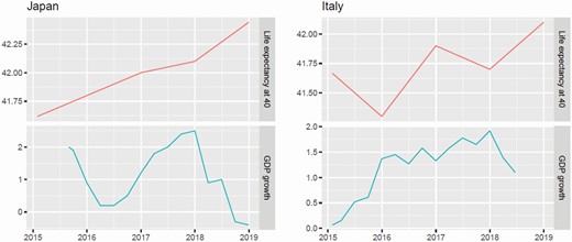
GDP Growth and Life Expectancy at 40 for Japan and Italy, 2015–2018.
Lastly, the SWB indicator is positively and significantly related to Well-being in both countries. Nevertheless, the coefficient is higher in the Japan case, highlighting that SWB-J more closely resembles the well-being level, as depicted by the latent variable.
8. Discussion and Limits of the Approach
This was the first attempt to elaborate a subjective well-being index based on Twitter data for Japan. This work shows that the same approach used to construct the analogous subjective well-being indicator for Italy can be transposed to Japan. The limitation of the human supervised method is that mother-tongue coders are needed to build the training set, but once that is done, the iSA algorithm (being completely agnostic to language) works seamlessly.
The structural equation model helps emphasize the differences between Japan and Italy, particularly with regard to the relevance of objective elements and circumstances in determining perceived well-being. In fact, it seems that Japanese subjective well-being is less affected by economic conditions, suggesting that personal, relational, and familiar dimensions may play a more important role in the individual and social well-being spheres. By nature, our well-being index is closely related to public perceptions of economic conditions, but we also need to be aware that it is not identical to them. As this is an effective measure of emotional well-being, we may need to be cautious in not conflating it with a measure for economic trends, to be used for forecasting.
However, the short time series for Japan may be one of the causes of the non-significance of some coefficients. Therefore, future work is needed to collect more data in terms of volume and time, in order to test the robustness of the results we obtained. As shown in the Supplementary Appendix, the set of keywords used to select the training set data may be enlarged to encompass more variations on the same concepts. Further, as shown in the Italian case (Iacus et al. 2019, 2020a, 2020b), sub-national differences could be examined in further development and applications of the indicator. As far as the posted messages are geolocalized, in fact, the SWB-J can be evaluated at regional or district level. Unfortunately, geolocalization is not available in this dataset, preventing this extension of the research.
An application of these two Twitter-based SWB indicators to the COVID-19 pandemic has been proposed by these authors in another study. Unfortunately, the data collection was not completely successful in 2020 due to some changes to Twitter APIs and policies. Nevertheless, we could see a generalized drop of the two indexes during the first nine months of 2020. Full details of that analysis are available in Carpi et al. (2021).
Footnotes
Also known as ‘observer effect’, it is the phenomenon by which individuals modify their behavior in response to their awareness of being observed (Landsberger, 1958).
The term is a contraction for ‘now’ and ‘forecasting’: it refers to the opportunity to collect information about some quantities or variables in real time.
For example, in a tv political debate, any non-electoral mention to the candidates or parties are considered as D0, or pure Off-Topic texts like spamming, advertising, etc.
By pre-processing phase, we mean all the textual data cleaning operations including: removal of stop words, punctuation, very frequent words (like conjunctions, prepositions, etc), numbers, special characters (#, @, etc.), and the reduction of words into stems, unigrams, etc.
In fact, despite several positive spikes, the average SWB-I in 2015 is the lowest of the examined period.
It is worth noting that the correlation coefficients among nonlinear time series are usually lower than those in standard linear models.
References
Author notes
The data collection was performed with the Japan Science and Technology Agency CREST (Core Research for Evolutional Science and Technology) project, grant n. JPMJCR14D7. This work was also performed in collaboration with the Waseda Institute of Social Media Data (WISDOM), especially the human coding of the training set. We thank Jiji Press for making their monthly polls data available and Hanako Ohmura for her valuable support.
