Socioeconomic Disparities in Parental Spending after Universal Cash Transfers: The Case of the Alaska Dividend

Abstract

Parental child-related spending represents an important pathway to promote children’s human capital development and material well-being. It is also, however, a pathway that perpetuates social inequalities given the well-known socioeconomic divide in parental spending on children. Although several studies have documented the extent to which current family income is associated with spending on children, we still know little about the causal effects of additional income on child-related spending across the socioeconomic strata. In this paper, I examine the effects of income gains due to universal and unconditional cash transfers from the Alaska Permanent Fund Dividend on child-related spending. Using longitudinal household expenditure data from the 1996–2015 Consumer Expenditure Surveys, I exploit exogenous variation in the generosity of the Alaska Dividend to estimate short- and long-term disparities in parental expenditures resulting from payouts. Results provide a unique opportunity to compare the behavior of high- and low-income parents after an income boost. I find that low- and middle-income parents use cash transfers to catch up with their more affluent counterparts in the short and long term. Low-income parents are, however, unable to keep up with the long-term increases in child-related spending made by their middle-income counterparts. Implications of results for the reproduction of socioeconomic inequalities and for current and proposed cash-transfer policies are discussed.

Introduction

Parental expenditures represent an important pathway to promote child well-being since financial resources may be used to purchase goods that improve children’s material experiences such as clothes, and computers, or goods that shape children’s life chances, including stimulating home environments, high-quality neighborhoods, and enriching extracurricular experiences (Downey, von Hippel, and Broh 2004; Potter and Roksa 2013; Waldfogel and Washbrook 2011). It is also, however, a pathway that may perpetuate social inequalities given the well-known socioeconomic divide in parental spending on enrichment items and experiences, including books, lessons, and trips, and on consumer goods, including clothing and electronics (Duncan, Magnuson, and Votruba-Drzal 2014; Gregg, Waldfogel, and Washbrook 2006; Kaushal, Magnuson, and Waldfogel 2011; Kornrich and Furstenberg 2013). Although several studies have documented the extent to which current income is associated with spending on children, we still know little about the causal effects of income increases on child-related spending across the socioeconomic strata (Kaushal, Magnuson, and Waldfogel 2011).

Establishing the effects of income gains on parental spending is challenging because family income is deeply intertwined with other forms of individual, social, and institutional inequalities. To do this in a persuasive manner, we need to examine budget variations that are independent from family characteristics such as exogenous income variation caused by government cash-transfer programs. Although a handful of studies have investigated the effects of government cash-transfer programs on child-related spending among low-income families (Gregg, Harkness, and Machin 1999; Gregg, Waldfogel, and Washbrook 2005, 2006; Jones, Milligan, and Stabile 2019), there is still a dearth of evidence on the effects of cash transfers for a broader set of families.

In this paper, I examine the effects of cash transfers that parents receive from the Alaska Permanent Fund Dividend (henceforth Alaska Dividend), which is the only universal and unconditional cash-transfer program in the western industrialized world (Widerquist and Howard 2012). The Alaska Dividend distributes equal cash payments to all Alaskans regardless of income, benefitting parents over the whole socioeconomic spectrum. As a result, this program provides a unique opportunity to investigate differences in the effects of income gains between parents of high and low socioeconomic statuses. As income rises for all, which families spend more on goods and services that contribute to children’s development and material well-being?

Using longitudinal household expenditure data from the Consumer Expenditure Surveys, I exploit exogenous variation in the generosity of Alaska Dividend’s payouts to estimate short- and long-term disparities in parental expenditures around the time of Dividend receipt. I focus on parental spending on a bundle of goods that promote children’s learning and development, such as spending on educational institutions, recreational activities, and extracurricular lessons; I also measure, however, spending on consumer goods targeted at children such as clothes and electronics (i.e., videogames, computers). I find that low- and middle-income parents use cash transfers to catch up with their more affluent counterparts in the short and long term. Low-income parents are, however, unable to keep up with the long-term increases in child-related spending made by their middle-income counterparts. These results contradict current policy discourses implying that lower-income parents cannot be trusted to spend cash transfers in ways that benefit children (Danziger 2010; Shaefer and Edin 2013) while simultaneously suggesting the limitations of universal cash-transfer policies to mitigate existing inequalities.

Background

Socioeconomic Differences in Spending on Children

Parents use financial resources to purchase a bundle of goods that shape children’s life chances, including stimulating home environments, high-quality neighborhoods and institutions, and enriching extracurricular experiences (Blau and Duncan 1967; Bourdieu and Passeron 1990; Coleman 1988; Jencks 1972). These expenditures, however, vary by social class (Brooks-Gunn, Duncan, and Britto 1999; Duncan, Magnuson, and Votruba-Drzal 2014). Early sociological research identified socioeconomic gaps in participation in “high-brow” cultural activities like museum or concert attendance (Bourdieu 1984; DiMaggio 1982). Recently, studies found that these socioeconomic gaps also occur in terms of expenditures on higher-quality educational institutions and daycares, after-school and summer programs, and enrichment items and experiences such as books, toys, games, computers, lessons, and trips (Bainbridge et al. 2005; Bradley et al. 2001; Danziger and Waldfogel 2000; Lareau 2011; Mauldin, Mimura, and Lino 2001). This spending divide may represent an important factor in the perpetuation of social inequalities given that it is driven by spending in services and goods that promote children’s human capital development and prepare them for success in college and in the labor force (Doepke and Zilibotti 2019; Lareau 2011; Potter and Roksa 2013; Schneider, Hastings, and LaBriola 2018; Waldfogel and Washbrook 2011).

Socioeconomic disparities in parental spending, however, are not restricted to spending that promotes children’s achievement, learning, and development. Previous studies have also documented socioeconomic disparities in spending that shapes children’s material well-being, such as spending on children’s clothing or electronics (Bianchi et al. 2004; Kaushal, Magnuson, and Waldfogel 2011; Kornrich and Furstenberg 2013; Ziol-Guest 2009), as well as the impacts of cash transfers on the purchase of these consumer goods (Gregg, Waldfogel, and Washbrook 2005; Halpern-Meekin et al. 2015; Jones, Milligan, and Stabile 2019; Tach et al. 2019). Often, these consumer goods are seen as investments in the material well-being of children that are not clearly associated with learning, development, and attainment (Gregg, Waldfogel, and Washbrook 2006; Schneider, Hastings, and LaBriola 2018). Still, an argument has also been made that spending on clothing or electronics may grant cultural capital and help children develop class-appropriate tastes (Kaushal, Magnuson, and Waldfogel 2011; Kornrich and Furstenberg 2013) and some empirical evidence suggests that investments in some types of electronics, such as computers, can enrich children’s home learning environment and improve their cognitive skills and academic performance (Malamud and Pop-Eleches 2011; Shields and Behrman 2000; Subrahmanyam et al. 2000).

There are several reasons for the existence of a socioeconomic divide in child-related spending that promotes human capital development or material well-being. Models of household economics suggest that access to economic resources is one of the strongest determinants of parental spending on children and that the existing gap in spending is mostly shaped by the material constraints facing low-income parents (Becker 1993; Bennett, Lutz, and Jayaram 2012; Chin and Phillips 2004). In other words, children in low-income families are disadvantaged because their parents have fewer financial resources to invest in them (Becker 1993; Danziger and Waldfogel 2000; Kalil and Deleire 2004). Parental spending on children, however, is likely not only a function of economic resources but also of cultural differences and structural opportunities that vary along socioeconomic lines (Calarco 2014; Schneider, Hastings, and LaBriola 2018). For instance, the “concerted cultivation” parenting style of the middle and upper classes imply that advantaged parents disproportionately value spending on structured activities and educational institutions as a way to transmit social and cultural capital to children (Chin and Phillips 2004; Lareau 2011). As a result of these material, cultural, and structural differences, universal income increases may yield substantial socioeconomic inequalities in subsequent child-related spending patterns. Unfortunately, we still do not know much about how the spending behavior of parents across the socioeconomic strata varies after income boosts.

Only a few studies have looked at how exogenous changes to income resulting from cash transfers affect patterns of child-related spending, most of them focusing on low-income families. In the context of the United States, low-income families in the New Hope antipoverty experiment used their additional income to spend on childcare, after-school activities, and other enrichment programs (Duncan, Huston, and Weisner 2007). Studies of Earned Income Tax Credit (EITC) beneficiaries also found that low-income working parents increase spending on childcare, enrichment items for children, and after-school activities, but also on consumer goods such as clothing after payouts (Halpern-Meekin et al. 2015; Tach et al. 2019). In Canada, low-income families who received the National Child Benefit increased their spending both on school tuition and childcare, as well as on electronics such as computers (Jones, Milligan, and Stabile 2019). Analyses of antipoverty reforms in the United Kingdom found that low-income families were able to narrow the socioeconomic spending gap by disproportionately allocating payouts to goods and services targeted at children, such as toys, books, games, and computers (Gregg, Waldfogel, and Washbrook 2005). Although studies focusing on conditional or means-tested cash-transfer programs provide a portrait of the effects of income on child-related spending among low-income families, they are limited in their ability to compare families over a broad range of incomes.

To date, theory and empirical research remain unclear on the heterogeneous effects of universal payouts—equal payouts to all regardless of age, race, sex, work status, or income. Universal payouts may mitigate the existing income gap in spending if low-income families shift away from bare necessities or dedicate a greater portion of their income to children in an effort to “catch up” with their affluent counterparts (Gregg, Waldfogel, and Washbrook 2006; Kornrich and Furstenberg 2013). The spending divide could also decrease if some child expenses are substantially less elastic among families in the top income quintile (Kaushal, Magnuson, and Waldfogel 2011) who may have already reached a “ceiling” for certain expenditures.

On the other hand, the existing socioeconomic gap in child-related spending may be exacerbated if advantaged families disproportionally prioritize financial investments in children’s learning and development compared to their disadvantaged counterparts (Calarco 2014; Cheadle and Amato 2011; Lareau 2011). The spending divide may also increase if advantaged families have more structural opportunities to enact child-related spending—such as access to cultural centers, sporting facilities, or flexible work schedules (Chin and Phillips 2004; Rosier 2000; Rosier and Corsaro 1993). Finally, although universal and equal cash transfers would represent a greater proportion of the income of disadvantaged families, these families may need to dedicate a larger share of the payouts to address unmet basic needs (Halpern-Meekin et al. 2015; Tach et al. 2019). If a greater portion of the payouts is perceived as disposable income by high-income families, we may see greater increases in child spending among this group. Although the present study is unable to conclusively discern the cultural, structural, or institutional causes of socioeconomic disparities in spending, it advances the literature by describing how parents’ spending behaviors vary along socioeconomic lines after income boosts.

The Case Study: The Alaska Permanent Fund Dividend

The Alaska Permanent Fund, a sovereign wealth fund, was established when oil production began in the state in 1976. Ever since, one-quarter of oil royalties have been dedicated to the Permanent Fund, in addition to any appropriations made by the legislature as well as inflation-proofing deposits. Starting in 1982, a portion of the annual dividend income from the Permanent Fund has been distributed to all Alaskan residents on a yearly basis in the form of the Alaska Permanent Fund Dividend. Specifically, 10.5% of the Permanent Fund’s realized net income for the past five fiscal years is dedicated to the Dividend. This formula has remained constant over the life of the program, as it was designated as a smoothing mechanism¹ and ensures that dividends are not interrupted in years when the fund loses money or investments (Erickson and Croh 2012; Widerquist and Howard 2012).

The Alaska Permanent Fund Dividend is a universal, individual, anticipated, and large cash transfer. First, it is universal and individual because all Alaskan residents who have been living in the state for at least one year, regardless of age or income, are eligible to receive the same Dividend payout. Second, it is anticipated because recipients know when they are going to receive the payout (in October of each year), and they know how much money they are expected to receive (the formula to calculate the payout is widely publicized). Finally, the payouts are large: A resident of Alaska between 1982 and 2010 would have received 29 dividends totaling $32,191 in 2010 dollars (Erickson and Croh 2012). Figure 1 displays the adjusted individual payout from the Dividend as well as take-up rates (proportion of people in Alaska who receive the Dividend) for the period covered in this study. It reports on the wide variability of individual payouts and high uptake over time.

Figure 1

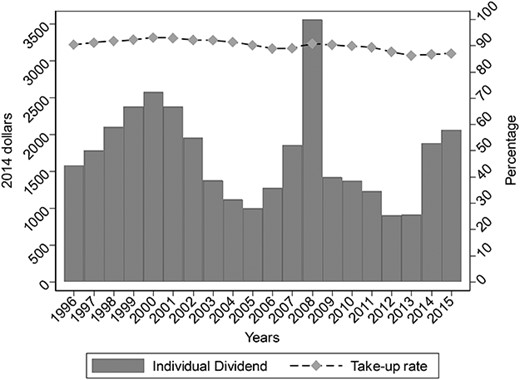
Alaska Permanent Fund Dividend payout (in 2014 dollars) and take-up rates by year.

Although combating poverty was not its original goal, the Alaska Dividend, along with safety net programs by the federal government and regional Native American corporation dividends (Berman 2018), has been credited with reducing the levels of poverty in Alaska. After all, it has provided unconditional assistance to needy Alaskans at a time when most states have scaled back aid and increased conditionality (Widerquist and Howard 2012). Not surprisingly, the Dividend has become particularly important for Alaskans who do not qualify for federal assistance programs, such as single men without work history, women who exhausted TANF eligibility, and some seniors (Berman 2018).

Despite alleviating poverty via an income effect, the Dividend has also been found to increase income inequality in Alaska in the short and long run (Kozminski and Baek 2017). Increases in income inequality due to the payouts likely result from differences in the consumption patterns of low- and high-income families who receive the payout (Kozminski and Baek 2017). For example, whereas lower-income Alaskan families may spend the payouts on nondurable goods such as winter coats, higher-income families may invest the payouts in long-term growth investments, such as their homes or 401(k)s (Widerquist and Howard 2012).

Unfortunately, only two studies have investigated consumption patterns resulting from the Dividend payouts so far (Hsieh 2003; Kueng 2018). The most recent study (Kueng 2018) used transaction data to show that Alaskans spend significantly more than non-Alaskans in the three months after payouts, with most of the spending happening immediately after payouts are disbursed, in October. Specifically, Kueng (2018) finds a marginal propensity to consume on small durables (clothes, electronics) of 8% in October and of 13% in the quarter following payouts. Although economic theory and empirical evidence suggest that spending on durable goods is likely to be timed to the arrival of large and predictable payouts (Mian and Sufi 2012; Baker, Johson, and Kueng 2017), Kueng (2018) also finds a significant and large marginal propensity to consume on nondurables (e.g., recreation) resulting from the Dividend: of 12% in October and of 25% in the quarter following payouts. These results are aligned with several studies of consumption after lump-sum payments, such as stimulus payments (for review, see Jappelli and Pistaferri 2010).

Surprisingly, the marginal propensity to consume on nondurables due to the Alaska Dividend is greatest among higher-income families (MPC = 50%), who also have higher levels of liquidity. In other words, lower-income households smooth spending on nondurables more than higher-income households. Kueng (2018) speculates that this finding results from perceptions of the Dividend as a windfall, which richer households would be more likely to squander without guilt, or from social norms that promote lavish spending among affluent families during the disbursement period. Although Kueng’s (2018) results highlight socioeconomic differences in spending decisions after universal cash transfers, his work did not specifically investigate spending on children.² The present study addresses this gap by investigating the effects of the Alaska Dividend payouts on child-related spending across the socioeconomic spectrum. Notably, spending on children may be more responsive to payouts than other kinds of spending due to a labeling effect (Thaler 1999; Kooreman 2000; Zelizer 2017).

The Present Study

This study investigates whether income gains due to universal cash transfers impact child-related spending behaviors and whether this impact varies by parents’ income level: As income rises for all, which families spend more on goods and services that contribute to children’s development and material well-being? To answer this question, I investigate socioeconomic disparities in both short-term spending behaviors (spending around the time of payout receipt) and long-term spending behaviors (spending behaviors over the course of a year). I promote a more complete understanding of the composition of child-related spending, by investigating whether universal cash transfers are allocated to spending categories that represent investments in bare necessities (clothes), big ticket items (electronics), or human/cultural capital development (e.g., education, childcare, enrichment, recreation). By revealing how much parents spend on their children when they receive a cash transfer, and what types of expenditures they prioritize, this analysis adds to our understanding of the drivers of expenditure decisions and the mechanisms by which parental income can enhance child well-being.

Method

Data

I use data from the 1996–2015 waves of the Consumer Expenditure Survey (CEX), which provides information on the spending of American consumers. Every year, the CEX fields a new panel of the survey and interviews households five times. The first interview collects baseline information. The second through fifth interviews are conducted quarterly (three months apart) and solicit detailed information on expenditures that occurred in the three months prior to each interview. In the absence of attrition, this yields 12 months of detailed monthly expenditure information.

The initial sample was composed of 182,430 households for which data were collected between the start of 1996 and the end of the first quarter of 2015. I excluded household quarters that did not have at least one child under 18 (65% of all household quarters) and further excluded households that did not have information on state of residence (12% of remaining household-quarters).³ To avoid outliers, I also exclude extremely large households (more than 7 people). The final analytic sample was composed of 52,325 households (911 Alaskan households and 51,414 non-Alaskan households) and 445,932 household months. Both Alaskan and non-Alaskan households were observed for about 8.4 months on average.

Measures

Child expenditures per resident child

Following previous literature (Gregg, Waldfogel, and Washbrook 2005; Kaushal, Magnuson, and Waldfogel 2011; Kornrich and Furstenberg 2013), I define three categories of spending on nondurable goods that represent investments in children’s learning and development: (1) educational institutions⁴ (transportation, tuition, fees, school books, and other supplies for daycares, preschool programs, elementary, middle, and high school), (2) extracurricular lessons (participation in sports, recreational lessons, tutoring services), (3) recreation (movies, theater, sporting events, toys, games, crafts). Also following previous studies (Bianchi et al. 2004; Kaushal, Magnuson, and Waldfogel 2011; Kornrich and Furstenberg 2013; Ziol-Guest 2009), I include two categories of durable goods that improve children’s material well-being: (4) children’s clothes and equipment for infants and (5) electronics (e.g., computers for non-business use, videogames). Household expenses on these five items are adjusted to 2014 dollars using the PCE-PI inflation adjustment series and divided by the number of resident children under 18 to produce a measure of spending per child. For each child-related expenditure category, I drop the top one percent of expenditures to avoid unduly influential outliers (see also Schneider, Hastings, and LaBriola 2018).⁵

Family Dividend payout

The annual individual Dividend payout’s amount, which is the same for every Alaskan resident, is publicly available (see figure 1) and was adjusted to 2014 dollars using the PCE-PI inflation adjustment series. The Dividend payout received by each Alaskan family was imputed by multiplying the individual Dividend payout by family size. Although previous literature suggests that the effects of the Dividend are concentrated in and around the month of the payout (Kueng 2018), I allow the dividend’s effect to spill over into the following calendar year. Specifically, I assign the payout from October of one year to the six months prior and following the payout. For example, the payout from October of 2010 is assigned to the months between April of 2010 (t − 6) and March of 2011 (t + 6).⁶

Family permanent income

Following previous literature (Archibald and Gillingham 1981; Deaton and Muellbauer 1980; Kaushal, Magnuson, and Waldfogel 2011; Kueng 2018), I use the annualized sum of all expenses incurred by a family in the period in which it is observed as a proxy for family permanent income (Fisher, Johnson, and Smeeding 2013; Friedman 1957). This measure is preferred over family’s current income because reported income suffers from substantial measurement error in the CEX, which attenuates the estimated spending response (Kueng 2018).⁷ Family permanent income was also adjusted to 2014 dollars using PCE-PI inflation adjustment.

Individual dividend generosity

In between-household models (described below), I use measures of individual payout generosity. I created three groups that indicated levels of generosity of individual payouts in the period in which families are observed: (1) low levels of generosity (less than $1,200), (ii) mid-levels of generosity ($1,201–1,999), and (iii) high levels of generosity (over $2,000). Results are robust to how assignment of Dividend generosity groups is made (using terciles, quartiles, or quintiles of individual payout).

Family’s income rank

Because this paper focuses on alleviation of material constraints, socioeconomic status is measured using families’ permanent income. I create percentiles of family’s permanent income within the CEX data for each year and classify households as falling into the 25th percentile and below, between the 26th and 75th percentiles, and above the 76th percentile. Results are robust to how assignment of income-rank groups is made (below 33rd, 34th–66th, and above 67th; or below 25th, 26th–50th, 51st–75th, above 76th). The chosen measure is on par with much of the literature investigating socioeconomic gaps in spending on children, which has found that the top one or two deciles stand in stark contrast with other income groups (Kornrich 2016; Kornrich and Furstenberg 2013; Schneider, Hastings, and LaBriola 2018). Analyses investigating spending patterns of families above the 90th percentile separately are hindered due to small sample sizes of Alaskans households in that group but corroborate main results (results available upon request).

Controls

Multivariate analyses include controls for reference parent’s characteristics (gender, age, age squared, race,⁸ educational attainment, marital status, working status, occupation industry) and family characteristics (family structure, family size, number of children, age composition of resident children, and family’s permanent income).

Following previous literature, some of the main results compare Alaskan families to other US families (Hsieh 2003; Kueng 2018). Table 1 indicates some substantively small differences between Alaskan and other US households: Alaskan heads are more likely to be educated (percentage with college degree: 33% vs. 29.%), to work full time (75% vs. 68%), to be married (71% vs. 70%), and to have younger children (percentage with children under age six: 25% vs. 23%). Although Alaskans and other Americans are similarly likely to be White (77% vs. 76.7%), Alaskans are substantially more likely to be a non-Black racial minority (17% vs. 6%).

Table 1

Descriptive Statistics Benchmarked

	CEX		ACS/Census
	United States	Alaska	United States	Alaska	Anchorage
	(1)	(2)	(3)	(4)	(5)
Head’s characteristics
Male	0.457	0.459	0.413	0.435	0.416
Age	39.1	39.3	37.92	38.17	38.11
Race
White	0.767	0.770	0.784	0.729	0.741
Black	0.169	0.064	0.152	0.047	0.086
Other	0.064	0.166	0.064	0.223	0.173
Education
High school or less	0.404	0.320	0.478	0.457	0.379
Some college	0.305	0.355	0.247	0.296	0.312
College or more	0.292	0.325	0.275	0.246	0.310
Marital status
Married	0.697	0.705	0.664	0.668	0.654
Widowed/Separated	0.177	0.199	0.175	0.183	0.178
Never married	0.126	0.096	0.161	0.149	0.168
Work status
Works less than 20 hours/week	0.050	0.039	0.039	0.045	0.042
Works 20–36 hours/week	0.096	0.080	0.151	0.151	0.143
Works 37+ hours/week	0.678	0.750	0.641	0.666	0.686
Not working	0.175	0.125	0.169	0.138	0.130
Family characteristics
Family structure
Husband, wife, and kids	0.611	0.615	—	—	—
Single parent	0.200	0.207	—	—	—
Other family structure	0.189	0.178	—	—	—
Family size	3.9	3.7	4.0	4.1	4.0
Number of kids	1.8	1.7	1.9	2.0	1.9
Oldest child’s age
Less than 6	0.233	0.251	0.232	0.228	0.251
6–11	0.257	0.250	0.292	0.276	0.275
12+	0.510	0.498	0.476	0.496	0.474
Family permanent income (in 2014 dollars)	57,494	59,930	—	—	—
Household dividend (in 2014 dollars)	0	4,604	—	—	—
N	51,414	911	4,479,610	14,688	2,096

Sources: Consumer Expenditure Survey (1996–2015); American Community Survey (2001–2015); Census (1990, 2000).

Table 1 also benchmarks the CEX data using data from the Census and American Community Surveys (ACS). Overall, Alaskans in the CEX sample are more socioeconomically advantaged than those in the Census/ACS sample. This results from the fact that the CEX does not collect data to be representative at the state level, with data collection efforts in Alaska being concentrated on Anchorage. Not surprisingly, Table 1 indicates that the CEX sample is more representative of Anchorage county than of the state of Alaska as a whole. Although the CEX data cannot inform on the spending patterns of all Alaskans, this study’s goal is to compare a group of Americans who receive unconditional cash transfers to Americans who do not. A sample that is representative of Anchorage better serves this purpose, given that rural Alaska tends to be more remote than rural areas in the rest of the US. Sensitivity analyses (available upon request) including adjusted weights to ensure representativeness on the observed characteristics yielded the same results.

Empirical Strategy

Short-term models

I exploit the seasonal and lump-sum nature of the Dividend payouts as well as the continuous monthly sampling frame of the CEX to investigate changes in spending around the time of benefit receipt. This identification strategy is akin to a difference-in-difference and relies on a comparison of monthly patterns of Alaskan households’ spending to that of other US households to identify whether child-related expenditures of Alaskan households increase disproportionally more than that of other US households in the months surrounding benefit payout. Exploiting the exogenous timing of payout disbursement has been a common strategy to address endogeneity and identify the effects of economic stimulus payments, tax rebates, and tax credits on consumption (Agarwal, Liu, and Souleles 2007; Barrow and McGranahan 2000; Johnson, Parker, and Souleles 2006; Kueng 2018; Parker et al. 2008).

This identification strategy assumes that all other US states provide the appropriate counterfactual of the spending trends that we would see among Alaskan households in the absence of payouts. Appendix Table A in the Online Appendix supports this assumption by providing evidence that the seasonality of spending patterns in all categories of expenses between Alaskan families and other US families is similar. A related assumption made in this paper is that there are no reasons other than the payouts itself why Alaskans would increase their spending around the time benefits are paid relative to other US households. A final important assumption made in this study is that the timing of treatment (payouts) is independent from the outcomes of interest (spending on children). Although this assumption cannot be tested, a few facts suggest that it is also met: 1) decisions about the timing of the intervention were not shaped by patterns of child-related spending during the inception of the Alaska Dividend program; 2) the timing of disbursement has been fixed since 1982, being unresponsive to patterns of child-related spending; 3) previous analyses suggest that there is little to no anticipatory effects of the payouts on spending (Kueng 2018).

I measure changes in child-related spending in relative terms using log-linear models.⁹ These models capture relative increases in spending resulting from a relative increase in income due to the Alaska Dividend. Thus, they consider not only how much was received and how much was spent but also how payouts compare to families’ income and how increases in spending compare to families’ baseline spending. This choice is important for a few reasons: (1) It acknowledges that low-income parents may increase spending relatively more than higher-income parents even if they spend a lower amount of dollars on children compared to their affluent counterparts; (2) it keeps my models in line with the two previous studies using the CEX to investigate the impacts of the Alaska Dividend on spending (Hsieh 2003; Kueng 2018); (iii) it addresses positive skewedness in expenditures variables through log-transformation and yields normally distributed residuals.

$$\begin{align} \ln\;\left({C}_{i\theta t}\right)=a+\gamma{T}_{i t}+\sum \limits_{\theta }{\delta}_{\theta }{M}_{i\theta}+\sum \limits_{\theta }{\beta}_{\theta}\left({T}_{i t}\times{M}_{i\theta}\right)+{x}_{i\theta t}\lambda +{\varepsilon}_{i\theta t} \end{align}$$

(1)

$$\begin{align} {\displaystyle \begin{array}{l}\ln \left({C}_{i\theta t}\right)=a+\gamma{T}_{i t}+\sum \limits_{\omega }{\phi}_{\omega }{I}_{i\omega}+\sum \limits_{\theta }{\delta}_{\theta }{M}_{i\theta}+\sum \limits_{\omega }{\psi}_{\omega}\left({T}_{i t}\times{I}_{i\omega}\right)\\{}\kern2.16em+\sum \limits_{\theta }{\eta}_{\theta}\left({T}_{i t}\times{M}_{i\theta}\right)+\sum \limits_{\sigma }{\varphi}_{\sigma}\left({I}_{\omega}\times{M}_{i\theta}\right)\\{}\kern2.16em +\sum \limits_{\sigma }{\beta}_{\sigma}\left({T}_{i t}\times{I}_{i\omega}\times{M}_{i\theta}\right)+{x}_{i\theta t}\lambda +{\varepsilon}_{i\theta t}\end{array}} \end{align}$$

(2)

where C_iθt indicates deviations from household average spending per resident child in month θ and PFD year t (from April to March). To create an estimate that is akin to income elasticity, T_it denotes the family Dividend payout normalized by family permanent income and multiplied by 100, and M_iθ represents a series of indicators for the months household i is observed, with October omitted as a reference category. The coefficients on the interactions between T_it and M_iθ (β_θ) describe how patterns of expenditures for Alaskan households differ from non-Alaskan households in a particular month, controlling for overall differences in expenditures between Alaskan and non-Alaskan households over the course of a year. The key coefficients of interest come from the interactions between the October month indicator and the T_it indicator (⁠|$\hat{\beta}$|_Oct), as well as surrounding months. Significant coefficients on these interactions indicate that Alaskan households change their expenditure patterns in October in ways that are significantly different than non-Alaskan households. These coefficients identify whether a percentage point increase in the share of Alaskan families’ permanent income that is represented by payouts leads to a percent change in monthly child-related spending relative to non-Alaskan households. x_iθt is the time variant 1 × k regressor vector (where k is the number of socioeconomic and demographic controls as well as state, calendar year, family size, and number of children fixed effects) and λ is the k × 1 vector of parameters. ε_iθt are changes in spending not explained by either the Dividend or the controls. Whereas Eq. (1) is used to estimate average marginal effects for the whole sample, Eq. (2) estimates socioeconomic differences in the effects of the Dividend payout by including I_iω, which represents indicators for families’ income-rank, where ω θ ϵ {≤25th, 26th to 75th, ≥76th percentiles}. All panel analyses are weighted and use robust standard errors clustered at the household level.¹⁰

Long-term models

The models specified in Eqs (1) and (2) above are well suited to capture parents’ spending decisions and behaviors in the months immediately surrounding a cash transfer, when disposable income increases. Coupling spending increases with the exogenous timing of disbursement also provides stronger evidence of the causal link between the payouts and subsequent expenditures. This strategy, however, cannot identify aggregate increases in child-related spending due to unconditional cash-transfers (i.e., absolute increases that are independent of timing). Identifying aggregate effects is particularly important because short-term responses may vary because of socioeconomic differences in credit constraints. Research suggests that whereas lower-income households more often spend their cash transfers quickly, higher-income households are more likely to smooth their spending by saving or paying down debt (Agarwal, Liu, and Souleles 2007; Bertrand and Morse 2009; Cole, Thompson, and Tufano 2008; Johnson, Parker, and Souleles 2006).

I conduct a second set of analyses that compare the annualized¹¹ spending of Alaskan and non-Alaskan households in periods of high versus low payout generosity, averaging levels of Dividend income and spending over several years. I use the following between-household ordinary least squares model with robust standard errors:

$$\begin{align} \ln \left({A}_i\right)=a\sum \limits_{\theta }{\gamma}_{\theta }{G}_{i\theta}+\eta A{K}_i+\sum \limits_{\theta }{\beta}_{\theta}\left({G}_{i\theta}\times A{K}_i\right)+{x}_i\lambda +{\varepsilon}_i \end{align}$$

(3)

$$\begin{align} {\displaystyle \begin{array}{l}\ln \left({A}_i\right)=a+\sum \limits_{\theta }{\gamma}_{\theta }{G}_{i\theta}+\eta A{K}_i+\sum \limits_{\omega }{\phi}_{\omega }{I}_{i\omega}+\sum \limits_{\theta }{\delta}_{\theta}\left({G}_{i\theta}\times A{K}_i\right)\\{}\kern1.8em+\sum \limits_{\omega }{\psi}_{\omega}\left({I}_{i\omega}\times A{K}_i\right)+\sum \limits_{\pi }{\varphi}_{\pi}\left({G}_{i\theta}\times{I}_{i\omega}\right)\\{}\kern1.8em +\sum \limits_{\pi }{\beta}_{\pi}\left({G}_{i\theta}\times{I}_{i\omega}\times A{K}_i\right)+{x}_i\lambda +{\varepsilon}_i\end{array}} \end{align}$$

(4)

where A_i represents annualized spending per resident child by household i and G_iθ represents indicators of individual payout generosity for the year in which a family is observed, where θ ϵ {≤$1,200, $1,201 to $1,999, ≥$2,000)}. AK_i is a dummy variable that indicates Alaska residence. Models include year and family size fixed effects, all socioeconomic and demographic controls described above (x_i) averaged, as well as additional dummies for seasons in which a household was observed before expenses were annualized. Whereas Eq. (3) is used to estimate average marginal effects for the whole sample, Eq. (4) estimates socioeconomic differences in the effects of the Dividend payout by including I_iω, which represents indicators for families’ income rank, where ω ϵ {≤25th, 26th to 75th, ≥76th percentiles}.

Robustness checks

For both short-term and long-term models, I tested whether results are sensitive to alternative variable transformations (Inverse Hyperbolic Sine), model specifications (Poisson models; Logistic models), sample restrictions (households who provided complete information on 12 months of expenditures), and control groups (Northwestern states only). I have also estimated Marginal Propensities to Consume using linear models and two-part models. These robustness checks are described in detail in the Online Appendix and highlighted in the discussion of results whenever they do not corroborate the main findings presented in this paper.

Results

Spending on Children Immediately after Universal Cash Transfers

Figure 2 reports on the average marginal effects of the Dividend on each category of child-related expense. Results indicate that spending on durables (electronics, clothes) is responsive to payouts, but not spending on nondurables (recreation, lessons, and education). Specifically, a one percentage point increase in the share of family’s permanent income due to the Dividend yields an increase of 8.5% in spending on clothing and a 3.7% increase in spending on electronics in October. Notably, these are substantively small increases in spending on a baseline spending per child of $25 on clothes and $26 on electronics in the average month. Furthermore, although the effects of payouts on spending on clothing are robust to alternative model specifications, effects on spending on electronics are not (see Online Appendix).

Figure 2

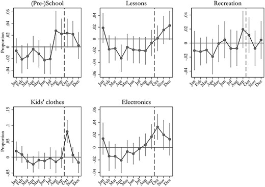
Average marginal effects of the Dividend payout on spending elasticity by spending category (Alaska versus other US States). Source: Consumer Expenditure Survey (1996–2015).

The next set of analyses assesses the responsiveness of child-related spending along income-rank lines. Table 2 shows the marginal effects of the payout on each type of expense in the last four months of the year by families’ income rank. All parents significantly increase spending on children’s clothing around the time of payout disbursement. For every one percentage point increase in the share of family’s permanent income due to the Dividend, low-, middle-, and high-income families increase their spending on clothes in October by about 5.3%, 11.6%, and 12.2%, respectively. Low- and middle-income families also significantly increase their spending in October on electronics by 2.6% and 5% and on educational institutions by about 3% (in September) and 5.6% (in October), respectively. Overall, results suggest that short-term increases in child-related spending are driven mostly by spending on clothes, electronics, and education among low-income and middle-income families and by spending on clothes among high-income families. Sensitivity analyses presented in the Online Appendix suggest that increases in spending on clothing among all income-rank groups and increases in spending on education among low-income parents are robust to alternative model specifications.

Table 2

Average Marginal Effects of the Dividend Payout on Spending (Alaska versus Other US states), by Types of Expenditures and Parents’ Income Rank

	Clothes	Electronics	Recreation	Lessons	(Pre-)School
Low income
September	−0.012	0.015	−0.002	−0.018	0.029*
	(0.018)	(0.014)	(0.013)	(0.012)	(0.013)
October	0.051**	0.026*	0.011	−0.016	0.007
	(0.019)	(0.012)	(0.014)	(0.012)	(0.012)
November	−0.018	0.015	−0.021	0.006	0.022
	(0.012)	(0.018)	(0.015)	(0.015)	(0.016)
December	0.004	0.008	−0.013	0.023	−0.009
	(0.022)	(0.020)	(0.016)	(0.016)	(0.014)
Middle income
September	0.008	0.021	0.040	0.006	0.026
	(0.030)	(0.017)	(0.026)	(0.019)	(0.026)
October	0.109**	0.049*	0.010	0.015	0.055*
	(0.034)	(0.020)	(0.025)	(0.018)	(0.023)
November	0.027	0.031	0.006	0.014	0.023
	(0.023)	(0.019)	(0.023)	(0.020)	(0.019)
December	−0.051	0.036	0.004	0.004	0.016
	(0.028)	(0.019)	(0.026)	(0.022)	(0.021)
High income
September	0.0038	0.020	0.007	−0.008	−0.013
	(0.065)	(0.034)	(0.037)	(0.040)	(0.057)
October	0.115*	0.008	−0.017	0.029	−0.016
	(0.054)	(0.027)	(0.045)	(0.044)	(0.060)
November	0.064	0.021	−0.025	0.0744	0.031
	(0.081)	(0.026)	(0.063)	(0.066)	(0.059)
December	0.025	−0.034	0.082	0.116	0.028
	(0.077)	(0.032)	(0.045)	(0.066)	(0.061)
Observations	441,473	441,481	441,474	441,473	441,474

Source: Consumer Expenditure Survey (1996–2015)

Notes: Clustered standard errors in parentheses.

^***p < .05, ^**p < .01, ^*p < .001

Overall, findings align with Kueng’s (2018) by suggesting that exogenous increases to permanent income result in short-term spending on small durables, such as clothes, across income-rank groups. Whereas Kueng (2018) found that higher-income households were also more likely to spend payouts on nondurables, which he speculates may be “lavish” spending, I find that expenses on recreation or lessons do not increase among parents across the socioeconomic spectrum and that only middle-income and, particularly, low-income families’ spending on education is responsive to payouts in the short term. This last result is aligned with a series of studies suggesting that lower-income parents may use cash transfers to “catch up” with their more affluent counterparts (Gregg, Waldfogel, and Washbrook 2006; Kornrich and Furstenberg 2013).

Universal Cash Transfers and Aggregate Spending on Children

Increases in child-related expenses identified in October may not represent absolute increases in the aggregate levels of expenses but rather a shift in the timing of expenses if parents wait until the payout to buy goods and services that they would purchase regardless of the Dividend receipt, such as winter clothes. Furthermore, low levels of liquidity among economically disadvantaged families may lead to greater short-term spikes compared to advantaged counterparts who are able to smooth spending. Next, I conduct analyses that investigate whether payouts lead to increases in aggregate or long-term spending (i.e., spending that is independent of timing). Figure 3 compares logged annualized spending of Alaskan and non-Alaskan households in high versus low Dividend periods, averaging levels of Dividend income and spending over several years (see Eq. 3).

Figure 3

Effects of the Dividend payout generosity on annualized child-related spending (Alaska versus other US states). Source: Consumer Expenditure Survey (1996–2015).

Figure 3 suggests that greater individual payout generosity is associated with significant increases in aggregate spending on lessons, recreation, and clothing. Specifically, Alaskans spend 166% (EXP(0.98)-1)x100) more on lessons for children than non-Alaskans in years when individual payouts are over $2,000. On a baseline average spending of $204 per child per year, this would represent an additional spending of $339 per child per year. Alaskans also spend almost twice as much on recreation (over 90% increase) as non-Alaskans when individual payouts are greater than $1,200. On a baseline average spending of $388 per child per year, this would represent an additional spending of over $350 per child per year. Finally, Alaskans spend over 60% more than non-Alaskans on clothes when payouts are greater than $1,200. On a baseline average spending of $296 per child per year, this would represent an additional spending of over $178 per child per year. Figure 3 also suggests that Alaskans always spend more on electronics than non-Alaskans, regardless of the generosity of individual payouts.

Overall, findings indicate that Alaskan parents' aggregate spending on electronics (big-ticket items) are greater than non-Alaskan parents spending on electronics even when payouts are small. On the other hand, Alaskan parents' aggregate spending on clothes, recreation, and lessons are only greater than non-Alaskan parents' spending on these categories when payouts are larger. A comparison between findings from the long-term (figure 3) and the short-term (figure 2) models suggests that increases in spending on electronics and clothing that occur immediately after the payouts are also identified throughout the year. In other words, increases in spending on clothes and electronics in October do not simply represent a shift in the timing of expenses, but rather a real increase in the total amount spent on those categories over the course of a year. Increases in spending on recreation and lessons, however, are only identified in the long-term models, but not in the short-term models. This suggests that Alaskan parents are able to smooth spending on these goods and services over the course of the year.

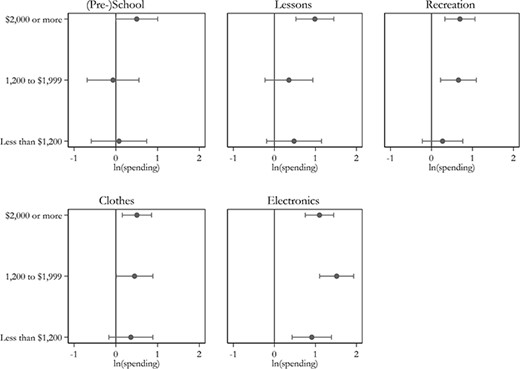
Figure 4 compares logged annualized spending of Alaskan and non-Alaskan households in periods of high versus low generosity of payouts by income-rank group, averaging income-rank specific levels of Dividend income and spending over several years (see Eq. 4). First, it indicates that greater payout generosity is only associated with increases in spending on clothes among high-income Alaskan families relative to other high-income US families. These results are aligned to short-term models and indicate that higher-income families’ short and long-term spending on other child-related spending categories is not responsive to the Dividend payout.

Figure 4

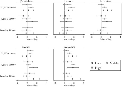
Effects of the Dividend payout generosity on annualized child-related spending (Alaska versus other US states), by parents’ income rank. Source: Consumer Expenditure Survey (1996–2015).

Second, figure 4 suggests that greater individual payout generosity is associated with increases in spending on clothes, recreation, lessons, and educational institutions among middle-income Alaskan families relative to middle-income non-Alaskan families. Middle-income Alaskan families always spend more on electronics than other middle-income American families, regardless of payout generosity. These results indicate that Alaskan middle-income families’ aggregate spending on electronics is responsive to payouts of any size, whereas spending on all other categories of spending increases as payouts become more generous. Again, a comparison between long-term (figure 4) and short-term (Table 2) models suggests that some of the increases in spending occur in the months surrounding payouts (electronics, clothing, and education) and some may be smoothed throughout the year (recreation and lessons).

Overall, among low-income families, greater individual payout generosity is associated with significant increases in aggregate spending on electronics and recreation only. Differently than middle-income families, low-income families’ aggregate spending on electronics is only significantly responsive as payouts become more generous. Like middle-income families, low-income Alaskan families likely smooth their spending on recreation throughout the year. On the other hand, short-term increases in spending on education among low-income families (see Table 2) are not reproduced on the long term, which suggests that spending on education around the time of disbursement may only represent a shift in the timing of expenses that would occur regardless of payouts. Finally (and unexpectedly), results also indicate that low-income Alaskan families spend more on clothing relative to other US families in years when payouts were less generous, but not in years when the payouts were most generous. Although these results are not robust to alternative model specifications (see Online Appendix), they may also suggest that larger payouts create opportunities for different types of investment and disincentivize investments in clothing among lower-income families.

Discussion and Conclusions

Spending on children is unequal across families, varying by parental income. This spending divide, which represents an important pathway for the reproduction of socioeconomic inequalities, has increased over time (Kornrich and Furstenberg 2013). The present study investigates socioeconomic differences in the effects of income increases due to universal cash transfers on parents’ short- and long-term spending behaviors. I use variation in the Alaskan Permanent Dividend Fund payouts to investigate whether families who receive universal cash transfers spend more on children, and whether increases in spending are moderated by parents' income-rank. Although I cannot disentangle the reasons behind the existing socioeconomic gap in spending (whether, for example, it is driven by differences in material constraints or preferences), this study advances the sociological literature and informs cash-transfer policies by providing a portrait of parents’ heterogeneous spending behaviors after universal payouts both on the short and long terms.

Immediately after receiving cash transfers, parents across the income-rank spectrum increase spending on clothing, durable goods that may improve children’s material well-being. Finding greater spending on durable goods such as clothes across income-rank groups after a lump-sum payout is in line with previous research findings (Barrow and McGranahan 2000; Johnson, Parker, and Souleles 2006; Kueng 2018). Somewhat surprising, however, spending on clothes following payouts seems to only represent a shift in the timing of this type of spending for low-income parents. In other words, even if low-income parents take advantage of the lump-sum payouts to purchase clothing, I find no evidence that they increase their aggregate spending on clothing over the course of the year as payouts increase. This finding suggests that spending on clothing may not be a priority for low-income parents or that low-income parents are unable to maintain the gains in spending on clothing made in the short term over the course of the year. Finding aggregate increases in spending on clothing among middle- and high-income parents, on the other hand, may suggest that these parents prioritize spending on clothing or that Dividend payouts allow them to better prepare for cold winters. These increases, however, may also result from what Kueng (2018) called “lavish” spending of payouts if high- and middle-income parents are spending on items that are luxury accessories rather than basic necessities. Although the CEX does not allow me to differentiate spending that is geared towards luxury or basic needs, additional analyses comparing Alaskans to Americans who live in colder northwestern states (Idaho, Montana, and Washington) also identify an effect of the Dividend on aggregate clothing expenses. I also find that increases in spending on clothing are similar for Alaskan households with young children (under 6) and with older children (over 12), despite their varied needs for purchasing clothes. Together, these two sets of results tentatively suggest that increases in spending on clothing among middle- and high-income Alaskans are not be driven by winter or basic needs.

I also find that middle- and low-income parents increase their spending on electronics both around the disbursement period and over the course of the year. Although there is no consensus on the benefits of electronics for children’s well-being and outcomes, there is incipient evidence that electronic items such as computers may help children to develop cultural and human capital (Malamud and Pop-Eleches 2011; Shields and Behrman 2000; Subrahmanyam et al. 2000). Increases in spending on big-ticket electronic items among lower-income parents who may lack access to credit or savings are not surprising. These results, however, are less robust to alternative model specifications (see Online Appendix) and should be interpreted with caution. Of policy interest, this type of spending may be at least partly promoted by the lump-sum disbursement format of the Alaska Dividend: Research conducted outside of the United States found that lump-sum transfers are more likely than continuous transfers to promote spending on durable goods and big-ticket items (Haushofer and Shapiro 2016).

In terms of investments that promote cultural and human capital development, such as investments in lessons, recreation, and education (Doepke and Zilibotti 2019; Lareau 2011; Potter and Roksa 2013; Schneider, Hastings, and LaBriola 2018; Waldfogel and Washbrook 2011), I find that parents across income-rank groups do not significantly increase their spending on recreation or lessons immediately after payouts. Although I find that low- and middle-income parents increase their aggregate spending on recreation or lessons over the course of the year (likely by smoothing spending), a lack of short-term responsiveness of spending on nondurables is in stark contrast with Kueng’s (2018) findings. Differences between studies, however, may result from differences in the population studied (i.e., increases in spending on non-durables identified by Kueng may be driven by Alaskans without children) and by greater levels of measurement error and attenuation bias in the CEX compared to the transaction data used by Kueng (2018).

In terms of spending on education, I find that only low- and middle-income parents increase their investments in education immediately after payouts, and only low-income parents’ short-term increases in spending on education are robust to alternative model specifications (see Online Appendix). These findings suggest that low- and middle-income parents use cash transfers to “catch up” with their more affluent counterparts in the short term (these results are aligned with previous studies, e.g. Gregg, Waldfogel, and Washbrook 2006; Halpern-Meekin et al. 2015; Tach et al. 2019). Findings contradict current policy discourses in the United States that often imply that lower-income parents cannot be trusted to spend cash transfers in ways that would benefit children or that lower-income parents would spend money from cash transfers in ways that are inappropriate or inherently worse than their higher-income counterparts (Danziger 2010; Shaefer and Edin 2013).

On the long term, however, low-income parents are unable to “keep up” with the increases in child-related spending made by their middle-income counterparts. Specifically, as payout generosity increases, middle-income parents increase aggregate spending on education, lessons, and recreation, but low-income parents only increase aggregate spending on recreation. In other words, the aforementioned short-term increase in spending on education among low-income parents may only represent a shift in the timing of certain educational expenses that would occur regardless of payouts. Although lower levels of long-term responsiveness of child-related spending among low-income families compared to middle-income families could result from different priorities and preferences across income groups, they may also result from differential access to structural opportunities that facilitate investments throughout the year—such as access to cultural centers, sporting facilities, or flexible work schedules (Chin and Phillips 2004; Rosier 2000; Rosier and Corsaro 1993), or from the unique material constraints faced by the most disadvantaged families. For instance, qualitative studies found that low-income parents who are beneficiaries of the EITC need to devote a large portion of EITC payouts to address unmet needs even though they consider the benefit to be the “kids’ money” (Halpern-Meekin et al. 2015; Tach et al. 2019). Corroborating this perspective, additional results [not shown] suggest that low-income parents in my sample are more likely than their middle- or high-income counterparts to increase spending on transportation maintenance, adult clothing, and utilities immediately after the Alaska Dividend payouts.

Finally, this study finds that higher-income parents’ spending on education, recreation, and lessons is unresponsive to payout receipt. This is a surprising finding given the vast literature suggesting that higher-income parents value spending in enrichment items, activities, and experiences that promote social and cultural capital (Chin and Phillips 2004; Lareau 2011). There are two ways to explain these puzzling results: First, high-income parents may have reached a “ceiling” on current spending that disincentive using additional resources on children after payouts; second, higher-income parents may be saving Dividend payouts for future use (e.g., college savings). Although this paper cannot speak to saving or debt-payment behaviors, an extensive literature in the field of economics suggests that higher-income consumers are more like to save and smooth spending after windfalls, whereas lower-income consumers are more likely to spend cash-transfers quickly (Agarwal, Liu, and Souleles 2007; Bertrand and Morse 2009; Cole, Thompson, and Tufano 2008; Johnson, Parker, and Souleles 2006). Relatedly, a prior study found that EITC recipients—who are low-income—are unable to save money from lump-sum benefits during tax time (Jones and Michelmore 2019). If higher-income parents are saving payouts to invest in children over the course of a longer period, then universal cash transfers may mitigate disparities in spending on the short-run while exacerbating these inequalities in the long-run.

This paper has important limitations. First, there are several sources of measurement error that lead to attenuation bias in the estimated effects of the Dividend: (1) spending amounts reported by respondents every three months are subject to recall bias; (ii) the Dividend receipt and amount of payout are imputed for all Alaskan households, assuming a take-up rate of 100%, and that all household members were eligible for the payout and received the payout in full; and, importantly, (iii) the Dividend is subject to federal income tax, which means that the real value of the Dividend varies by families’ income, being lower for more affluent families who pay higher marginal income tax rates on payouts. Second, the CEX data cannot determine whether expenditures were used in ways that truly enhanced children’s development and it does not allow identification of the “quality” of spending—just the dollar amount dedicated to the expenditure. Third, these data only allow me follow families for the period of one year. Significant inequalities could arise in a longer time horizon if some income groups are saving the payouts for future investments. Fourth, the child-related expenditures I consider in this paper cover only one potential mechanism by which the Alaska Dividend may enhance child well-being. Other expenditures, while not specifically child-related—such as housing, groceries, utilities, or durable goods—also benefit children. Relatedly, the benefits of the Alaska Dividend to children may not solely flow through material goods; qualitative research suggests that parents receive social psychological benefits of the refund (Halpern-Meekin et al. 2015; Sykes et al. 2015), which may indirectly benefit children via lower parenting stress and higher-quality parent-child interactions. Finally, this study provides an incomplete picture of the broader consequences of the Alaska Dividend for the reproduction of inequalities. First, the Alaska Dividend is not a redistributive policy and it has historically deviated funds from social programs that would mostly benefit lower-income Alaskan children (Widerquist and Howard 2012). Second, although Alaska lawmakers inserted a “hold harmless” provision in the 1982 legislation authorizing the use of state general funds to offset loss of certain federal means-tested benefits caused by receipt of the Dividend, take-up rates for these equivalent cash replacement payments through the State of Alaska’s Division of Public Assistance are unknown. Furthermore, although the Supplemental Nutritional Assistance Program and Supplemental Security Income program are included in the “hold harmless” provision, other programs like the EITC are not. Thus, it is possible that the additional spending incurred by lower-income families does not compensate for the potential loss in access to social services and means-tested programs that low-income children in Alaska experience. This is an important empirical question that should be addressed in future studies.

Despite these limitations, this study has important policy and theoretical implications for understanding the role of universal cash transfers in reproducing, exacerbating, or mitigating existing inequalities. Policymakers and scholars often debate how poor parents would make financial decisions when receiving cash transfers with no strings attached. Results from this study provide a unique opportunity to compare the behavior of higher- and lower-income parents after such an income boost. This work suggests that lower- and middle-income parents “catch up” with their more affluent counterparts, to varying degrees, in terms of current spending (spending during the time of disbursement or over the course of a year). Future inquiries should investigate the reasons why short- and long-term spending patterns differ as well as the potential role of saving decisions in promoting spending and consumption inequalities in the long run.

About the Author

Mariana Amorim is an assistant professor of Sociology at Washington State University and a faculty affiliate of the New York University's Cash Transfer Lab. Her research focuses on families, poverty, inequality, intergenerational support, and social policies. She holds a PhD in Policy Analysis and Management from Cornell University.

Footnotes

1

This smoothing mechanism ensures that the Dividend is not directly derived from the state’s mineral extraction revenue, which would threaten the causal estimates.

2

In a sensitivity test, Kueng (2018) investigates the spending response on specific categories of strict nondurable, including “kids’ activities” and finds very small MPC (0.007).

3

Not all states are sampled in the CEX, and some state codes are suppressed or recoded when there is a low number of respondents in a given geographic area (generally rural areas); None of the surveyed Alaska residents had their state codes suppressed between 1996 and 2015.

4

Expenses on institutional childcare and preschool are combined with expenses on school. Both types of expenses represent investments in institutional and learning environments that are available to children from infancy to the age of 18. Substantive conclusions remain the same if these categories are disaggregated.

5

Using the whole sample produces the same results.

6

In sensitivity analyses, I assigned the payout to its calendar year (from January of year t to December of year t) and to the 12 months after disbursement (October of t to September of t + 1).

7

Robustness analyses suggest that, similar to previous studies investigating the consumer response to the Alaska Dividend payout (Hsieh 2003; Kueng 2018), I find attenuated and insignificant effects when using a measure of family income instead of family permanent income in the analysis.

8

In this study, race is measured through three mutually exclusive categories: “White,” “Black,” and “Other.” Each of these categories may contain both Hispanic and non-Hispanic households. The CEX does not collect data on ethnicity before 2003, which hinders my ability to identify Hispanic families consistently in the full sample. Analyses restricting the sample to the years in which ethnicity data were collected (2003–2015) and relying on four racial/ethnic categories (Non-Hispanic White, Non-Hispanic Black, Hispanic, Non-Hispanic Other) corroborate main results and are available upon request.

9

Fixed-effects models at the household level yielded the same results.

10

Previous studies on the spending response to the Dividend (Hsieh 2003; Kueng 2018) have also clustered standard errors on the household level. Results clustering standard errors by month are less conservative than the results presented in this manuscript and are available upon request.

11

Restricting the sample to households that provided 12 months of data yields the same results.

References

Baker, Scott R., Stephanie Johnson, and Lorenz Kueng. 2017. Shopping for lower sales tax rates. No. w23665. National Bureau of Economic Research.
Bianchi, Suzanne M., Philip Cohen, Sara Raley, and Kei Nomaguchi. 2004. “Inequality in Parental Investment in Child-Rearing: Expenditures, Time, and Health.” pp. 189–220 in Social Inequality, edited by K. Neckerman. New York: Russell Sage Foundation Press.
Erickson, and Cliff Groh. 2012. “How the APF and PFD Operate: The Peculiar mechanics of Alaska's State Finances”(pp. 41#48) In Widerquist, K. and M. Howard(Eds). Alaska's Permanent Fund Dividend: Examining Its Suitability as a Model. Springer.
Jappelli, Tullio, and Luigi Pistaferri. 2010. “The consumption response to income changes.” Annu. Rev. Econ. 2(1):479–506.
Jones, Lauren E., and Katherine Michelmore. 2019. “Timing is Money: Does Lump-Sum Payment of the Earned Income Tax Credit Affect Savings and Debt?.” Economic Inquiry 57(3):1659–1674.
Kalil, Ariel, and DeLeire, Thomas. 2004. Expenditure decisions in single-parent households. In Kalil, A., and DeLeire, T. (Eds) Family Investments in Children's Potential (pp. 181–208). Psychology Press.
Kooreman, Peter. 2000. “The labeling effect of a child benefit system.” American Economic Review 90(3):571-583.
Kornrich, Sabino. 2016. “Inequalities in parental spending on young children: 1972 to 2010.” AERA Open 2.2: 2332858416644180.
Mian, Atif, and Amir Sufi. 2012 “The effects of fiscal stimulus: Evidence from the 2009 cash for clunkers program.” The Quarterly journal of economics 127(3):1107–1142.
Sykes, Jennifer, et al. 2015. “Dignity and dreams: What the Earned Income Tax Credit (EITC) means to low-income families.” American Sociological Review 80(2):243–267.
Thaler, Richard H. 1999. “Mental accounting matters.” Journal of Behavioral decision making 12(3):183–206.
Zelizer, Viviana A. 2017. The social meaning of money: Pin money, paychecks, poor relief, and other currencies. Princeton University Press.