Varying-G gravity: physical properties, asymptotic regimes, and Green’s functions, an event horizon, the vacuum energy density, and the external pressure that modifies Jeans stability

ABSTRACT

We study varying-G gravity and we add the necessary proofs (general force law, asymptotic forms, and Green’s functions, vacuum and external pressures, linearization of perturbations leading to a new Jeans stability criterion, and a physical origin) to elevate this novel idea to the status of a classical theory. The theory we lay out is not merely a correction to Newtonian gravity, it is a brand-new theory of gravity that encompasses the Newtonian framework and weak-field Weyl gravity in the limit of high accelerations, as well as Modified Newtonian Dynamics (MOND) in the opposite limit. In varying-G gravity, the source of the potential of a spherical mass distribution M(x) is σ(dG/dx) + (G/x²)(dM/dx), where x is the dimensionless radial coordinate and σ(x) = M(x)/x² is the surface density away from the center x = 0. We calculate the potential |$\Phi (x)=\int {G(x)\, \sigma (x)\, dx}$| from Poisson’s equation and the radial acceleration |$a(x) = G(x)\, \sigma (x)$|⁠. Furthermore, a non-linear scaling transformation of the radial coordinate |$x\in (0, \infty)\longmapsto \xi \in (0, 1)$| with scale factor ξ/x ∝ 1/G produces a finite space, in which the spherical surface ξ = 1 is an event horizon. In this classical context, it is the coupling of σ(x) to the gradient dG/dx in the above source that modifies the dynamics at all astrophysical scales, including empty space (where dG/dx ≠ 0). In vacuum, the source σ(dG/dx) supports an energy density distribution that supplies a repelling pressure gradient outside of discrete isolated massive systems. Surprisingly, the same source becomes attractive in linearized perturbations, and its linear pressure gradient opposes the kinetic terms in the Jeans stability criterion.

cosmology: theory, gravitation, instabilities, methods: analytical

1 INTRODUCTION AND MOTIVATION

1.1 Astrophysical context

Modern astrophysics is driven mainly by two major sources of information, light (photons) and gravity (dynamics). All other studies that we pursue are peripheral in scope and supportive in nature, and they are mostly concerned with details, patches, enhancements, and statistical analyses (see, e.g. the hundreds of papers uploaded into arXiv.org every day).

There may be some who believe that progress in the field amounts to a slow gradual process during which we collectively discover and apply small corrections, improvements, and additions to the bulk of what is already securely known (we call this notion ‘scientific inertia’) (Kuhn 1962); but a mere look into the history of the field clearly shows that this has not been the case in the past 3.4 centuries. Progress seems to be occurring in enormous discontinuous jumps when new theories emerge that pass all the tests thrown at them, no matter how different they may be from previously established theories in the same field. [Kuhn (1962) called such discontinuous jumps ‘paradigm shifts.’] For gravitation, in particular:

1. Isaac Newton’s gravitational theory (Newton 1687) was an enormous discontinuous jump relative to the older beliefs of great minds, such as Aristotle, Pythagoras, Archimedes, Aristarchus of Samos, Copernicus,¹ and Galileo.

2. Albert Einstein’s immensely famous theory of general relativity (Einstein 1916) was an incomparable leap forward that did not resemble anything that had been known before his time.

Investigations of light received from all kinds of luminous objects in our Galaxy and external galaxies are recently making significant progress, owing to the vast amounts of data collected from a variety of astrophysical sources by many expensive telescopes. On the contrary, dynamical investigations have stalled for more than 40 years despite the corresponding large inflow of data from many extragalactic objects and from significantly more expensive experiments (Rott 2017; Bertone & Tait 2018).

Some of us believe that we have fallen into what could be called a Huygens (1690) ‘aethereal trap.’ Presently, the two most ubiquitous dynamical problems are dark matter and dark energy, and they are both aethereal in nature, meaning that there is absolutely no direct evidence that such fictitious components exist in galaxies, galaxy clusters, or the universe itself (Rott 2017; Bertone & Tait 2018; Melia 2019). At the same time, physical evidence against dark matter keeps piling up for some time now (Debattista & Sellwood 2000; Jordi et al. 2009; Lane et al. 2009; Lane, Salinas & Richtler 2015; Mannheim & O’Brien 2011, 2012; Moni Bidin et al. 2012, 2015; Lelli 2014; López-Coronaz 2015; Hammer et al. 2019; Gnaciński 2019; Hernandez et al. 2019; Maeder 2019; Danieli et al. 2019; Trupp 2019; van Dokkum et al. 2019; Haghi et al. 2019; Li & Modesto 2019; Dessert, Rodd & Safdi 2020), and the latest refutation comes from the fast rotating bars observed in most barred spiral galaxies (Roshan et al. 2021).

In such an unfolding situation, flat rotation curves and the Tully–Fisher/Faber–Jackson relation in spiral/elliptical galaxies (Faber & Jackson 1976; Tully & Fisher 1977) ought to be taken as unequivocal failures of Newtonian dynamics and general relativity; otherwise, we run the risk of being held in violation of the cornerstone of physical sciences, the scientific method. The elaborate, convoluted, mysterious patch with more free parameters than we care to count called ‘dark matter’ does not appear to be capable of salvaging these older theories. As for dark energy, there is already some evidence against it (Melia 2018, 2019) and maybe more evidence will emerge in the future when more researchers take up additional investigations, as it has already transpired in the 40-year fruitless quest to discover dark matter.

1.2 MOND

In the past 44 years, the only sharply discontinuous jump in gravitation that scientific inertia permitted to see the light of day was Milgrom’s peer-reviewed ‘MOND theory’ (Milgrom 1983a, b, c, 2015, 2016; McGaugh et al. 2000; Sanders & McGaugh 2002; McGaugh 2012). In the early days of MOND, closely related or competing ideas, all defying dark matter, were leaking out only timidly, appearing mostly in non-refereed conference proceedings articles (e.g. Tohline 1983, 1984; Kazanas 1995), or they were advocated by graduate students who had no careers to put at risk (e.g. Christodoulou 1991).

Nowadays, the environment has changed, people are more impartial to alternatives to dark matter, although the scale has not tipped in favour of MOND and its variants. MOND is a purely empirical theory and before our pilot study of varying-G gravity (Christodoulou & Kazanas 2018), we had no idea about its origin or roots. In an influential work published 32 years after MOND’s original conception, Milgrom (2015) argued that MOND has its basis in cosmology, relying on a numerical coincidence between universal constants. That may be the case, but, as we already know, MOND is also the low-acceleration asymptotic limit of varying-G gravity, whereas Newton–Weyl gravity (the familiar Newtonian term, plus a small-term borne out by weak-field Weyl gravity) is recovered at the opposite limit of high accelerations. The unifying theme between these two regimes is surface density coupled to the spatial variation of Newton’s G, and these quantities are not cosmological in nature.

1.3 Varying-G gravity

Varying-G gravity (Christodoulou & Kazanas 2018) was not designed to scoop up MOND or Newtonian dynamics. These two important older theories turned out a posteriori to be asymptotic cases of a deeper encompassing theory that relies on the spatial variation of G to ‘make ends meet.’ We started with the baryonic Tully–Fisher/Faber–Jackson relation (Tully & Fisher 1977; Faber & Jackson 1976), and we showed that this relation is naturally reproduced if G is allowed to vary with acceleration a as 1/a in the asymptotic limit of low accelerations (the so-called deep MOND limit). We assumed then that G(a) is made of the two asymptotic terms only, viz.

$$\begin{eqnarray*} G(a) = G_0 + \frac{{\cal A}_0}{a}\, , \end{eqnarray*}$$

(1)

where G₀ = 6.674 × 10⁻¹¹ m³ kg⁻¹ s⁻² is the Newtonian constant, |${\cal A}_0\equiv G_0\, a_0 \simeq 8.0\times 10^{-21}$| m⁴ kg⁻¹ s⁻⁴ is a fundamental constant that appears in the deep MOND limit a ≪ a₀, and a₀ ≃ 1.2 × 10⁻¹⁰ m s⁻² is MOND’s characteristic acceleration (Milgrom 2015). We showed that there is absolutely no need to include any interpolating function between the two regimes (as in MOND variants), and that any such attempts would introduce spurious new forces in the calculations.

So, varying-G gravity is a classical theory that works very well at small scales (such as those of the earth and the solar system) with an effectively constant G = G₀, as well as at much larger scales (such as those of galaxies and galaxy clusters) with G ∝ 1/a and a ≪ a₀. These two asymptotically dominant contributions in G are left alone to fight it out in the intermediate regime of, e.g. molecular clouds and the interstellar medium.

In galaxy cluster scales, varying-G gravity may solve a problem diagnosed originally in the MOND framework. Equation (8) in Christodoulou & Kazanas (2018) shows a Newtonian correction term of magnitude a_N/2 to the acceleration in the deep MOND limit that MOND itself does not produce. Here, the Newtonian acceleration a_N ≡ G₀M/r² at a radial distance r away from a central mass M. This term enhances cluster accelerations by a factor of 2 at inner distances of 24–34 kpc, making cluster core regions appear twice as massive as in MOND (Sanders 1999; Hodson & Zhao 2017; Milgrom 2018, 2019).

The relativistic limit of varying-G gravity cannot be general relativity; what we need is a higher-order theory rather resembling weak Weyl gravity (Mannheim & Kazanas 1989, 1994) in the Newtonian regime. In our approach, we introduce only one new universal constant (effectively the |${\cal A}_0$| above), but there is always room for another constant, a dimensionless coupling constant in front of the action integral. We make an effort to determine such a universal constant and understand the origin of |${\cal A}_0$| in a companion paper.

1.4 Outline

The remainder of this paper is organized as follows.

In Section 2, we solve Poisson’s equation in spherical symmetry, and we derive the general form of the gravitational potential Φ(r) and the general force per unit mass |$a = G\, \sigma$|⁠, where σ is surface density. It proves simple to confirm this result by using the Lagrangian formalism. The corresponding problem for a point-mass M is solved in the Appendix, where we also derive the asymptotic behaviors of the gravitational potential and its source terms, as well as the form of the Green’s function in each limiting case; and where we also include the calculation of the repelling pressure that the varying G creates in the empty space outside of a mass distribution M(r), as well as the modified Jeans criterion for gravitational collapse of a homogeneous and isotropic medium.

In Section 3, we compare the new acceleration to that obtained in the weak-field limit of Weyl gravity for the exterior of a central mass M, and we identify the physical meaning of the two obscure Weyl integration constants, β and γ (Mannheim & Kazanas 1989; Mannheim 1993). Constant γ is directly proportional to a₀, but constant β depends on both γ and the classical Schwarzschild radius of the central mass M defined for G = G₀ = constant.

In Section 4, we transform the normalized spherical radial coordinate x to a new dimensionless radial coordinate ξ, which is finite in extent (0 < ξ < 1). In ξ-space, the functions G(ξ), Φ(ξ), and a(ξ) all assume especially simple forms, and the spherical surface ξ = 1, that cannot be crossed, becomes an event horizon, where G → ∞ and a → 0, albeit the product |$Ga={\cal A}_0$| remains finite and identifies the deep MOND limit.

Finally, in Section 5, we summarize and discuss our results, and we pave the way for the more specialized calculations of the Appendix (asymptotic regimes, vacuum, and ‘external’ energy densities and pressures, gravitational instability, and an examination of the dimensionless coupling constant of the Lagrangian in various systems of units).

2 GENERAL FORCE LAW, GRAVITATIONAL POTENTIAL, AND PHYSICAL CONSTANTS IN VARYING-G GRAVITY

2.1 Poisson’s equation

For a spherical mass distribution M(r) within radius r, Poisson’s equation in varying-G gravity takes the form (Christodoulou & Kazanas 2019):

$$\begin{eqnarray*} \frac{1}{r^2}\frac{d}{dr}\left(r^2\frac{d\Phi }{dr}\right) = \sigma \frac{dG}{dr} + \frac{G}{r^2}\frac{dM}{dr}\, , \end{eqnarray*}$$

(2)

where Φ is the gravitational potential and σ ≡ M(r)/r² is the surface density. This equation can be recast in the equivalent form

$$\begin{eqnarray*} \frac{\sigma }{M}\frac{d}{dr}\left(\frac{M}{\sigma }\frac{d\Phi }{dr}\right) = \sigma \frac{dG}{dr} + \frac{G\sigma }{M}\frac{dM}{dr}\, . \end{eqnarray*}$$

(3)

Multiplying by M/σ, we obtain

$$\begin{eqnarray*} \frac{d}{dr}\left(\frac{M}{\sigma }\frac{d\Phi }{dr}\right) = M\frac{dG}{dr} + G\frac{dM}{dr} \equiv \frac{d}{dr}\left(G M\right)\, . \end{eqnarray*}$$

(4)

Integrating once, we find that

$$\begin{eqnarray*} \frac{M(r)}{\sigma (r)}\frac{d\Phi }{dr} = G(r) M(r)\, , \end{eqnarray*}$$

(5)

where the integration constant must be zero for the equation to satisfy the condition that the force per unit mass a = dΦ/dr = 0 in the absence of gravity (G = 0). Equation (5) implies that the radial acceleration a (taken here to be positive) is determined fully by the product Gσ, viz.

$$\begin{eqnarray*} a(r) = \frac{d\Phi }{dr} = G(r)\, \sigma (r)\, . \end{eqnarray*}$$

(6)

A final integration of equation (6) produces the gravitational potential in a new compact form, viz.

$$\begin{eqnarray*} \Phi (r) = \int {G(r)\, \sigma (r)\, dr}\, , \end{eqnarray*}$$

(7)

where the constant of integration is of no consequence, and it has been omitted.

2.2 Lagrangian formalism

In dimensionless form and for the potential (7) found above, the normalized Lagrangian for a test-particle moving with speed v is

$$\begin{eqnarray*} {\cal L}(x, v) = \frac{1}{2}v^2 + \int {g(x)\, s(x) dx}\, , \end{eqnarray*}$$

(8)

where all three terms are normalized by |$v_M^{~2}=\sqrt{{\cal A}_0M}$| (where M = constant); x = r/r_M, |$r_M=\sqrt{G_0M/a_0}$|⁠, g = G/G₀, s = σ/σ₀, σ₀ = a₀/G₀; and the sign in the potential was chosen so that the magnitude of the acceleration a will be positive. The radial Euler–Lagrange equation for |${\cal L}(x, v)$| is

$$\begin{eqnarray*} \frac{\partial {\cal L}}{\partial x} - \frac{d}{dt}\left(\frac{\partial {\cal L}}{\partial v}\right) = 0\, , \end{eqnarray*}$$

(9)

where t is normalized by t_M = r_M/v_M. Substituting then equation (8) into equation (9), we find again (in dimensional form) that

$$\begin{eqnarray*} a = G{}\sigma \, , \end{eqnarray*}$$

(10)

where we have used only mass-independent constants (a₀, G₀, and σ₀) in intermediate steps.

This equation represents a brand-new force law and not just a mere modification of the classical Newtonian gravity. Once G(x) is assumed to vary in space, the surface density σ(x) couples to it, and together they drive the dynamics of test-particles. By contrast, in Newtonian theory, the surface density of masses σ(r) = M(r)/r² is only scaled down by the gravitational constant G₀, and this is why the various empirical results about a purported constant surface density appearing at various universal scales (Larson 1981; Solomon et al. 1987; Kazanas 1995; Donato et al. 2009) could not be understood during the past 40 years—a constant surface density, multiplied by a constant G₀, implies a constant acceleration, which is unfathomable for all such systems outside of MOND’s framework.

2.3 Essential physical constants and units

We use mass-independent constants (G₀, a₀, and the speed of light c in the vacuum) to derive normalizing constants (units) for the above fundamental quantities. These constants must be valid at all cosmological scales since varying-G gravity is applicable to these scales (equation (1)). The dimensionless forms of the various physical quantities turn out to be important for varying-G gravity, MOND, and, as we describe in Section 3 below, for Weyl gravity as well.

The following dimensionless forms are elementary: velocity V is scaled to v = V/c, acceleration a is scaled to α = a/a₀, and G is scaled to g = G/G₀.

The radial coordinate r is normalized to x by MOND’s length scale (Milgrom 2015)

$$\begin{eqnarray*} r_0 = \frac{c^2}{a_0}\, , \end{eqnarray*}$$

(11)

so that x = r/r₀; mass M(r) is normalized to μ(x) by MOND’s mass scale (Milgrom 2015)

$$\begin{eqnarray*} M_0 = \frac{c^4}{a_0\, G_0} = \frac{c^4}{{\cal A}_0}\, , \end{eqnarray*}$$

(12)

so that μ(x) = M(r)/M₀; and, for completeness, the characteristic timescale turns out to be

$$\begin{eqnarray*} t_0 = \frac{c}{a_0}\, , \end{eqnarray*}$$

(13)

so that time t corresponds to dimensionless time τ = t/t₀.

Surface density σ = M(r)/r² is normalized by the universal constant

$$\begin{eqnarray*} \sigma _0 = \frac{a_0}{G_0}\, . \end{eqnarray*}$$

(14)

The absence of c from σ₀ is notable (see below). This is only the second fundamental constant (besides |${\cal A}_0 = G_0\, a_0$|⁠), in which c is not involved. Furthermore, we should also define the dimensionless surface-density ratio s = σ/σ₀, which we have used in previous work (Christodoulou & Kazanas 2019).

The surface density |$\sigma _0 \simeq 1.8~{\rm kg\, m}^{-2}$| is a constant² that empirically seems to be present in virialized objects at all universal scales, from the orbiting electron in the hydrogen atom, all the way out to giant molecular clouds, galaxies, galaxy clusters, and the universe itself (Larson 1981; Solomon et al. 1987; Kazanas 1995; Donato et al. 2009; Gentile et al. 2009; Heyer et al. 2009; Lombardi, Alves & Lada 2010; Ballesteros-Paredes, D’Alessio & Hartmann. 2012; Ballesteros-Paredes et al. 2019; Milgrom 2016). Based on this observation, we argue that the origin of a₀ and MOND is not entirely cosmological in nature (see also Milgrom 2015). We make the case that the constant σ₀, as part of varying-G gravity, is applicable to all astrophysical scales in a rather pervasive fashion (i.e. there are no regimes or limits of invalidity). This also suggests that σ₀ is not the result of purely internal turbulent motions in molecular clouds, avoiding thus problems associated with a strict turbulent origin, and problems associated with a strict cosmological origin (Cen 2021). The implications of this constant and the role of cloud turbulence are discussed in the Appendix.

Gravitational potential values are normalized by c², so that Ψ = Φ/c², and Newton’s second law for the force |$F=m_{\rm p}\, a$| (where m_p is the mass of a test particle) is still valid and leads to the dimensionless force f = F/F₀ = μ_pα, where μ_p = m_p/M₀ and

$$\begin{eqnarray*} F_0=M_0a_0 = \frac{c^4}{G_0}\, . \end{eqnarray*}$$

(15)

In varying-G gravity, the baryonic Tully & Fisher (1977) relation takes the form |$V^4 = {\cal A}_0\, M$| (Milgrom 2015; Christodoulou & Kazanas 2018). Normalized by the above quantities, it becomes v⁴ = μ in dimensionless form. It is quite interesting that F₀ is the unit of force also in the Planck system of units (see also footnote 2).

Next, we define the unit of the Schwarzschild radius, viz.

$$\begin{eqnarray*} R_{\rm S0}=\frac{2\, G_0M_0}{c^2}\, . \end{eqnarray*}$$

(16)

We need this length scale in Section 3 below. It turns out from the above scalings that R_S0 = 2c²/a₀, or equivalently,

$$\begin{eqnarray*} R_{\rm S0}=2r_0\, , \end{eqnarray*}$$

(17)

where the length scale r₀ is given by equation (11) above. Thus, R_S0 ∝ 1/a₀, and this relation implies that R_S0, like r₀ and t₀, is a purely non-Newtonian constant (it does not depend on G₀).

This property should be contrasted to constants |${\cal A}_0$| and σ₀, which do depend on G₀ (see Table 1 for a comprehensive summary). The reason for this dichotomy turns out to be simple: in varying-G gravity, space, time, and acceleration exist irrespective of the presence of gravity, whereas mass and surface density are the sources of gravity ([right-hand side of equation (2)]. Also, the identification of these sources with combinations of constants in varying-G gravity (and in MOND) is important: mass scale M₀ depends on the product |$G_0\, a_0$| (and c), whereas surface-density scale σ₀ depends only on the quotient a₀/G₀. Besides the inversion (product |$\Longleftrightarrow$| quotient), we think that the presence/absence of c in this second-level dichotomy between the constants reveals new physical insight: In particular, the surface-density constant σ₀ is unusual in that it does not depend on c. Its role is clarified when we consider the mass-dependent length scale |$r_M = \sqrt{M/\sigma _0}$| in virialized systems, where M is the total mass. Since σ₀ is observed to be constant in various hierarchical systems in virial equilibrium, then |$r_M\propto \sqrt{M}$| in these systems. This relation is not new; it was first discovered by Larson (1981) in molecular clouds.

Table 1.

Physical constants in varying-G gravity.

	With c	Without c
	|$M_0=c^4/(a_0G_0)~_{_{(\downarrow)}}$|	|${\cal A}_0=a_0G_0$|
With G0	RS ∝ G0/c2	σ0 = a0/G0
	β ∝ G0/c2 ∝ RS	|$U_0=a_0^{~2}/G_0~_{_{(*)(\Downarrow)}}$|
	|$t_0=c/a_0~~_{_{(\downarrow)}}$|
Without G0	r0 = c2/a0	a0
	γ ∝ a0/c2 ∝ 1/r0

Notes:

_(↓)Missing power of c³/G₀ has dimensions of |$[\dot{M}] = [M][T]^{-1}$|⁠,

c³/a₀ has dimensions of |$[\dot{A}] = [L]^2[T]^{-1}$|⁠, c⁴/G₀ has dimensions of force, and c⁴/a₀ = G₀M₀ has dimensions of force/surface density.

|${_{(*)}}\, U_0$| is the geometric mean of |$\sigma _0^3$| and |${\cal A}_0$| (Appendix B1).

|${_{(\Downarrow)}}\, a_0/G_0^{~2}$|⁠, or σ₀/G₀, the geometric mean of |$\sigma _0^3$| and |$1/{\cal A}_0$|⁠, produces a composite unit (⁠|$U_0^{~2}/a_0^{~3}$|⁠; Appendix B1).

Finally, the notion of the spherical Schwarzschild radius |${\cal R}_{\rm S} = 2GM/c^2$| corresponding to a mass M changes character in varying-G gravity because G varies. Its dimensionless form is |${\cal R}_{\rm S}/R_{\rm S0} = g\, \mu$|⁠; thus, this ratio is no longer a measure of mass content only. To restore the original intent, we adopt here the original definition

$$\begin{eqnarray*} R_{\rm S}\equiv \frac{2G_0M}{c^2}\, , \end{eqnarray*}$$

(18)

thus the dimensionless form of this Schwarzschild radius becomes R_S/R_S0 = μ and shows the dependence of this ratio on mass only.

3 CONFLUENCE WITH WEYL GRAVITY IN THE WEAK-FIELD LIMIT

3.1 The weak-field limit of Weyl gravity

In this section, we consider the g₀₀(r) component of the exterior Weyl metric of Mannheim & Kazanas (1989), Mannheim & Kazanas (1994) in the absence of spatial curvature, viz.

$$\begin{eqnarray*} g_{00} = -\frac{\beta (2 - 3\beta \gamma)}{r} + \gamma \, r\, , \end{eqnarray*}$$

(19)

where r is a spherical radius, and Greek letters represent unidentified integration constants. In the classical limit of low velocities (V ≪ c or v ≪ 1), the gravitational potential Φ_w(r) is given by (Mannheim 1993)

$$\begin{eqnarray*} \Phi _{\rm w}(r) = \frac{1}{2} c^2 g_{00} = - \frac{c^2\beta (1-3\beta \gamma /2)}{r} + \frac{1}{2} c^2 \gamma \, r\, . \end{eqnarray*}$$

(20)

This expression is the classical gravitational potential in the so-called weak-field Weyl gravity (Mannheim 1993; Mannheim & O’Brien 2011, 2012), where the constant 3βγ/2 term in the parenthesis is usually neglected—but not here, because in cosmological scales, this term is comparable to 1.

3.2 Comparison to varying-G gravity

From equation (20), we derive the Weyl acceleration

$$\begin{eqnarray*} a_{\rm w}(r) = \frac{d\Phi _{\rm w}}{dr} = \frac{c^2\beta (1-3\beta \gamma /2)}{r^2} + \frac{1}{2} c^2 \gamma \, . \end{eqnarray*}$$

(21)

The exterior Weyl acceleration a_w in equation (21) can be compared to the corresponding exterior a(r) from varying-G gravity in its Newtonian limit of high accelerations (a ≫ a₀) [equation (10) in Christodoulou & Kazanas 2018], viz.

$$\begin{eqnarray*} a(r) = \frac{G_0 M}{r^2} + a_0 + {\cal O}\left(r^2 \right)\, , \end{eqnarray*}$$

(22)

where M is the mass distribution whose bounding surface is the inner boundary of the exterior space.

By comparing equations (21) and (22), we can ascribe physical meaning to the two obscure Weyl integration constants β and γ. Obviously,

$$\begin{eqnarray*} \gamma = 2 a_0/c^2\, , \end{eqnarray*}$$

(23)

thus γ ≃ 2.67 × 10⁻²⁷ m⁻¹; and

$$\begin{eqnarray*} c^2\beta \left(1 - 3\beta \gamma /2\right) = G_0 M\, , \end{eqnarray*}$$

(24)

or equivalently,

$$\begin{eqnarray*} 3\gamma \beta ^2 - 2\beta + R_{\rm S} = 0\, , \end{eqnarray*}$$

(25)

where R_S = 2G₀M/c², as usual. The solution of the quadratic equation that remains finite as γ → 0 is

$$\begin{eqnarray*} \beta = \frac{R_{\rm S}}{1 + \sqrt{1 - 3\gamma R_{\rm S}}}\, , \end{eqnarray*}$$

(26)

with a series expansion around γ = 0 of the form

$$\begin{eqnarray*} \beta = \frac{R_{\rm S}}{2}\left[1 + \frac{3}{4}R_{\rm S}\gamma + \frac{9}{8}R_{\rm S}^{~2}\gamma ^2 + {\cal O}\left(\gamma ^3 \right) \right]\, . \end{eqnarray*}$$

(27)

The series converges for γ < 1/(3R_S). The asymptotic limit for γ → 0 is

$$\begin{eqnarray*} \beta = \frac{R_{\rm S}}{2}\, , \end{eqnarray*}$$

(28)

which implies that |$\beta = r_0\, \mu = R_{S0}(\mu /2) \simeq 7.5\times 10^{26}\mu$| m. In the opposite limit of γ → 1/(3R_S) from below, then β = R_S, implying that |$\beta = 2\, r_0\, \mu = R_{S0}\, \mu$|⁠. The significance of these relations is discussed in Section 3.3 below.

3.3 Inferred physical constants in Weyl gravity

Using the results obtained in Section 3.2 and the normalizations produced in Section 2.3, it is simple to determine that

$$\begin{eqnarray*} \beta = r_0\, \mu ~~~ {\rm and} ~~~ \gamma = 2/r_0\, , \end{eqnarray*}$$

(29)

where r₀ = c²/a₀. These relations open the door towards interpreting physically the constants of Weyl gravity and their combinations. Obviously, both constants depend on length r₀, but only β depends additionally on mass μ.

By eliminating r₀ between the two equations, we find that

$$\begin{eqnarray*} \beta \, \gamma = 2\, \mu = 2\left(R_{\rm S}/R_{\rm S0}\right) = R_{\rm S}/r_0\, , \end{eqnarray*}$$

(30)

where μ = M/M₀ = R_S/R_S0. Since |$\beta \, \gamma \propto R_{\rm S}\propto \mu$|⁠, then the product |$\beta \, \gamma$| is an effective measure of the central mass M that generates the exterior gravitational potential in weak Weyl gravity. The values of |$\beta \, \gamma$| are quite small for non-cosmological applications because M₀ = 1.0 × 10⁵⁴ kg, thus μ ≪ 1 in most astrophysical settings. This justifies the approximation used in deriving equation (28).

In the cosmological regime, γ → 1/(3R_S) and β → R_S, thus βγ = 1/3 and μ = 1/6. In such a maximal universe, equation (21) shows that the Newtonian contribution is reduced (by a factor of 1/2 compared to the γ → 0 case), but it does not disappear entirely; and the highest total mass permitted is M_max = M₀/6 ≃ 1.67 × 10⁵³ kg.

For the quotient 2β/γ, we find that

$$\begin{eqnarray*} \frac{2\beta }{\gamma } = r_0^{~2}{}\mu = \frac{M}{\sigma _0}\equiv r_M^{~2}\, , \end{eqnarray*}$$

(31)

a seemingly unremarkable combination, which however depends on the mass-dependent radius |$r_M=\sqrt{M/\sigma _0}$|⁠; and, for a universal value of σ₀, it relates the ratio |$\sqrt{\beta /\gamma }\propto r_M$| to the remarkable relations of Larson (1981) already discussed in Section 2.3.

3.4 Surface density

By comparing equations (21) and (6), we can determine the dependence of G on surface density in weak-field Weyl gravity with |$\beta \, \gamma \ll 1/3$|⁠, viz.

$$\begin{eqnarray*} g = 1 + \frac{1}{s}\, , \end{eqnarray*}$$

(32)

where g = G/G₀ and s = σ/σ₀. The corresponding result in varying-G gravity was found to be (Christodoulou & Kazanas 2019)

$$\begin{eqnarray*} g = 1 + \frac{2}{s + \sqrt{s^2 + 4s}}\, . \end{eqnarray*}$$

(33)

The two equations agree in the Newtonian limit of s → ∞, where equation (32) is the asymptotic form of equation (33). On the contrary, equation (33) switches character in the deep MOND limit of s → 0, where its asymptotic form is |$g\approx 1/\sqrt{s} + 1/2 + {\cal O}(\sqrt{s})$|⁠. The Newtonian correction (+ 1/2 or +G₀/2) is negligible in this limit, where the equations become |$g = 1/\sqrt{s}$|⁠, |$\alpha =\sqrt{s}$|⁠, and gα = 1, effectively reproducing the Tully & Fisher (1977) relation (see equations (2) and (3) in Christodoulou & Kazanas 2018). Equation (32) does not have the same behaviour for s → 0, thus strong-field Weyl gravity is subject to the same difficulties as Newtonian gravity and general relativity in the MOND regime of small accelerations.

4 RADIAL COORDINATE TRANSFORMATION AND AN EVENT HORIZON

The dimensionless gravitational potential φ(x) of a point-mass M derived previously in varying-G gravity is

$$\begin{eqnarray*} \varphi (x) = -\frac{1+\sqrt{1+4x^2}}{2x} + \ln \left(2x + \sqrt{1+4x^2}\right)\, , \end{eqnarray*}$$

(34)

where here we employ mass-dependent coordinates for convenience: |$\varphi = \Phi /\sqrt{{\cal A}_0 M}$| and x = r/r_M, where |$r_M = \sqrt{M/\sigma _0}$|⁠. In equation (34), it is hard to delineate the Newtonian term and the non-Newtonian contributions without expanding in powers of x. Here, we choose a different strategy, deferring the series expansions of φ(x) and the associated Green’s functions to the Appendix.

We employ a radial coordinate transformation of the form

$$\begin{eqnarray*} x\in (0, \infty)\longmapsto \xi \in (0, 1)\, , \end{eqnarray*}$$

with a variable scale factor

$$\begin{eqnarray*} \frac{\xi }{x} = 1-\xi ^2\, , \end{eqnarray*}$$

(35)

that is,³

$$\begin{eqnarray*} x = \frac{\xi }{1-\xi ^2}\, , \end{eqnarray*}$$

(36)

and then equation (34) takes the simple form

$$\begin{eqnarray*} \varphi (\xi)=-\frac{1}{\xi } + \ln \left(\frac{1+\xi }{1-\xi }\right) , \end{eqnarray*}$$

(37)

where the ‘proper’ radial coordinate ξ is finite and restricted in the open interval (0,1). The series expansions of φ(ξ) are as follows: For ξ → 0⁺,

$$\begin{eqnarray*} \varphi (\xi)\approx -\frac{1}{\xi } + 2\xi + \frac{2}{3}\xi ^3 + \frac{2}{5}\xi ^5 + {\cal O}\left(\xi ^7 \right) \, , \end{eqnarray*}$$

(38)

and for ξ → 1⁻,

$$\begin{eqnarray*} \varphi (\xi)\approx -\ln \left(1-\xi \right) + \frac{3}{2}\xi - \frac{9}{8}\left(1-\xi \right)^2 - {\cal O}\left[(1-\xi)^3 \right] \, , \end{eqnarray*}$$

(39)

where we omitted an additive constant of |$\left(-\frac{5}{2} + \ln 2\right)$|⁠.

The acceleration α(ξ) = a/a₀ induced by the potential (37) turns out by covariant differentiation to be

$$\begin{eqnarray*} \alpha (\xi) = \frac{1-\xi ^2}{\xi ^2}\, . \end{eqnarray*}$$

(40)

Using equation (36), we also transform equation (33) with s = 1/x², viz.

$$\begin{eqnarray*} g(x) = \frac{1}{2}\left(1 + \sqrt{1+4x^2} \right)\, , \end{eqnarray*}$$

(41)

to its ‘proper’ form, viz.

$$\begin{eqnarray*} g(\xi)= \frac{1}{1-\xi ^2}\, . \end{eqnarray*}$$

(42)

From equations (40) and (42), we find that

$$\begin{eqnarray*} g\, \alpha = \frac{1}{\xi ^2}\, , \end{eqnarray*}$$

(43)

and this product approaches 1 from above as ξ → 1⁻, which reaffirms the Tully & Fisher (1977) relation in ξ-space as well.

Combining equations (42) and (36), we find out how this coordinate transformation really works. We see that

$$\begin{eqnarray*} x = \xi \, g(\xi) \, , \end{eqnarray*}$$

(44)

a relation showing that the scale factor of the transformation is indeed

$$\begin{eqnarray*} \frac{\xi }{x} = g^{-1}\, . \end{eqnarray*}$$

(45)

The inverse transformation of equation (36), obtained easier from equations (45) and (41), is also of interest:

$$\begin{eqnarray*} \xi = \frac{x}{g} = \frac{\sqrt{1+4x^2} - 1}{2x}\, , \end{eqnarray*}$$

(46)

where ξ → 1⁻ as x → ∞. Its series expansions are as follows: For x → 0⁺,

$$\begin{eqnarray*} \xi \approx x - x^3 + 2x^5 - 5x^7 + {\cal O}\left(x^9 \right) \, , \end{eqnarray*}$$

(47)

and for x → ∞,

$$\begin{eqnarray*} \xi \approx 1 - \frac{1}{2x} + \frac{1}{8x^2} - \frac{1}{128x^4} + {\cal O}\left(x^{-6}\right) \, . \end{eqnarray*}$$

(48)

In the Newtonian limit x → 0, equation (47) shows that ξ ≈ x, so the transformation (44) is nearly an identity (because gravity is effectively Newtonian, i.e. g ≈ 1). In the deep MOND limit x → ∞, equation (48) shows that ξ ≈ 1 and that ξ is bounded from above (ξ ≤ 1). Therefore, the spherical surface

$$\begin{eqnarray*} \xi = 1\, , \end{eqnarray*}$$

(49)

appears to be an event horizon that cannot be crossed.

We plot in Fig. 1 the potential φ(ξ) versus ξ ∈ (0, 1). The Newtonian term remains strong out to ξ ≈ 0.6, whereas the logarithmic term appears to be more important only in the deep MOND limit of ξ > 0.8. It appears then that the Newtonian contribution is important for a wide range of ξ-coordinates (although it is limited to only x ≲ 1 in x-space). The observed threshold of ξ ≈ 0.6 is close to the inflection point of φ(ξ) that occurs at (ξ, φ) = (0.6436, −0.02520) (open circle in Fig. 1).

Figure 1.

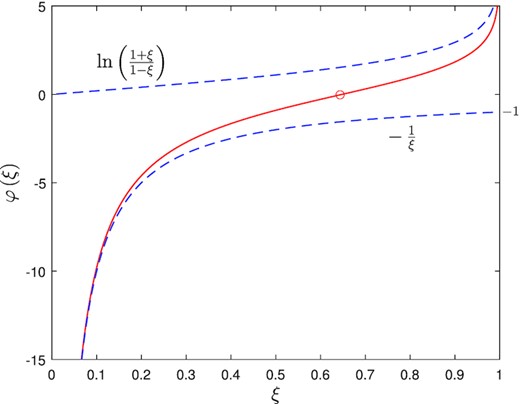
Potential φ(ξ) is plotted versus radius ξ in the ‘proper’ interval 0 < ξ < 1 (solid line). A circle marks the inflection point of the potential at ξ = 0.6436, which is close to the zero ξ₀ = 0.6479, where φ(ξ₀) = 0. The two individual terms of equation (37) are also plotted as dashed lines.

5 SUMMARY AND DISCUSSION

5.1 Summary

This work was motivated by the failure of Newtonian theory and general relativity to explain the flat rotation curves of spiral galaxies, the Tully & Fisher (1977) relation, and the Larson (1981) relations in molecular clouds; and by another flagrant failure to detect any new hypothesized particles that might contribute to the constituents of the so-far fictitious dark matter that was postulated long ago and that unjustly remains a dominant hypothesis in galaxy dynamics for over 40 years despite multiple partial refutations on many fronts (Rott 2017; Bertone & Tait 2018, and Section 1.1). We no longer believe that dark matter exists, and this belief consequently pushes us into the realm of modified theories of gravity related to those proposed first by Milgrom (1983a, b, c, 2015, 2016), and studied extensively also by other researchers (Begeman, Broeils & Sanders 1991; Sanders 1997; McGaugh et al. 2000; Sanders & McGaugh 2002; McGaugh 2012; Famaey & McGaugh 2012, to name a few).

We have investigated several aspects of a new theory of modified dynamics, in which Newton’s G is allowed to vary in space, in a way that reproduces Newtonian gravity in the limit of high surface densities and Milgrom’s MOND in the opposite limit. Our results are encouraging, and they point to a brand-new direction of research on the subject; a direction that will prove to be much less expensive than dark-matter experiments and ‘observations;’ and that will certainly involve considerably fewer free parameters than those employed in Newtonian galaxy models these days. We argue that failure to follow such a new direction would amount to abandoning the scientific method, and this is unacceptable in the physical sciences.

In the bulk of this work, we obtained some fundamental properties stemming from the actions of the gradient dG/dr coupled to the surface density σ(r) = M(r)/r² (Kazanas 1995; Christodoulou & Kazanas 2018, 2019). In particular, we derived the new force law from Poisson’s equation with a modified source and from a Lagrangian formalism (Section 2); the dimensional units of the physical quantities involved (Section 2.3), and their relationships to the obscure integration constants β and γ (Section 3) that appear in the weak-field limit of Weyl gravity (Mannheim & Kazanas 1989; Mannheim 1993; Mannheim & O’Brien 2011, 2012); the Green’s functions in the asymptotic limits of Newtonian gravity and MOND (Appendix  A); the equivalent pressure in the vacuum outside a finite mass distribution (Appendix  B); and the ‘external’ pressure on the surface of a spherical mass of radius r, which also modifies the classical Jeans (1902) criterion for gravitational collapse and fragmentation (Appendix  C). It should be noted that these new pressure terms, as well as the new source function in Poisson’s equation, are not intrinsic properties of space or the vacuum, and they are not hypothetical. Instead, both types of pressure arise from the gradients dG/dr ≠ 0 and dM/dr (inside actual mass distributions, where dM/dr ≠ 0). Furthermore, the surface density σ(r) is featured prominently as a fundamental quantity due to its direct (non-geometric) coupling to dG/dr inside and outside masses.

5.2 Open questions

Four additional results, whose details are not entirely understood or clearly interpreted, and which are worthy of further investigations, are the following:

(a) In Sections 2.3, 3.2, and in Appendix B1, we came across several combinations of physical units characterized by two levels of dichotomy. Table 1 summarizes these levels in a 2 × 2 array representation. The distinction between the two rows is well-understood: constants in row 1 exist only when gravity is present, whereas constants in row 2 are all kinematical in nature, and they exist in spacetime even in the absence of gravity. On the contrary, the distinction between the two columns is much harder to delineate and requires some novel ideas beyond the trite separation of constants based on their perceived (non)cosmological origin. We no longer believe that the presence of c is a link to cosmology because this limiting speed is not imposed on to the material world by ‘the universe;’ it is passively created by the vacuum (which provides the very least, but non-zero resistance to all motions), and it is imposed uniformly on all scales of our universe.

We have investigated the role of the vacuum thoroughly, and we intend to present our results in a companion paper. For our purposes here, it is sufficient to remark that constants in column 2 of Table 1 are independent of the influence of free space, and they are created solely by the physical forces that, just like the vacuum, also affect all scales of the material world, albeit with varying degrees of success. All forces applied on matter create acceleration, and then its combinations with G₀ generate additional units. The order of doing things here apparently matters: first, |${\cal A}_0$| is defined in cell (1,2) of the table, and then, mass M₀ is defined in cell (1,1) by combining vacuum’s c with |${\cal A}_0$|⁠; thus, material objects are created to obey from the outset the limitations set by the vacuum.

(b) In Appendix B1, we derived constants a₀, G₀, and U₀ as the geometric means of various combinations of |${\cal A}_0$| and σ₀. The meaning of this result is under investigation. We tried to find more such known combinations with limited success (see the last two notes in Table 1). It seems, however, that |${\cal A}_0$| and σ₀ are the fundamental constants in this mix of units. So, the surface density effectively comes out of obscurity to become a very important quantity in varying-G gravity (see also Appendix  E) (the Tully-Fisher slope |${\cal A}_0$| is already an established fundamental constant in MOND).

(c) In Section 4, we explored a non-linear coordinate transformation |$x\longmapsto \xi$| that results in a new finite radial coordinate ξ ∈ (0, 1) and clearly separates the two competing terms in the gravitational potential [equation (37)]. The variable scale factor of the contraction is

$$\begin{eqnarray*} \frac{\xi }{x} = g^{-1}=1-\xi ^2\, , \end{eqnarray*}$$

(50)

[see also equations (35) and (45)]. We do not presently have a physical interpretation of why this scaling factor is proportional to 1/G, but we do our best in Appendix  D to work toward a physical description of the role of the varying G in coordinate transformations. One property, however, that we do see clearly in equation (50) is that, to the extent that radius x → ∞ represents an ‘event horizon’ in spherical coordinates, the transformation |$x\longmapsto \xi$| brings this horizon to a finite radial distance of ξ = 1.

(d) In Appendix C3.4, we derived the classical Jeans (1902) criterion for gravitational instability in the Newtonian regime of high surface densities, and a modified, more complex version in the intermediate MOND regime of relatively low surface densities. The latter version includes the range of long-wavelength modes of vibration that get excited at the onset of instability, as well as a critical surface-density value [equations (C32) and (C31), respectively]. A surprising element is that the surface-density threshold of σ_max = 1.25 kg m⁻² ≃ 0.7σ₀ was not derived from the corresponding dispersion relation (C23), but from a mathematical condition that ensures the validity of a truncated series expansion [equation (C16) truncated to order s⁰] in the MOND regime (s → 0⁺). The function f₀(s) involved in this approximation [equation (C6)] is however introduced by self-gravity into the perturbed Poisson equation (C5) in the linearized Jeans stability problem.

5.3 Corrections to Newtonian gravity

Besides the build-in appearance of the fundamental constant |${\cal A}_0 = G_0{}a_0$| and the variation of G that extends into the entire MOND regime, varying-G gravity differs from MOND in that it obeys Gauss’s law exactly (Christodoulou & Kazanas 2019); therefore, there is no ‘external field effect’ (Milgrom 2009; Blanchet & Novak 2011) despite the absence of the strong equivalence principle in varying-G gravity as well (Appendix B1). Hees et al. (2014) used radiometric data of the Cassini spacecraft orbiting Saturn in an effort to measure such an effect. The results were negative (as would be expected in varying-G gravity), although the precise measurements of an anomalous quadrupole moment Q₂ = (3 ± 3) × 10⁻²⁷ s⁻² did manage to reject some of the interpolating functions used in MOND, nearly all of which produce spurious new forces in the regime of intermediate accelerations (Christodoulou & Kazanas 2018).

In varying-G gravity, the correction term to a dominant Newtonian potential, such as that of the Sun in the solar system, is linear (a₀r) and immeasurable at the distance of Saturn from the Sun, despite being much larger than the Q₂ correction term measured by Hees et al. (2014). Although the Cassini data were not fitted with a linear correction term, we can obtain an order of magnitude estimate of the equivalent acceleration coefficient a₂ by recasting the quadrupolar term |$Q_2\, r_{\rm s}^{~2}/3$| in the form |$a_2\, r_{\rm s}$|⁠, where r_s = 9.5826 au is the semimajor axis of Saturn. We find that a₂ ≃ 1.4 × 10⁻¹⁵ m s⁻², a value that is smaller than a₀ by 5 orders of magnitude. So, Saturn is not far enough from the Sun for the correction term a₀r_s to be detected. As is already known (e.g. Blanchet & Novak 2011), corrections due to MOND in the solar system become measurable at the mass-dependent scale of |$(r_M)_\odot = \sqrt{G_0M_\odot /a_0}\simeq 7\times 10^3$| au; and the Cassini deviation Q₂ measured by Hees et al. (2014) (that requires an equivalent distance of ∼8 × 10⁵ au from the Sun for a₂ = a₀) would not be measurable even at the distance of the Oort cloud (∼10⁵ au).

ACKNOWLEDGEMENTS

The authors appreciate the reviewer’ and editors’ considerable efforts to guide them in improving certain aspects of this work. The authors thank the referee, in particular, for providing more citations and raising more questions pertaining to galaxies and galaxy clusters in modified dynamics. In particular, the keen probing of the referee led us to the surprising conclusion described in Section 3.4(b) of Appendix C. NASA support over the years is also gratefully acknowledged. DMC also acknowledges support from NSF-AAG grant No. AST-2109004.

DATA AVAILABILITY

The data used and generated in this study are all included in the manuscript, along with references, where appropriate. More information can be obtained by contacting DMC, the corresponding author (email: [e-mail]).

Footnotes

1

Copernicus credited Aristarchus of Samos in his 1543 treatise De Revolutionibus Orbium Coelestium, but the credit was crossed out prior to publication. This amounts to plagiarism (Spyrou 2004; Greene 2018), and led to a campaign of misinformation that continues to this day—many believe that Copernicus is the father of heliocentric theory. He most definitely is not. Aristarchus of Samos is (Spyrou 2004; Berggren & Sidoli 2007).

2

In contemporary units, |$\sigma _0/(2\pi) = a_0/(2\pi G_0)\simeq 137\, M_\odot \,$|pc⁻² (see, e.g. Donato et al. 2009); but the 2π introduces geometry into the physical constant, and this is not justified. People are generally not aware of this problem; the widespread belief is that only a numerical constant is absorbed into the new definition. We will have much more to say about such units in a companion paper.

3

The series expansions of equation (36) assume interesting forms: as ξ → 0⁺, then |$x \approx \xi + \xi ^3 + \xi ^5 + \xi ^7 + {\cal O}(x^9)$|⁠; and, as ξ → 1⁻, then |$x \approx 1/[2(1-\xi)] - 1/4 - (1-\xi)/8 - (1-\xi)^2/16 - {\cal O}[(1-\xi)^{3}]$|⁠.

4

We dedicate this work to Professor Lynden-Bell, a pioneer in many astrophysical subjects, including of course this one too (Lynden-Bell & Katz 1985). Professor Lynden-Bell’s wisdom and insights will be sorely missed for years to come.

5

In deriving equation (C7), we certainly made use of the ‘Jeans swindle’ in the external-pressure term as well. We dropped the term |$(+1/\rho _0^{~2})(\boldsymbol{\nabla }P_{\rm e0})\rho _1$| along with the term |$(-\boldsymbol{\nabla }\Phi _0)\rho _1$|⁠, because there are no such gradients in the equilibrium state (Section C1).

6

From equation (41), we find that |$g-x= (1+\sqrt{1+4x^2}-2x)/2$|⁠, and the inequality follows from the limits of (g − x) as x → 0 and x → ∞.

7

See also Appendix  C; eliminating the influence of the coordinate system is becoming a unifying theme in this analysis. In a sense, this is understandable since the transformations are not covariant, and the resulting potentials depend on the coordinates used.

APPENDIX A: SECOND-ORDER POISSON’S EQUATION AND GREEN’S FUNCTIONS IN VARYING–G GRAVITY

A1 Poisson’s equation and its source

We consider again the dimensionless form of the gravitational potential φ(x) due to a point-mass M that was given in Section 4, viz.

$$\begin{eqnarray*} \varphi (x) = -\frac{1+\sqrt{1+4x^2}}{2x} +\ln \left(2x + \sqrt{1 + 4x^2}\right)\, , \end{eqnarray*}$$

(A1)

where the dimensionless spherical coordinate x is defined by

$$\begin{eqnarray*} x\equiv r/r_M\, , \end{eqnarray*}$$

(A2)

and the mass-dependent length scale r_M is given by

$$\begin{eqnarray*} r_M = \sqrt{G_0 M/a_0} = \sqrt{M/\sigma _0}\, , \end{eqnarray*}$$

(A3)

where σ₀ = a₀/G₀ is the universal surface-density constant.

We also consider the dimensionless form of Gauss’s law in varying-G gravity (Christodoulou & Kazanas 2019) that leads to Poisson’s equation

$$\begin{eqnarray*} \nabla ^2\varphi (x) = q(x)\, , \end{eqnarray*}$$

(A4)

where the dimensionless source q(x) for a point-mass M at x = 0 is given for radii x ≠ 0 by

$$\begin{eqnarray*} q(x) = \frac{1}{x^2}\frac{d}{dx}g(x)\, , \end{eqnarray*}$$

(A5)

where g(x) = G/G₀ is given by the exact equation (41), viz.

$$\begin{eqnarray*} g(x) = \frac{1}{2}\left(1 + \sqrt{1+4x^2} \right)\, . \end{eqnarray*}$$

(A6)

There are two ways to proceed and they both lead to the same result: we can differentiate twice the potential φ(x) and use equation (A4) to determine the source q(x), or we can differentiate g(x) once and use equation (A5) to obtain q(x). The result has a surprisingly compact form (see also equation (17) in Christodoulou & Kazanas 2019), viz.

$$\begin{eqnarray*} q(x) = \frac{2}{x\sqrt{1+4x^2}}\, , \end{eqnarray*}$$

(A7)

where x ≠ 0. In the Newton–Weyl limit of x → 0⁺, we find that

$$\begin{eqnarray*} q(x)\approx \frac{2}{x} - 4x + 12x^3 - 40x^5 + {\cal O}\left(x^{7}\right)\, . \end{eqnarray*}$$

(A8)

The linear term is identified as a Weyl-like term, although the expansion contains additional higher-order correction terms that do not appear in the Weyl metric. In the deep MOND limit of x → ∞, we find that

$$\begin{eqnarray*} q(x)\approx \frac{1}{x^2} - \frac{1}{8x^4} + \frac{3}{128x^6} -\frac{5}{1024x^8} + {\cal O}\left(x^{-10}\right)\, . \end{eqnarray*}$$

(A9)

It is an interesting property that the leading term switches from ∝ 1/x to 1/x² between these two limiting cases. The power of 2 in the deep MOND limit is a manifestation of the second-order Poisson equation that we used above. In Weyl gravity, the fourth-order Laplacian operator ∇⁴ produces for x ≠ 0 a source of the form

$$\begin{eqnarray*} q_{\rm w}(x) = \frac{8(8x^2-1)}{x(1+4x^2)^{5/2}}\, , \end{eqnarray*}$$

(A10)

whose leading term switches from ∝ − 1/x to ∝ 1/x⁴ between the two limiting cases. The power of 4 in 1/x⁴ shows that the leading term of the q(x) expansion for x → ∞ carries an imprint of the order of the theory.

Equation (A5) is important in another respect: it reveals the physical origin of the source function q(x) in Poisson’s equation. The compact form of q(x) in this equation is entirely due to the variation of g(x) that also couples to the varying surface density σ(x) ∝ 1/x²; so the gradient of g creates a necessary and sufficient condition for σ to contribute to the source. If a constant G₀ were to be assumed instead of G(x) (i.e. if g = 1), then σ(x) would also drop out from the source, in which case the surface density would play absolutely no role, just as it does not in Newtonian gravity. The source q(x) would be zero in the empty space around the point-mass. So, the difference in our case is that the potential in empty space is sourced by the coupling between σ and the gradient of G, and Laplace’s equation does not apply in any vacuum surrounding any amount of matter. This complex issue certainly deserves further investigation and discussion, and we do so in Appendix  B below.

A2 Asymptotic Green’s functions

We return to equation (A1). This potential due to a point-mass located at x = 0 also represents the Green’s function in the exterior space. Its series expansions in the two asymptotic regimes are as follows: In the Newton–Weyl limit of x → 0⁺:

$$\begin{eqnarray*} \varphi (x)\approx -\frac{1}{x} + x - \frac{x^3}{3} + \frac{2x^5}{5} - \frac{5x^7}{7} + {\cal O}\left(x^9 \right)\, ; \end{eqnarray*}$$

(A11)

and in the deep MOND limit of x → ∞:

$$\begin{eqnarray*} \varphi (x)\approx \ln x - \frac{1}{2x} - \frac{1}{16x^2} + \frac{1}{512x^4} - {\cal O}\left(x^{-6}\right)\, , \end{eqnarray*}$$

(A12)

where we dropped an additive constant of (−1 + ln 4).

We see from equation (A11) that the first-order Green’s function at x → 0 contains the familiar Newtonian term −|r − r′|⁻¹ and a repulsive linear term of the form +|r − r′| (as was also found by Mannheim & Kazanas 1994). On the other end, equation (A12) shows that the first-order Green’s function at x → ∞ switches entirely its character to

$$\begin{eqnarray*} \ln \left|r - r^\prime \right|\, , \end{eqnarray*}$$

plus a Newtonian correction of the form |$-\frac{1}{2}\left|r - r^\prime \right|^{-1}$|⁠. We are pleasantly surprised that the above simple modification of G [equation (A6)] that led us into varying-G gravity in the first place (Christodoulou & Kazanas 2018), also encompasses so many different variations of the physics in the two asymptotic regimes.

APPENDIX B: THE REPELLING VACUUM PRESSURE CREATED BY THE VARYING G

Here, we consider the empty space exterior to a spherical mass distribution M(r) of radius r = r_⋆ in varying-G gravity. We examine the effect that the gradient dG/dr produces in pure vacuum, i.e. at distances r > r_⋆. The enclosed mass out to r_⋆, i.e. M(r_⋆), is constant, which makes it possible to use again the mass-dependent length scale |$r_M=\sqrt{M(r_\star)/\sigma _0}$| as defined above for a point-mass and the dimensionless quantities appearing in Appendix  A.

Our goal is to write down an equation for the implied energy density that exists in empty space as a result of the nonzero source term of Poisson’s equation there [|$\sigma \, dG/dr$|⁠; equation (A5)]. This is not vacuum energy stored in the gravitational field, and it is not the conventional cosmological dark energy perhaps stored in a fourth unseen spatial dimension (Trupp 2019). Its origin is the coupling between surface density σ ∝ 1/x² and the gradient dG/dr, as can be clearly seen in equation (A5) above. After years of debates in the literature about the Newtonian asymptotic regime of general relativity (V ≪ c), and the sign of the gravitational field’s internal energy density, we are inclined to believe the physical arguments put forth by Lynden-Bell & Katz (1985)⁴ and, more recently, by Trupp (2019): the Newtonian gravitational field, as well as Einstein’s weak-field gravity, cannot hold energy in the field lines. Instead, Trupp (2019) concluded that externally-sourced dark energy permeating the universe is an indispensable component of both Newtonian gravity and general relativity (but see also Melia 2018, 2019, for an opposing point of view). All this, of course, under the pervasive and highly restrictive assumption of a constant G₀ in space.

B1 A source acting in the vacuum

A varying G creates a source capable of acting in the vacuum. We begin with the source of Poisson’s equation in vacuum [equation (A5)], written out in physical units, viz.

$$\begin{eqnarray*} Q(x) = \left(\frac{a_0}{r_M}\right)\frac{1}{x^2}\frac{d}{dx}g(x)\, , \end{eqnarray*}$$

(B1)

where x = r/r_M and |$r_M=\sqrt{M(r_\star)/\sigma _0}$|⁠. For x > x_⋆, the terms σ ∝ 1/x² and dg/dx are nowhere zero, implying that the vacuum outside the central mass M(x_⋆) is not empty, and Lapace’s equation is not valid in any region of the vacuum. The source Q(x) has dimensions of a₀/r_M, that is, [time]⁻². On the contrary, the vacuum energy density U(x) implied by this term has dimensions of |$[{\rm energy}]{}[{\rm volume}]^{-1}$|⁠, thus

$$\begin{eqnarray*} U(x) = \frac{M(x_\star)}{r_M}Q(x) = \frac{a_0\, M(x_\star)}{r_M^{~~2}}q(x) \equiv U_0\, q(x)\, , \end{eqnarray*}$$

(B2)

where q(x) is given by equation (A7) and the constant U₀ can be simplified to |$U_0 = a_0^{~2}/G_0 = \sigma _0 a_0$|⁠. Notice that U₀ does not depend on c. This is a fundamental property. It implies that the origin of U(x) is not the dimensional vacuum energy density |$M(x_\star)\, c^2/r_M^{~~3} = \sigma _0\, c^2/r_M\propto c^2$|⁠; instead, U(x) originates in the vacuum solely from the varying G(a) function [equation (1)], which has introduced the two constants a₀ and G₀ (see also Table 1). Combinations of these constants behave in a very particular way: |${\cal A}_0$| is the product of a₀ and G₀, and σ₀ is their quotient; therefore, a₀ and G₀ can be realized as the geometric means of the two fundamental constants, |${\cal A}_0$| and σ₀, as follows:

$$\begin{eqnarray*} a_0=\sqrt{{\cal A}_0\, \sigma _0}~~~~ {\rm and} ~~~~G_0=\sqrt{{\cal A}_0\left(\frac{1}{\sigma _0}\right)}\, . \end{eqnarray*}$$

(B3)

These considerations show that σ₀ must be interpreted as a fundamental constant, along with the known fundamental constant |${\cal A}_0$| (Milgrom 2015), and the well-known constants a₀ and G₀ are derived by geometric-mean averaging of the two fundamental constants. Two independent geometric means are formed because of the property of inversion, which is fundamental in forming Lie (1881) groups: in one average, one of the two constants is inverted.

In the same manner, the constant U₀ is found to be the geometric mean of |$\sigma _0^{~3}$| and |${\cal A}_0$|⁠, viz.

$$\begin{eqnarray*} \sqrt{\sigma _0^{~3} {\cal A}_0}= U_0\, ; \end{eqnarray*}$$

(B4)

whereas the geometric mean |$\sqrt{\sigma _0^{~3}(1/{\cal A}_0)}= a_0/G_0^{~2}=\sigma _0/G_0$| (with |${\cal A}_0$| inverted) produces just a composite constant, viz.

$$\begin{eqnarray*} \sqrt{\sigma _0^{~3}\left(\frac{1}{{\cal A}_0} \right)}=\frac{U_0^{~2}}{a_0^{~3}}\, , \end{eqnarray*}$$

(B5)

of a lesser interest. Based on the groups of units collected in Table 1, this appears to be an important property: only low powers of the two fundamental constants produce new unblended characteristic constants [as in equations (B3) and (B4)]; whereas progressively higher powers result mostly in composite units [as in equation (B5)]. Such composite units do however deserve to be investigated about possible calibrations they could provide for the sources of gravity (see Appendix  E below, for a case study involving various surface densities).

B2 Vacuum energy density and pressure

Energy density U has dimensions of pressure P. Thus, we define a dimensionless vacuum pressure p_v ≡ U/U₀, and we find from equations (B2) and (A7) that

$$\begin{eqnarray*} p_{\rm v}(x) = \frac{2}{x\sqrt{1 + 4x^2}} \gt 0\, . \end{eqnarray*}$$

(B6)

It is easy to show that dp_v/dx < 0, thus the p_v-gradient is pushing out into the vacuum and away from the central mass. Its characteristic magnitude is found to be |$U_0 = a_0^{~2}/G_0\simeq 1.35$| GeV m⁻³ or 2.16 × 10⁻¹⁰ Pa. The corresponding volume density in the vacuum is found to be ρ₀ = U₀/c² = 2.40 × 10⁻²⁷ kg m⁻³, i.e. six orders of magnitude lower than the typical density of the interstellar medium.

These values may be interpreted as a cosmological-constant problem being present in varying-G gravity as well. We think that would be the wrong conclusion. There is no such problem in our case because this energy density does not belong to the vacuum, it just lives there. Interpreted as outward-pushing pressure, this new type of ‘dark energy’ belongs exclusively to gravity, to the positive gradient dG/dr to be more precise, and this gradient is not a quantum oscillator. The present vacuum itself does not oscillate either, because it possesses no (material or energetic) property that could possibly fluctuate in the context of this or any other physical theory; in fact, the vacuum here does not possess any other property besides ‘emptiness.’ The density and pressure of the vacuum described above are just convenient analogues that describe the cosmological influence of σ(dG/dr) in empty space, but they do not ascribe or imprint any physical properties to the vacuum. For this reason, the uncertainty principle is also not relevant to the present state of absolute emptiness of free space, and this is why the calculations presented here do not miss by 120 orders of magnitude when compared to observations (see, e.g. the determination of U₀ above).

B3 Non-cosmological Scales

The asymptotic expansions of equation (B6) are those of q(x) shown in equations (A8) and (A9) above. As x → ∞, then p_v → 0 as 1/x² (same as for σ(x) because dg/dx → 1). As x → 0, then p_v → ∞ as 2/x and

$$\begin{eqnarray*} P_{\rm v}(x)\approx 2U_0/x{}, \end{eqnarray*}$$

at small (non-cosmological) scales. For example, on the surface of the sun, where x_⊙ = r_⊙/r_M = 6.6 × 10⁻⁷ ≪ 1 and σ_⊙ = 4 × 10¹² kg m⁻², the vacuum pressure is |$P_{\rm v}(x_\odot) = 2\sigma _0\sqrt{{\cal A}_0\sigma _\odot }\approx 4$| PeV m⁻³ (P = 10¹⁵) or 6.5 × 10⁻⁴ Pa, thus negligible. On the horizon of an 8M_⊙ black hole or on the surface of a canonical neutron star (r_⋆ = 10 km, M(r_⋆) = 1.4M_⊙), the vacuum pressure rises by five orders of magnitude to 0.34 ZeV m⁻³ (Z = 10²¹) or 54 Pa, yet it remains negligible. The value of P_v on the surface of the Earth is lower than the solar value. On the contrary, P_v-values on the horizons of supermassive black holes are lower than the compact stellar value of 0.34 ZeV m⁻³ determined above.

This non-monotonic behaviour versus mass is certainly not due to the normalizing constant |$U_0=a_0^{~2}/G_0$|⁠, so we turn to the variations of |$P_{\rm v}(x)\propto 1/x = r_M/r\propto \sqrt{\sigma }$| for x ≪ 1. For collapsed objects with a Schwarzschild radius R_S, then |$P_{\rm v}(R_{\rm S})\propto 1/\sqrt{R_{\rm S}}$|⁠, and the smallest, least massive black hole will be the one with the highest vacuum pressure on its horizon. That could be a 1.4M_⊙ neutron star that has collapsed to a black hole with R_S ≃ 4 km, in which case P_{v, max} ≃ 0.8 ZeV m⁻³ or 130 Pa. The extreme case of a 1M_⊙ black hole with R_S ≃ 3 km and σ ≃ 2 × 10²³ kg m⁻² is only slightly different, yet an instructive upper limit:

$$\begin{eqnarray*} (P_{\rm v})_{\rm max} \simeq 1~{\rm ZeV\, m}^{-3} \simeq 150~{\rm Pa}\, , \end{eqnarray*}$$

(B7)

where, again, Z = 10²¹ in the SI system of units.

B4 The Planck scale

Only at the Planck scale, where the universe could also have experienced quantum effects, do we find a much higher value of the vacuum pressure. We use the modern Planck mass M_P = 2.176 × 10⁻⁸ kg and its Schwarzschild radius |$R_{\rm SP} = 2\, L_{\rm P}$|⁠, where L_P = 1.616 × 10⁻³⁵ m is the modern Planck length (2018 CODATA values; Tiesinga et al. 2021). We find a surface density of |$\sigma _{\rm P} = M_{\rm P}/R_{\rm SP}^{~~\, 2} = 2\times 10^{61}$| kg m⁻² and a vacuum pressure of

$$\begin{eqnarray*} (P_{\rm v})_{\rm P} \simeq 10^{40}~{\rm eV\, m}^{-3} \simeq 1.5~{\rm ZPa}\, , \end{eqnarray*}$$

(B8)

at the Planck scale. This pressure is 19 orders of magnitude larger than the ideal maximum stellar compact value shown in equation (B7).

APPENDIX C: GRAVITATIONAL INSTABILITY IN VARYING-G GRAVITY

C1 A swindle?

The Jeans swindle (Jeans 1902; Binney & Tremaine 2008) is a bizarre mathematical tool, so bizarre that it has to be good. Indeed, we presently know this tool works well because of the remarkable result it has achieved (the famous Jeans instability criterion for gravitational collapse and fragmentation). The methodology was invented by Jeans in a study of a highly idealized and totally unrealistic medium with the following properties: the medium is isolated, infinite in extent, homogeneous, isotropic, compressible (isothermal or adiabatic), self-gravitating, and in hydrostatic equilibrium. Jeans intended to study the struggle between self-gravity and thermal pressure in the small perturbations that would arise randomly within the medium, and to determine the linear stability of the system. The so-called swindle occurred when Jeans eliminated all zeroth-order equilibrium gradients from the linearized perturbation equations. We now know that was the right thing to do, although Jeans did not provide any justification. Other researchers eventually picked up on this omission, they judged that Jeans did not pay attention to the underlying assumptions, and they declared that the unjustified calculation was wrong, and it just happened to give the right answer. Such appeals to chance are not in line with the scientific method. Unwillingness to search for reasons, causes, and justifications of a calculation that produced a solid result is not part of the methodologies adopted in the physical sciences.

We do not think there is a swindle in the above story. In an idealized system such as the above medium, there is no center or preferred direction to attach a coordinate system. But we must do so anyway, in order to study the evolution of perturbations in the medium. Therefore, we must proceed with considerable caution. The adopted coordinate system artificially introduces symmetries that do not exist in the actual medium (e.g. spherical symmetry), and we must find them and eliminate them before they lead us astray. Specifically, we must not let equilibrium gradients operate along the principal axes (they do not operate within the uncoordinated medium in any direction), and this takes care of directional derivatives as well. Not doing so would lead us to a different equilibrium state than that envisioned for the original idealized medium.

This is actually what takes place when we study a similar but finite medium. The gradients that we use in equilibrium are subject to the symmetries that we impose, and they still cannot determine a unique solution, unless we also impose additional boundary conditions. The externally imposed boundary conditions make the gradients ‘do the right thing.’ So, this is what may have occurred in the calculation of Jeans; knowing that the gradients are unable to do the right thing (that is, disappear after the introduction of the frame), and since he could not impose boundary conditions on the infinite medium, he eliminated the equilibrium gradients everywhere in the domain. In retrospect, this turns out to be an ingenious way of imposing physical conditions on a system for which the Cauchy problem is either ill-defined or cannot be repaired; and altogether a brand-new method of tackling such idealized systems with no boundaries that cannot be specified fully in the Cauchy sense.

Therefore, to impose the original uncoordinated equilibrium properties on to the linearized equations, we must eliminate all equilibrium gradients upon introduction of a coordinate frame. Furthermore, since the gradients are all zero in equilibrium, Gauss’s law and Poisson’s equation become invalid. Gauss’s law, for instance, relies on a simply-connected surface integral around a center (point or plane), whereas no such center exists in the original medium before the introduction of the coordinate frame; and Poisson’s equation is derived from Gauss’s law.

When we introduce small perturbations to the infinite medium, the situation changes. The perturbations are precisely designed according to the symmetries of the chosen frame. For example, we introduce a spherical coordinate system centered at some arbitrary point in Section C3 below because we intend to study the time evolution of spherical modes of vibration. Then, the gradients of the perturbed quantities acquire solid physical meaning, and Gauss’s law is valid for the imposed perturbations—they both use the same symmetry that was established by the introduction of the appropriate coordinate frame.

C2 Recent history

Adhering to the scientific method, Kiessling (2003) and Falco et al. (2013) attempted to explain why the swindle works so well in a static universe with a cosmological constant, and in an expanding universe such as our universe, respectively. However, such efforts have nothing to say about possible (in)consistencies in the original analysis of Jeans (1902). In fact, these authors begin by adopting the premise that there is a swindle in the original calculation, and they attempt to justify it after the fact. In this sense, both approaches are conceptually different from our approach laid out in Section C1 above.

Kiessling (2003), however, in his introduction takes the same position as we did about the invalidity of Poisson’s equation in the equilibrium state, and he actually proves that Poisson’s equation returns to validity in the analysis of small perturbations. A potential issue that we must think about concerning Kiessling’s derivation is that reducing the cosmological equations to the pure Newtonian case by taking the limit of vanishing cosmological constant could violate energy conservation in a finite system. In particular, this reduction could, under ordinary circumstances, lead to the appearance of structural instability in the solutions (Thom 1976; Drazin & Reid 1981; Christodoulou, Contopoulos & Kazanas 1996).

In the next subsection, we carry out the original calculation of Jeans in the context of varying-G gravity that introduces additional terms into the linearized equations. We intend to ‘swindle’ our readers ‘more than Jeans (1902) did,’ by discarding an additional pressure-gradient equilibrium term that owed its fleeting existence to the symmetry imposed by the attached spherical coordinate frame.

C3 Linear stability analysis in varying-G gravity

In the past, we have made an attempt to study varying-G gravity in an infinite homogeneous medium (Christodoulou & Kazanas 2019), but we did not apply linear perturbation theory to the standard hydrodynamical equations. We return to this problem here, with an eye on gravitational instability and the famous Jeans (1902) stability criterion.

C3.1 Source function and external pressure

We rely on the source function obtained previously for a homogeneous and isotropic medium. We attach a spherical coordinate system centered at an arbitrary point within the medium. Because the equilibrium density ρ₀ is constant and the mass M(r) enclosed within any arbitrary radius r is not constant, we are not permitted to use mass-dependent scales (r_M and M). The characteristic length scale L of the medium now is

$$\begin{eqnarray*} L = \frac{3a_0}{4\pi G_0\rho _0} = \frac{3}{4\pi }\frac{\sigma _0}{\rho _0} \, ; \end{eqnarray*}$$

(C1)

the normalized radius r/L represents dimensionless surface density s = σ/σ₀ (i.e. s = r/L for any enclosed mass of M(r) = 4πρ₀r³/3); and the source is expressed conveniently as a function of s (Christodoulou & Kazanas 2019), viz.

$$\begin{eqnarray*} Q(s) = 2\pi G_0\rho _0{} q(s) \, , \end{eqnarray*}$$

(C2)

where

$$\begin{eqnarray*} q(s) = 1 + \frac{s+10/3}{\sqrt{s^2 + 4s}} \, . \end{eqnarray*}$$

(C3)

Thus, on any chosen spherical surface of radius r, we can define the dimensional energy density U(s) = [M(L)/L]Q(s) or external pressure P_e(s) by

$$\begin{eqnarray*} U(s) = P_{\rm e}(s) = \frac{3}{2}\frac{a_0^{~2}}{G_0}q(s) \, . \end{eqnarray*}$$

(C4)

It is easy to show that dP_e/ds < 0, thus this pressure gradient is pushing outward and away from the spherical surface of radius r = Ls ∝ s. Its characteristic magnitude is found to be larger than the vacuum pressure (Section B2) by a factor of 3/2, i.e. |$3a_0^{~2}/(2G_0)\simeq 2.0$| GeV m⁻³.

C3.2 Linearized equations

Function q(s) [equation (C3)] affects and effectively modifies the properties of the linearized perturbations in an infinite isothermal medium (the ‘Jeans-Newton’ equations (36)-(38) in Kiessling 2003). Perturbations of the source (C2) are introduced in the linearized Poisson equation that now reads

$$\begin{eqnarray*} \nabla ^2\Phi _1 = 2\pi G_0 f_0(s)\rho _1 \, , \end{eqnarray*}$$

(C5)

where subscript 1 identifies perturbed quantities, and

$$\begin{eqnarray*} f_0(s) = 1 + \frac{s\left(s^2 + 6s + 20/3 \right)}{(s^2 + 4s)^{3/2}} \gt 0 \, . \end{eqnarray*}$$

(C6)

Perturbations of the external pressure (C4) are introduced in the linearized equation of motion that now reads⁵

$$\begin{eqnarray*} \frac{\partial \boldsymbol{{\bf v_1}}}{\partial t} = -\frac{1}{\rho _0}\left[c_{\rm st}^{~2} - 2 h_0(s) c_{\rm e}^{~2}\right]\, \boldsymbol{\nabla }\rho _1 \, -\, \boldsymbol{\nabla }\Phi _1\, , \end{eqnarray*}$$

(C7)

where

$$\begin{eqnarray*} c_{\rm st}^{~2} = c_{\rm s}^{~2} + c_{\rm t}^{~2}/3\, , \end{eqnarray*}$$

(C8)

is the effective kinetic support in the medium that typically goes against gravity (and, here, against external pressure as well), given by the sum of the isothermal sound speed squared (⁠|$c_{\rm s}^{~2}$|⁠) and the one-dimensional velocity variance (⁠|$c_{\rm t}^{~2}/3$|⁠) of the turbulent motions (as derived first by Chandrasekhar 1951);

$$\begin{eqnarray*} c_{\rm e}^2\equiv a_0^{~2}/(G_0 \rho _0) = \sigma _0 a_0/\rho _0\, ; \end{eqnarray*}$$

(C9)

and

$$\begin{eqnarray*} h_0(s) = \frac{s(s + 5)}{(s^2 + 4s)^{3/2}} \gt 0 \, . \end{eqnarray*}$$

(C10)

Support due to turbulence (⁠|$c_{\rm t}^{~2}/3$|⁠) must be included in the calculation because, in many astrophysical settings, c_t ≫ c_s. On the contrary, the linearized continuity equation

$$\begin{eqnarray*} \frac{\partial \rho _1}{\partial t} + \rho _0\boldsymbol{\nabla \cdot {\bf v_1}} = 0\, , \end{eqnarray*}$$

(C11)

remains the same.

If there is a striking feature in these modified linearized equations, this must be the behavior of the external-pressure term |$+2h_0c_{\rm e}^{~2}(\boldsymbol{\nabla }\rho _1)/\rho _0\,$| in the equation of motion (C7). Although in equilibrium the external pressure [equation (C4)] would be repulsive, if it could operate (and it will be repulsive in more realistic finite media); in the perturbed state, the external-pressure disturbance pushes inward and cooperates with self-gravity; thus this perturbation acts as a binding pressure at every radius r inside the medium.

C3.3 Dispersion relation and stability

We find then, that external pressure, just like self-gravity, acts to suppress the kinetic support due to thermal and turbulent motions in the dispersion relation of spherical wave-like disturbances springing up in the infinite medium. The dispersion relation of superposed waves is found easily by solving the above system of equations (e.g. Kiessling 2003; Binney & Tremaine 2008). We find that the frequencies ω of the waves are given by the relation

$$\begin{eqnarray*} \omega ^2 = \left(c_{\rm st}^{~2} - 2{} h_0{} c_{\rm e}^{~2}\right) k^2 \, -\, \frac{1}{2}f_0{} \Omega _{\rm J}^{~2} \, , \end{eqnarray*}$$

(C12)

where k is the wavenumber that corresponds to a wavelength of λ = 2π/k, and

$$\begin{eqnarray*} \Omega _{\rm J}^{~2} = 4{}\pi {} G_0{}\rho _0 \, , \end{eqnarray*}$$

(C13)

is the familiar gravitational (Jeans) frequency. So, it is two against two, and three out of four terms have been cast as pressure-like terms. The medium is linearly stable to low-amplitude disturbances when ω ² > 0 and the internal kinetic terms overpower the combined attractive forces of self-gravity and external pressure. Marginal stability is signaled by ω = 0 when the medium is on the verge of instability. In this case, as well as for ω ² < 0, it is only a matter of time before some long-wavelength modes of vibration get excited and nonlinear instability sets in (Chandrasekhar 1951).

Equation (C12) appears to be a significant departure from the conventional Jeans (1902) stability criterion, but this is not so in the Newtonian asymptotic regime. In the Newtonian framework (G = G₀ = constant), where the original Jeans criterion was derived, the external pressure disappears (h₀ = 0) and f₀ = 2, restoring thus the familiar Jeans dispersion relation.

C3.4 Jeans instability in the two asymptotic limits

The series expansions of functions f₀(s) and h₀(s) [equations (C6) and (C10), respectively] in the two asymptotic regimes of varying-G gravity are as follows: In the Newton–Weyl limit of s → ∞:

$$\begin{eqnarray*} f_0(s)\approx 2 + \frac{2}{3s^2} - \frac{10}{s^4} + {\cal O}\left(1/s^5\right)\, , \end{eqnarray*}$$

(C14)

and

$$\begin{eqnarray*} h_0(s)\approx \frac{1}{s} - \frac{1}{s^2} + \frac{10}{s^4} - {\cal O}\left(1/s^5\right)\, . \end{eqnarray*}$$

(C15)

In the deep MOND limit of s → 0⁺:

$$\begin{eqnarray*} f_0(s)\approx \frac{5}{6\sqrt{s}} + 1 + \frac{7\sqrt{s}}{16} - {\cal O}\left(s^{3/2}\right)\, , \end{eqnarray*}$$

(C16)

and

$$\begin{eqnarray*} h_0(s)\approx \frac{5}{8\sqrt{s}} - \frac{7\sqrt{s}}{64} + {\cal O}\left(s^{3/2}\right)\, . \end{eqnarray*}$$

(C17)

Considering the leading terms of the series expansions, we examine the onset of instability in the two usual asymptotic regimes:

(a) Newtonian Regime.—For s → ∞, equation (C12) takes the form

$$\begin{eqnarray*} \omega ^2 = \left(c_{\rm st}^{~2} - \frac{2}{s}c_{\rm e}^{~2}\right) k^2 \, -\, \Omega _{\rm J}^{~2} \, , \end{eqnarray*}$$

(C18)

and since the external-pressure term is negligible, the Jeans (1902) dispersion relation is essentially recovered. The critical wavenumber for marginal stability in the s → ∞ case is the so-called Jeans wavenumber

$$\begin{eqnarray*} k_{\rm J}=\frac{\Omega _{\rm J}}{c_{\rm st}} \, , \end{eqnarray*}$$

(C19)

and all modes of vibration with k < k_J (wavelengths λ > λ_J) are bound to be unstable.

A small but nonzero |$(2/s)c_{\rm e}^2$| term in equation (C18) inserts a minor correction to the critical wavenumber. To order 1/s, we find that, for instability

$$\begin{eqnarray*} \kappa \, \ge \, 1 - \frac{2\eta }{s} \, , \end{eqnarray*}$$

(C20)

where, for convenience, we used the following definitions of dimensionless quantities:

$$\begin{eqnarray*} \eta \equiv (c_{\rm e}/c_{\rm st})^2 \, , \end{eqnarray*}$$

(C21)

and

$$\begin{eqnarray*} \kappa \equiv (k_{\rm J}/k)^2 \, . \end{eqnarray*}$$

(C22)

Equation (C20) shows that, to order 1/s, the marginal value of k is slightly larger than the well-known Jeans threshold of k_J by a factor of η/s ≪ 1. For slightly larger values of the ratio η/s, some more disturbances become unstable; and pushing the approximation to its limit η/s = 1/2, then κ ≥ 0, and all normal modes go unstable, down to the virtual zero-wavelength mode.

(b) MOND Regime.—For s → 0⁺, equation (C12) takes the form

$$\begin{eqnarray*} \omega ^2 = \left(c_{\rm st}^{~2} - \frac{5}{4\sqrt{s}} \, c_{\rm e}^{~2}\right) k^2 \, -\, \frac{1}{2}\left(\frac{5}{6\sqrt{s}} + 1\right) \, \Omega _{\rm J}^{~2} \, , \end{eqnarray*}$$

(C23)

to approximation order s⁰ [equations (C16) and (C17)]. From the second parenthesis on the right, we obtain a necessary and sufficient condition for the truncated series expansion (C16) to be accurate, viz. |$1 \ll 5/(6\sqrt{s\, })$| or, equivalently,

$$\begin{eqnarray*} s\ll (5/6)^2\approx 0.6944\, . \end{eqnarray*}$$

(C24)

From the first parenthesis on the right, we obtain a necessary condition for stability, namely s > (5η/4)², and pushing the approximation (C24) to its limit, the two conditions combined result in an interval of s-values for modes of interest, [s_min, s_max], viz.

$$\begin{eqnarray*} s_{\rm min}=\frac{25}{16}\eta ^2 \, \lt \, s \, \le \, \frac{25}{36}=s_{\rm max} \, . \end{eqnarray*}$$

(C25)

For s ≤ s_min, all modes are unstable because ω² < 0 in the dispersion relation (C23). In practice, however, we do not expect the surface densities to fall below the s_min threshold, so we focus on the upper limit s_max.

To order s⁰, the criterion for instability ω² ≤ 0 becomes

$$\begin{eqnarray*} \kappa \, \ge \, \frac{4\sqrt{s}-5\eta }{~2\sqrt{s}+5/3} \, . \end{eqnarray*}$$

(C26)

For s = s_max, then κ ≥ 1 − 3η/2, and, once again, the marginal value of k is slightly larger than the Jeans threshold of k_J by a factor of 3η/4 ≪ 1/2.

To obtain a practical form of the instability criterion (C26), we rewrite equation (C22) in terms of the wavelength of a mode λ = 2π/k and a natural length scale λ₀ that arises in a homogeneous medium, such that

$$\begin{eqnarray*} \ell = \lambda /\lambda _0\, , \end{eqnarray*}$$

(C27)

viz.

$$\begin{eqnarray*} \kappa = \eta {}\ell ^2 \, , \end{eqnarray*}$$

(C28)

where

$$\begin{eqnarray*} \begin{array}{lllll}\lambda _0 &\equiv & \sqrt{\pi \, } (4\pi /3) L &=& 7.4244{}L\\ &=& \sqrt{\pi \, }(\sigma _0/\rho _0) &=& 1.7725{}(\sigma _0/\rho _0)\\ \end{array} . \end{eqnarray*}$$

(C29)

Substituting s = s_max from equation (C25) and κ from equation (C28) into equation (C26), the criterion for the longer-wavelength modes going unstable becomes

$$\begin{eqnarray*} \lambda \, \ge \, \frac{\lambda _0}{\sqrt{\eta \, }} \, , \end{eqnarray*}$$

(C30)

where η ≪ 2/3 is given by equation (C21), and the implicit condition that s = s_max determines the characteristic surface density for the onset of instability at the longer wavelengths, viz.

$$\begin{eqnarray*} \sigma _{\rm max} = (5/6)^2\sigma _0 = 1.25~{\rm kg~m}^{-2}\, . \end{eqnarray*}$$

(C31)

This threshold is applicable to all systems, finite or infinite. In a finite system, however, the longest unstable wavelength will be of the order of its characteristic size (diameter) d; thus, we can specify the shortest interval of λ-values at the onset of dynamical instability, that occurs at the highest permitted surface density σ_max (equation (C31)), as follows:

$$\begin{eqnarray*} \lambda _0/\sqrt{\eta } ~\le ~ \lambda ~\le ~ d \, . \end{eqnarray*}$$

(C32)

The instability strip specified by this equation, in conjunction with the critical surface density (C31), constitutes the main result of our gravitational instability analysis in the MOND regime (and also in the regime of intermediate accelerations a ≳ a₀; see below). Finally, in the idealized case, in which we also push the approximation of η to its limit (η → 2/3 from below), we find that s_min = s_max = (5/6)², and that virtually all normal modes become unstable at this surface density [i.e. 0 ≤ λ ≤ d in place of equation (C32)].

We conclude this analysis with a rather surprising realization: The critical wavelength |$\lambda _0/\sqrt{\eta }$| [equations (C30) and (C32)] in our approximation is none other than the classical Jeans wavelength! Substituting equations (C29), (C21), (C1), and (C9) into equation (C30) and squaring both sides, we find that

$$\begin{eqnarray*} \lambda ^2 \ge \lambda _J^{~2} = \frac{\pi \, c_{\rm st}^{~2}}{G_0\rho _0}\, , \end{eqnarray*}$$

(C33)

which is effectively equation (5.46) in Binney & Tremaine (2008) for the classical Jeans wavelength λ_J. This result explains the uncompromising robustness of the classical Jeans (1902) criterion over the past 120 years. It becomes now obvious that our linear stability analysis in the MOND regime only manages to supplement this incredibly robust instability criterion with just an additional critical surface density [equations (C24) and (C31)].

APPENDIX D: THE SCALE FACTOR |${\it g}^{{\bf \, -1}}$| VIEWED AS A RADIAL COORDINATE

We would like to investigate how g(x) [equation (A6)] operates on the radial coordinate x in the two separated terms of the potential (37). We return, once again, to the fundamental equation (A1), and we recast it in the equivalent form

$$\begin{eqnarray*} \varphi (x, g)=-\frac{g}{x} \, +\, \ln \left(\frac{g+x}{g-x}\right) , \end{eqnarray*}$$

(D1)

where g ≥ 1 and⁶ 1/2 < g − x < 1 for all x > 0. The Newtonian term −g/x is structured precisely as already known, but the logarithmic MOND term holds a surprise. The obvious way to interpret its argument is that g plays now the role of the coordinate, and ±x represents a shift of g to the left/right.

It would be unorthodox (and against general covariance) if we kept the ±x shift in equation (D1) because this shift is variable. So, the evidence leads us to eliminate⁷ x and consider g as the only ‘coordinate’ left in the potential. Thus, we return to equation (A6), and we solve it for x, viz.

$$\begin{eqnarray*} x = \sqrt{(g-1)g{}}\, , \end{eqnarray*}$$

(D2)

and this holds another surprise: x is the geometric mean of g and its measure (g − 1) away from its minimum g_min = 1. Then, as in Appendix B1, we also calculate the inverted geometric mean of (g − 1) and 1/g, and we find that

$$\begin{eqnarray*} \sqrt{(g-1)\left(\frac{1}{g}\right)} \, =\, \xi \, . \end{eqnarray*}$$

(D3)

Thus, the scope of geometric averaging that we described for physical constants in Appendix B1 extends to the radial coordinates x and ξ; and the new coordinate turns out to be |$\xi = \sqrt{1 - g^{-1}{}}$|⁠, a simple function of the scale factor g⁻¹ that gives the potential in the transformed form of equation (37), or equivalently, in the rather complicated form

$$\begin{eqnarray*} \varphi \left(g^{-1}\right)=\frac{-1}{\sqrt{1 - g^{-1}{}}} \, +\, \ln \left(\frac{1+\sqrt{1 - g^{-1}{}}}{1-\sqrt{1 - g^{-1}{}}}\right) , \end{eqnarray*}$$

(D4)

which shows the potential φ as a function of the scale factor g⁻¹ only.

Now, we can examine how the scale factor g⁻¹ (all by itself) regulates the potential in the two asymptotic regimes: In the Newtonian regime, where g⁻¹ → 1⁻, the dominant term in the potential is

$$\begin{eqnarray*} \frac{-1}{\sqrt{1-g^{-1}}} \, ; \end{eqnarray*}$$

whereas in the MOND regime, where g⁻¹ → 0⁺, the dominant term in the potential assumes the form

$$\begin{eqnarray*} -\ln \left(g^{-1}\right)\, . \end{eqnarray*}$$

The difference between the two limiting cases is now evident: the measure of the ‘distance’ of g⁻¹ from its maximum value of (g⁻¹)_max = 1 determines the Newtonian term, whereas the scale factor g⁻¹, all by itself, determines the strength of the MOND term. In the former case, the distance

$$\begin{eqnarray*} 1-g^{-1} = \frac{G - G_0}{G}\, , \end{eqnarray*}$$

(D5)

effectively measures the relative deviation of the Newtonian value G₀ from the actual value of G (where G ≳ G₀). In the latter case, the predominance of the magnitude of g⁻¹ suggests an unambiguous universal (albeit non-cosmological) origin for MOND (Milgrom 1983a), the empirical theory that ushered us all to the era of modified dynamics.

In Table D1, we list the critical values of variables derived from the inflection point of φ(ξ) [equation (37) and Fig. 1], the only critical point displayed by the potential φ(ξ). These values are thought to represent the separatrix between the two asymptotic regimes. The following significant properties are seen in the data of Table D1:

• The extent of the Newtonian regime (Δξ ≈ 0.64) in ξ-space is longer than that of the MOND regime.

• Since x ≈ 1, then the critical spherical radius is r ≈ r_M (where |$r_M=\sqrt{M/\sigma _0}$|⁠), so the mass-dependent radius r_M also indicates the region of dominant Newtonian dynamics.

• Since 1 − g⁻¹ ≈ 0.4, the Newtonian regime appears to shrink substantially in g⁻¹-space.

• The separatrix |$\sigma \, ({\rm SI}) = 1.5$| falls between the universal unit σ₀ = 1.8 kg m⁻² and the critical value σ_max = 1.25 kg m⁻² in the Jeans infinite, homogeneous, and isotropic model (equation (C31)). So, Jeans instability sets in near the separatrix |$\sigma \, ({\rm SI})$|⁠, in the regime of intermediate accelerations; and this is why it proved so difficult to derive its connection to surface density.

• The critical values of a and |${\cal A}$| are larger than the MOND constants a₀ and |${\cal A}_0$|⁠, respectively. Thus, these values also belong to the regime of intermediate accelerations.

Table D1.

Critical values separating the two asymptotic regimes (inflection point of the potential φ(ξ) in Fig. 1).

Variable	Definition	Critical value
ξ	φ″(ξ) = 0	0.6436
x	ξ/(1 − ξ2)	1.0987
s	1/x2	0.8285
g	1/(1 − ξ2)	1.7071
g−1	1 − ξ2	0.5858
1 − g−1	ξ2	0.4142
σ (SI)	σ0s	1.5
G (SI)	G0g	|$1.14\times 10^{-10} \, \simeq \, 1.7{}G_0$|
a (SI)	Gσ	|$1.70\times 10^{-10} \, \simeq \, 1.4{}a_0$|
|${\cal A}$| (SI)	Ga	|$1.93\times 10^{-20} \, \simeq \, 2.4{}{\cal A}_0$|

APPENDIX E: FIVE SURFACE DENSITIES AND A BRAND-NEW ORIGIN OF GRAVITY

We recognized from the outset that gravity is produced by the interaction between two fundamental agents, G(r) and M(r), but we treated them differently because we thought that they are different. We were wrong on both counts. A mere look at the source term on the right-hand side of equation (2) reveals our preconceived notions. We identified the coefficient of dG/dr to be σ(r) = M(r)/r², but we missed the coefficient of dM/dr, which corresponds to just another surface density, that of σ_g(r) = G(r)/r². From this seemingly innocuous observation, it becomes clear that M and G are not the sources of gravity—their surface densities are. Thus, we must rectify our approach, and the payoff is a substantial boost in clarity.

We pursued the above analogy of surface densities further, and we found five different surface densities (SDs) of interest to varying-G gravity. These SDs are listed in Table E1. The first three SDs are fundamental, whereas the last two can be constructed from combinations of the first three SDs. SDs (4) and (5) are only listed to highlight the high degrees of inversion symmetries that the SDs and their units exhibit. Furthermore, SD (4) set us on the present path, when we were surprised to find it corresponding to the composite constant |$U_0^{~2}/a_0^{~3}$| (Appendix B1), rather than a fundamental unit of the theory.

Table E1.

SDs in varying-G gravity.

No.	SD	Definition	Unit
(1)	of (GM)(r)	σgm = GM/r2 = a(r)	a0
(2)	of M(r)	σm = M/r2 = σ(r)	a0/G0 = σ0
(3)	of G(r)	σg = G/r2	a0/Mc (*)
		σg × σm = GM/r4	U0/Mc (*)
(4)	of (M/G)(r)	σmog = (M/G)/r2	|$U_0^{\, 2}/a_0^{\, {}3}$|
(5)	of (G/M)(r)	σgom = (G/M)/r2	|$a_0/M_{\rm c}^{\, 2}$| (*)

Note.(*) For some constant mass M_c and some constant length scale L_c, such that |$M_{\rm c}/L_{\rm c}^{\, {}2}=\sigma _0$|⁠. Given M_c, this relation determines the length scale L_c where σ(r) = σ₀. For example, L_c = 12.2 au for the earth, and L_c = 7 × 10³ au for the sun (see also Section 5.3).

Revealing as it may be, the list of SDs in Table E1 holds quite a few surprises:

• SD (1) shows that the gravitational field a(r) is exactly equal to the SD σ_gm, whereas the row below SD (3) shows the specific energy density of the field σ_g × σ_m. These two rows eloquently summarize the dynamics of varying-G gravity. Newtonian dynamics has no such properties: its acceleration is G₀σ_m, and its specific energy density is (G₀/r²)σ_m, where now the 1/r² can only be interpreted as a geometric curvature term. The difference is quite striking: σ_g × σ_m is a purely dynamical density, and geometry is completely absent; in contrast, geometry has crept into the Newtonian density, which is the hidden impetus for the need to develop general relativity or Weyl gravity. In hindsight, one could have arrived at the same conclusions by focusing on the variation of G(r) in equation (6) or (10) and the implications of keeping Newton’s G constant.

• Thus, SD (1) takes us back to reconsider the integral in the potential (7). Undoing the simplifications, we write the gravitational potential formally in spherical radial coordinates as

  $$\begin{eqnarray*} \Phi (r) = \frac{1}{4\pi }\int {\left[\sigma _{\rm g}(r)\times \sigma _{\rm m}(r)\right]\, d{\cal V}}\, , \end{eqnarray*}$$

  (E1)

  where |$d{\cal V}=4\pi r^2 dr$| is the volume element. The source of gravity is in plain sight in this equation. This structure also implies that, contrary to our past experiences, G and M are certainly not fundamental quantities in varying-G gravity. They do not create gravity, only their surface densities do, and they both have to be nonzero.

• The coupled surface densities in equation (E1) are not similar or analogous, they are intrinsically different dynamical variables, and they survey different regions of space: σ_g(r) = G(r)/r² is entirely localized on to the spherical surface of radius r, whereas σ_m = M(r)/r² depends on an integration to determine the enclosed mass M(r) within radius r. To our knowledge, the coupling σ_g × σ_m of such physically different densities that produces dynamically both gravity and acceleration does not occur in any other part of physics; and this is why it proved to be so difficult to detect it in the present investigation; we had no input from past experiences.

• Force per unit mass is acceleration, which also defines the gravitational field a(r). According to SD (1), the gravitational field is exactly equal to the surface density .

  $$\begin{eqnarray*} \sigma _{\rm gm}=\left[G(r)M(r)\right]/r^2 = a(r)\, , \end{eqnarray*}$$

  (E2)

  which points to a dynamical origin for the gravitational acceleration. Note that this surface density is different than the field’s surface density (or pressure) σ_g × σ_m = G(r)M(r)/r⁴ in equation (E1), which is responsible for the phenomenon of gravity.
• The units in SD (2) and SD (3) show an unexpected permutation: (σ_m)₀ ∝ 1/G₀ and (σ_g)₀ ∝ 1/M_c, where M_c is a constant mass. Thus, we can obtain the values of G₀ and M_c from the reciprocals of the permuted SD constants, viz.

  $$\begin{eqnarray*} G_0 = a_0/(\sigma _{\rm m})_0\, , \end{eqnarray*}$$

  (E3)

  and

  $$\begin{eqnarray*} M_{\rm c} = a_0/(\sigma _{\rm g})_0\, , \end{eqnarray*}$$

  (E4)

  where a₀ = 1.2 × 10⁻¹⁰ m s⁻² and (σ_m)₀ = σ₀ = 1.8 kg m⁻² are universal constants, and mass M_c is a local constant such that |$\sqrt{M_{\rm c}/\sigma _0} = L_{\rm c}$| gives a corresponding local length scale L_c (see note in Table E1).

APPENDIX F: A DIMENSIONLESS COUPLING CONSTANT IN THE GRAVITATIONAL PART OF THE VARYING-G LAGRANGIAN DENSITY

In the Einstein–Hilbert Lagrangian density (Hilbert 1915; Feynman 1995) of general relativity, the leading coefficient is c⁴/(16πG₀) and has dimensions of force [see equation (15)]. A similar problem with units does not arise in varying-G gravity, and the obvious reason is that G is not, all by itself, the coupling constant of the gravitational field (as in Newtonian dynamics, MOND, and general relativity). Even out in the vacuum, G must couple to a surface density (presumably due to an enclosed mass distribution) to generate a gravitational force.

We consider the gravitational part of the Lagrangian (8) in spherical coordinates, viz.

$$\begin{eqnarray*} \mathfrak {L}_{\mathfrak {g}}(r) = \frac{1}{4\pi c^2}\int {\frac{G(r)}{r^2}\, \sigma _{\rm m}(r)\, 4\pi r^2dr}\, , \end{eqnarray*}$$

(F1)

where σ_m(r) = M(r)/r² is the surface density for an enclosed mass M(r), G(r)/r² ≡ σ_g, and |$\mathfrak {L}_{\mathfrak {g}} $| is also normalized by c². The leading coefficient

$$\begin{eqnarray*} \left[G\sigma _{\rm m} r/c^2\right] ~~{\rm or}~~ \left[GM/\left(c^2r \right)\right] , \end{eqnarray*}$$

is dimensionless, and it remains dimensionless in any other system of units that may be used:

• In cosmological units (Section 2.3), the surface-density constant σ₀ = a₀/G₀ does not depend on c, and we get

  $$\begin{eqnarray*} G_0\sigma _0 r_0/c^2 \, =\, a_0 r_0/c^2 \, =\, 1\, . \end{eqnarray*}$$

  (F2)
• In mass-dependent units for a constant mass M (Section 2.2 and Appendices  A and  B) and for r = r_M, we get

  $$\begin{eqnarray*} G_0 M/(c^2r_M) \, =\, \sqrt{{\cal A}_0 M/c^4} \, =\, \sqrt{M/M_0} \, \equiv \, \sqrt{\mu }\, , \end{eqnarray*}$$

  (F3)

  where the mass constant M₀ is given by equation (12) and μ ≡ M/M₀ is dimensionless (Section 2.3).
• In a homogeneous and isotropic medium (Appendix C3), its volume density ρ₀ = constant, and we get

  $$\begin{eqnarray*} G_0\sigma _0 L/c^2 \, =\, a_0 L/c^2 \, =\, L/r_0 \, \equiv \, \ell _0 \, , \end{eqnarray*}$$

  (F4)

  where the constant lengths L and r₀ are given by equations (C1) and (11), respectively, and ℓ₀ ≡ L/r₀ is dimensionless.

Examining the details of the Lagrangian part |$\mathfrak {L}_{\mathfrak {g}}(r) $| in equation (F1), we can see how different varying-G gravity is compared to constant-G₀ theories, and we can understand why its coupling constant is dimensionless and equals 1 in the cosmological case shown in equation (F2) above. This gravity is caused by the coupling of surface densities σ_g(r) × σ_m(r) (Appendix  E), not by mass alone, and there is no need to adjust the source or mitigate its influence (which is exactly what the dimensionless constants |$\sqrt{\mu }$| and ℓ₀ do in the other two non-cosmological scales).

On the contrary, in constant-G₀ theories, G₀ becomes a mere scale factor and σ_m binds to geometry (4πdr) to create gravity. Specifically, Newton (1687) taught us that the force per unit mass is ∝ M(r)/r² = σ_m(r), and Einstein (1916) revised this concept by realizing that, for a constant G = G₀, there is nothing else left in the integral (F1) besides geometric terms, on to which σ_m(r) can possibly couple. In the same sense, the new purely dynamical source (specific energy density) σ_g(r) × σ_m(r) may also be affecting the structure of spacetime to a certain extent, but only if it is capable of coupling to the volume element |$d{\cal V}=4\pi r^2 dr$|⁠, the only other element left to interact with the gravitational source term in the Lagrangian (F1).