


Abstract
Motivation: The understanding of the genetic determinants of complex disease is undergoing a paradigm shift. Genetic heterogeneity of rare mutations with deleterious effects is more commonly being viewed as a major component of disease. Autism is an excellent example where research is active in identifying matches between the phenotypic and genomic heterogeneities. A considerable portion of autism appears to be correlated with copy number variation, which is not directly probed by single nucleotide polymorphism (SNP) array or sequencing technologies. Identifying the genetic heterogeneity of small deletions remains a major unresolved computational problem partly due to the inability of algorithms to detect them.
Results: In this article, we present an algorithmic framework, which we term DELISHUS, that implements three exact algorithms for inferring regions of hemizygosity containing genomic deletions of all sizes and frequencies in SNP genotype data. We implement an efficient backtracking algorithm—that processes a 1 billion entry genome-wide association study SNP matrix in a few minutes—to compute all inherited deletions in a dataset. We further extend our model to give an efficient algorithm for detecting de novo deletions. Finally, given a set of called deletions, we also give a polynomial time algorithm for computing the critical regions of recurrent deletions. DELISHUS achieves significantly lower false-positive rates and higher power than previously published algorithms partly because it considers all individuals in the sample simultaneously. DELISHUS may be applied to SNP array or sequencing data to identify the deletion spectrum for family-based association studies.
Availability: DELISHUS is available at http://www.brown.edu/Research/Istrail_Lab/.
Contact: Eric_Morrow@brown.edu and Sorin_Istrail@brown.edu
Supplementary information: Supplementary data are available at Bioinformatics online.
1 INTRODUCTION
1.1 Genetic heterogeneity in autism
The understanding of the genetic determinants of complex disease is undergoing a paradigm shift. Genetic heterogeneity of rare mutations with severe effects is more commonly being viewed as a major component of disease (McClellan and King, 2010). Phenotypic heterogeneity—a large collection of individually rare or personal conditions—is associated with a higher genetic heterogeneity than previously assumed. This heterogeneity spectrum can be summarized as follows: (i) individually rare mutations collectively explain a large portion of complex disease; (ii) a single gene may contain many severe but rare mutations in unrelated individuals; (iii) the same mutation may lead to different clinical conditions in different individuals; and (iv) mutations in different genes in the same pathways or related broader pathways may lead to same disorder or disorder family (McClellan and King, 2010).
Autism spectrum disorders (ASDs) are an excellent example of where research is active in identifying matches between the phenotypic and genomic heterogeneities (Bruining et al., 2010). A considerable portion of autism appears to be correlated with rare point mutations, deletions, duplications and larger chromosomal abnormalities including a disproportionately high rate of de novo large (>100 kb) deletions and duplications (Morrow, 2010). Rare severe mutations in multiple genes important in brain development, such as NRXN1, CNTN4, CNTNAP2, NLGN4, DPP10 and SHANK3 have been identified in patients with ASD (Ching et al., 2010; Glessner et al., 2009; Guilmatre et al., 2009; McClellan and King, 2010; Sebat et al., 2007; Walsh et al., 2008). Furthermore, large recurrent structural mutations in genomic “hotspots”, such as in chromosomal regions 1q21.1, 15q11–q13, 16p11.2 and 22q11.21, have been shown to be associated with autism and other psychiatric diseases (Mefford and Eichler, 2009; Morrow, 2010; Sanders et al., 2011).
Due to the size and growth rate of the human population, nearly all viable single nucleotide polymorphisms (SNPs) are likely present in some individual; however, most point mutations are rare and occur in low frequencies (a single individual or family). The large majority of such mutations have no functional significance and persist by chance in the absence of selective pressures. In contrast, mutations with significant deleterious effects on fertility (e.g. in some cases of severe autism) are less frequently transmitted to subsequent generations. It follows that severe mutations are disproportionately de novo and individually rare (McClellan and King, 2010).
1.2 Deletion polymorphism
A number of experimental and computational methods exist that can efficiently infer large and rare deletions. Deletions of this type have exhibited a significant role in many diseases, particularly in autism, where recent studies of simplex families suggest 7–10% of autistic children have a variety of large de novo deletions (Weiss et al., 2008). Examples of deletions in autism include highly penetrant chromosomal deletions in regions that affect many genes (e.g. 22q11.2) and large deletions that implicate few genes (e.g. DIA1 or NRXN1) (Morrow, 2010; Morrow et al., 2008). The detection of such variants has also been used successfully in finding association studies of schizophrenia (Stefansson et al., 2008). While thousands of deletions have been cataloged with various platforms (Fiegler et al., 2006; Khaja et al., 2006; Mills et al., 2006; Stefansson et al., 2008) and deposited into the Toronto Database of Genomic Variants (Iafrate et al., 2004), the vast majority are large and rare due to the lack of a reliable methodology for the detection of small deletions.
In the context of genetic heterogeneity, compound heterozygosity and other phase-dependent interactions between small deletion variants have been shown to play a role in complex disease (Hague et al., 2003). Furthermore, deletion variants may also be involved in loss of heterozygosity and uniparental disomy events, both of which may be genetic determinants in the development of disease (Stefansson et al., 2008). Each of these examples may include smaller deletion polymorphisms, which are commonly overlooked by GWAS as they are not directly probed by SNP arrays and difficult to infer from high-throughput sequence data. However, three main categories of computational methods for inferring small deletions have been developed each associated with their own strengths and weaknesses.
Intensity-based methods may be employed on SNP arrays or custom designed fine-tiling arrays (Wang et al., 2007; Zerr et al., 2010). Since probe intensities are noisy, both SNP and fine-tiling arrays require many probes to span the deletion for accurate measurement. Intensities from SNP arrays can extend to genome-wide data but have difficulties inferring small deletions due to the wide spacing of tag SNPs. Fine-tiling arrays provide a higher resolution for detecting small deletions but are not in widespread use and are prohibitively expensive to implement for genome-wide data.
Sequence-based algorithms first map sequence reads to a reference chromosome and then use coverage estimates and mapping statistics to identify deletions (Medvedev et al., 2009; Mills et al., 2011). While regions of sparse read mappings may indicate the presence of a deletion, these methods suffer from high false-positive rates originating from regions that cannot be sequenced or mapped with reads and inherent biases in the choice and assembly quality of the reference genome. Additionally, as the sampling from high-throughput sequencers is not always random across the genome, the problem of inferring deletions is conflated with the problem of detecting sampling bias, particularly for hemizygous deletions.
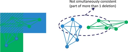
The final category of algorithms is based on deletion inference from genotype data with a familial structure. These SNP-based methods use genotype data to probe for specific genomic inheritance events that suggest inherited or de novo deletion polymorphisms. The key insight lies within inheritance patterns where an individual should be heterozygous for a SNP allele according to the laws of Mendelian inheritance, but is not. The deletion inference method employed here, as well as previously published methods (Conrad et al., 2006; McCarroll et al., 2006), relies on the fact that the SNP calling algorithm for SNP arrays and sequence data cannot distinguish between an individual who is homozygous for some allele a and an individual who has a deletion haplotype and the allele a (Fig. 1). Hemizygous deletions can then be inferred by finding such genotypic events throughout the data and analyzing their relationships to each other.
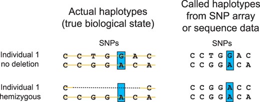
Alleles in the genomic interval of a hemizygous deletion are interpreted as homozygous by modern technologies. For example, individual 1 is correctly called heterozygous at the blue SNP position in the absence of a deletion but, if individual 1 is hemizygous, then each SNP will be called homozygous throughout the span of the deletion. This is true for SNP array (the intensities of only one probe is processed) and high-throughput sequencing technologies (sequence reads are sampled from a single chromosome).
Previously developed SNP-based methods were applied to HapMap data (International HapMap Consortium, 2003) containing a considerably fewer number of individuals than current GWAS data (albeit with more SNPs). These methods do not consider multiple individuals and thus have difficulties inferring recurrent deletions that may be associated with disease in association study data. However, SNP-based algorithms extend to genome-wide data and are not restricted to operate on SNP arrays; on the contrary, they have higher power to infer deletions from SNP calls on high-throughput sequencing data. Another considerable benefit of these approaches is that they are largely orthogonal to deletion inference from intensity- and sequence-based methods and can hence be used in conjunction with those methods to control type I and type II error.
1.3 Prior work on genome-wide deletion maps
Several algorithms exist capable of producing genome-wide deletion maps. McCarroll et al., 2006 developed a combinatorial clustering approach to identify sets of aberrant genotype inheritance patterns for dense genome-wide HapMap data. Conrad et al., 2006 first classifies SNP genotypes into several categories of Mendelian inheritance. They then iterate over all individuals separately and search for several sites that provide strong evidence of a deletion near each other. Both of these algorithms consider a single individual during deletion inference, which is effective at finding large deletions. However, these algorithms are underpowered when considering data containing small recurrent deletions. Corona et al., 2007 developed an algorithm aiming to support recurrent deletion calling by estimating haplotype frequencies assuming the presence or absence of a deletion in a window. This algorithm, however, phases the data first and the Mendelian inconsistencies caused by genomic deletions create difficulties for haplotype phasing algorithms. In fact, haplotype phasing algorithms generally convert all Mendelian inconsistencies to missing data prior to phasing thereby removing the deletion signal from the data. We presented an algorithm in Halldórsson et al., 2011 that called deletions based on a maximum clique finding heuristic algorithm. Although the run-time of this algorithm was acceptable for GWAS data, we found it was missing deletion calls in genomic regions of complex deletion signature. All of these methods employ heuristics and can miss small deletions that may be conserved among a few individuals in the sample.
Aside from algorithms that exclusively use SNP data, a number of different technologies have been used to determine deletions and other copy number variations (CNVs) throughout the human genome. Conrad et al., 2009 used tiling arrays to identify 8888 (7075 unique) CNVs. Park et al., 2010 employed a combination of a tiling array and resequencing to determine CNVs in an Asian population. Levy et al., 2007 identified a number of CNVs from the sequencing of a single individual. The 1000 Genomes Project has worked on identifying CNVs from the sequencing of a subset of one thousand individuals (Siva, 2008). There have also been SNP arrays developed to specifically target CNVs (Halldórsson and Gudbjartsson, 2011). These methods represent orthogonal analyses and can be used alongside SNP-based methods to infer deletions.
1.4 The DELISHUS approach
In this article, we present a SNP-based algorithmic framework for genome-wide hemizygous deletion inference termed DELISHUS (deletions in shared haplotypes using SNPs). We model the input SNP data using graph theory and implement efficient and exact algorithms to call genomic deletions based on biological conservation of a pattern of Mendelian inconsistency. Since our algorithms consider all individuals in the sample simultaneously, they achieve significantly lower false-positive rates and higher power when compared to previously published algorithms. By slightly modifying the model, we also present an algorithm for detecting de novo deletions. After deletions are called, we employ a similar graph theoretic approach for computing the critical regions of recurrent deletions in polynomial time. We also present a human genome deletion map of the Autism Genetic Resource Exchange (AGRE) GWAS data (Supplementary Fig. S1). Our algorithmic strategy is based on a combination of (i) using deletion conservation across many individuals to benefit from recurrent deletions in the population, (ii) modeling the input with graph theory and bounding the number deletion calls by a polynomial, and (iii) implementing an exact backtracking algorithm which completes its computation on a GWAS sized dataset in a few minutes due to a sparsity condition in the data. These three stringent requirements provide a rigorous basis for extracting genomic deletions of all sizes from the abundant SNP data available from high-throughput sequencing and array technologies.
2 METHODS
We organize the methods section around three computational biology problems for inferring deletions in genomes that present a signature of small recurrent deletions inspired by the genetics of autism.
Problem 1: identification of inherited deletions,
Problem 2: identification of de novo deletions and
Problem 3: identification of the critical regions of recurrent deletions
The DELISHUS algorithmic framework provides efficient and exact solutions to each problem.
2.1 Input and definitions
The input to our algorithm is an m×n genotype matrix M. The rows of M correspond to sets of related individuals and we assume that for every individual i there exists at least one other individual j such that i and j share a haplotype. In practice, M frequently consists of parent–child pairs or parents–child trios from a family-based association study design. The columns of M correspond to SNP calls for the m individuals. The genotype data are commonly obtained with SNP arrays but are increasingly acquired from whole-exome or whole-genome sequence data that provide SNP calls at a high resolution; consequently, this allows the detection of smaller or less frequent deletions.
Mendelian inheritance patterns in M can be divided into three major categories (Fig. 2). If an inheritance pattern can be explained only by the introduction of a deletion haplotype or a SNP call error, then we call it evidence of deletion. If the pattern can be explained by introducing a deletion haplotype or SNP call error but follows the laws of normal Mendelian inheritance, then we call it consistent with a deletion. Finally, if the pattern cannot be explained by introducing an inherited deletion haplotype then we call it no deletion.
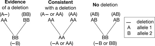
Each trio inheritance pattern can be classified into three categories under the interpretation of inherited deletions. The evidence of deletion pattern provides evidence for the presence of an inherited deletion. The no deletion pattern provides evidence for the absence of a deletion. The consistent with a deletion pattern does not provide strong evidence for the presence or absence of a deletion.
2.2 Problem 1: identification of inherited deletions
We assume, for ease of exposition, M consists of trio data. DELISHUS first converts M to a new matrix M′ with m/3 rows and n columns. Each row of M′ corresponds to a trio and each column corresponds to a trio-SNP inheritance pattern. Let the value of the (i,j) cell be denoted M′i,j. Then M′i,j∈{0,1,X} where
M′i,j=1 if the ith trio exhibits an evidence of deletion inheritance pattern at SNP j,
M′i,j=0 if the ith trio exhibits a consistent with a deletion inheritance pattern at SNP j and
M′i,j=X if the ith trio exhibits a no deletion inheritance pattern at SNP j.
DELISHUS then constructs a graph G(V,E) based on M′. A node is introduced for each evidence of deletion site and an edge between two nodes signifies that both nodes can be explained by the same deletion; formally, let vi,j denote the vertex associated with row i and column j, then vi,j∈V if M′i,j=1 and (vi,j,vk,l)∈E if the ranges [M′i,j,M′i,l] and [M′k,l,M′k,j] contain no X. In this graph, two nodes that are connected can be explained by the same deletion polymorphism and are termed compatible. Therefore, dense subgraphs of G correspond to genomic regions that are likely to contain inherited deletions. However, this picture is complicated by the fact that deletions may occur in a region of the genome independently and at slightly different intervals. Each vertex in G may be a member of many different dense subgraphs and thus we formulate the problem of identifying deletions as follows:
Formulation
For each connected component d∈G and for each set of vertices that form a maximal clique C in d, report C as deleted if |C|≥k where k is some threshold of evidence. Report a subset of vertices in C as genotyping errors if they are not members of at least one deletion.
In the absence of genotyping or sequencing errors, each evidence of deletion site would indicate a hemizygous deletion. In real data, random errors create false positives and the threshold k is tuned to lift predictions above the noise level by enforcing a minimum number of evidence of deletion sites to commit to a deletion. In particular, the value for k is guided by false-positive rate and power analysis experiments specifically tuned for a specific dataset. Formulation 1 computes all maximal cliques which, in G, correspond to rectangular areas of M′ whose evidence of deletion sites reinforce each other. It takes exponential time to compute and output all maximal cliques in a general graph; however, G has a special structure that allows us to achieve polynomial time algorithms.
lemma 1.
G contains at most  maximal cliques.
Proof.
Let C be a set of vertices forming a maximal clique in G. Let the interval of C be IC as defined by the span of SNPs from the leftmost evidence of deletion site of C (denoted l) to the rightmost evidence of deletion site of C (denoted r). We say C induces the interval of SNPs IC.
Since C is maximal, there cannot exist a vertex v ∉ C such that v is compatible with every vertex of C, thus IC cannot be extended. Furthermore, a maximal clique distinct from C but inducing IC cannot exist because each of its vertices must be compatible in the interval [l,r], which is in violation of the maximality of C. It follows that no maximal clique other than C can induce IC; thus, each maximal clique uniquely defines an interval. Since  distinct intervals exist for any given M′, the statement follows. ▪
Figure 3 gives an illustration of Lemma 1 on an example M′ and G.
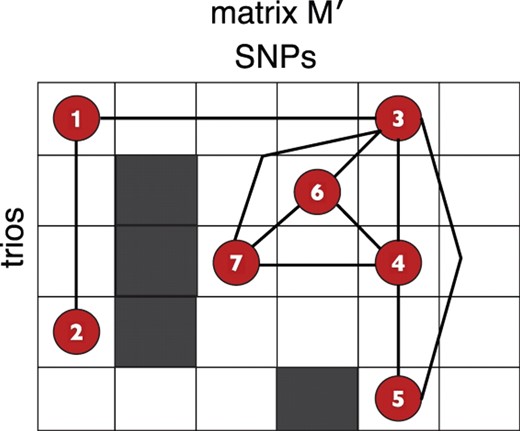
The outline of the matrix M′ is given with the red vertices corresponding to evidence of deletion sites in G. Four maximal cliques are formed, namely, {1,2},{1,3},{3,4,5} and {3,4,6,7}. Each maximal clique induces an interval that is the shortest such interval associated to the vertex set.
 . But, if non-overlapping sections of the matrix exist, we consider connected components separately; let di be the ith connected component of the set of all components D and ndi be the number of columns with at least one 1 in the SNPs of di.
We call the matrix M′ sparse if the number of connected components is large. A sparse M′ allows for trivial parallelization of deletion inference on distinct connected components and efficient computations due to the component sizes being small. Table 1 shows that the probability of evidence of deletion sites is low whereas the probability of a no deletion site is high for the HapMap and AGRE data. This suggests that M′ contains few deletion intervals compared to non-deleted intervals and thus M′ is sparse and D is large. This follows the intuition that the emergence of deletion polymorphisms are typically infrequent events.
The probabilities of an evidence of deletion site and a no deletion site for HapMap and autism GWAS data suggest M′ is sparse
| Data | Evidence of deletion | No deletion |
|---|---|---|
| HapMap P1 | 5.89×10⁻⁴ | 0.30 |
| HapMap P2+3 | 2.78×10⁻⁴ | 0.18 |
| AGRE autism | 1.21×10⁻⁴ | 0.41 |
| Data | Evidence of deletion | No deletion |
|---|---|---|
| HapMap P1 | 5.89×10⁻⁴ | 0.30 |
| HapMap P2+3 | 2.78×10⁻⁴ | 0.18 |
| AGRE autism | 1.21×10⁻⁴ | 0.41 |
Tsukiyama et al., 1977 presented an output sensitive algorithm that computes all maximal cliques of a component d with edges e in time O(de) per clique generated.
Corollary 1.
Computing all genomic deletions of M′ using Formulation 1 can be done in polynomial time.
In practice, however, the Bron–Kerbosch algorithm for maximal clique computation has proven to be more efficient. The Bron–Kerbosch algorithm is a recursive backtracking algorithm that computes all maximal cliques in an undirected graph but is not guaranteed to run in polynomial time. Although the Bron–Kerbosch algorithm is not an output-sensitive algorithm, it is still widely considered the fastest maximal clique finding algorithm (Cazals and Karande, 2008; Harley, 2004). Also, through empirical observations, the components of G are chordal with high probability. When a component of G is chordal, we can compute all maximal cliques even faster by simply generating a perfect elimination ordering.
With complex genetic heterogeneity (e.g. compound heterozygosity of small deletions), it is likely most informative to compute all possible configurations of deletions. Each maximal clique can be tested for association to disease if the data has a special structure. For example, the AGRE autism dataset includes families with a mixture of children diagnosed with autism and children without the disorder treated as healthy controls. DELISHUS computes the deletion transmission rates of parents to children with autism and parents to children whom are healthy; these deletion calls and transmission rates can be used to prioritize variants based on a number of statistical tests. This extra phenotypic information helps resolve situations where multiple deletion configurations are possible in the data (Fig. 4) and guides the deletion calls towards disease relevancy.
M′ is shown on the left with a superimposition of evidence of deletion vertices and edge connections. On the right, two maximal cliques are shown that share a subset of evidence of deletion sites. If the threshold k≤5, DELISHUS would report both cliques as potential deletions.
Formulation 1 also enables the resolution of complex genomic deletion ‘hot-spot’ regions. These regions (e.g. 22q11.21) pose the difficult problem of sorting through many possible configurations of deletions. DELISHUS can identify and process every deletion separately to resolve these complexity regions. Using this formulation, we called inherited deletions from the AGRE autism GWAS data and produced a high-level deletion map of autism (Supplementary Fig. S1). Table 2 demonstrates that DELISHUS is capable of efficiently resolving these regions for genome-wide data.
We ran DELISHUS using Formulation 1 on HapMap P1, P2+3 and the AGRE autism data
| Data | Runtime (s) | Memory (GB) |
|---|---|---|
| HapMap P1 CEU | 71.5 | <1 |
| HapMap P2+3 CEU | 91 | <1 |
| AGRE autism | 139.8 | 1.6 |
| Data | Runtime (s) | Memory (GB) |
|---|---|---|
| HapMap P1 CEU | 71.5 | <1 |
| HapMap P2+3 CEU | 91 | <1 |
| AGRE autism | 139.8 | 1.6 |
The HapMap P1 CEU data consists of 90 genotypes with about 1 million SNPs. The HapMap P2+3 CEU data consists of 174 genotypes with about 4 million SNPs. The AGRE data includes 4327 genotypes with about 500 thousand SNPs. We show DELISHUS scales to current GWAS sized data by presenting the runtime and memory requirements for the AGRE autism data. We ran DELISHUS on each chromosome in parallel on a cluster of 23 nodes. The numbers reported are the maximum requirements for a single machine in the computing cluster.
However, if evidence of deletion sites must be committed to exactly zero or one deletion, we can iteratively remove the largest clique of all maximal cliques in the component. More precisely, if the cardinality of a maximal clique is ≥k, we call the associated intervals deleted and remove the corresponding vertices from the graph. Statistical models that score deletions based on other quantities, such as deletion length or allele frequencies, may be used to provide a different ordering for the maximal clique processing. For example, if deletion length were the most important statistic, the green clique in Figure 4 would be preferable to the blue clique. This procedure is iterated until each evidence of deletion site has been called as part of a deletion or a SNP calling error.
2.3 Assessing the false-positive rate
Our algorithm uses enrichment of compatible evidence of deletion sites from many individuals to infer deletions. While inherited deletions are certainly a cause for evidence of deletion sites, these sites may also arise from genotyping or sequencing errors. To assess the false-positive rate occurring from random error, we computed the distribution of evidence, consistent and no deletion sites across three datasets: HapMap Phase 1 CEU, HapMap Phase 2+3 CEU and the AGRE autism data. We simulated a chromosome of length 25 000 SNPs with 30, 58 and 2500 parent–child trios for the HapMap Phase 1, HapMap Phase 2+3 and AGRE autism data, respectively. The inheritance patterns are drawn independently at random according to the distribution defined by each dataset. We ran this simulation at different thresholds for 1000 iterations. These computations are conservative because the evidence of deletion probabilities were computed from the entirety of the data including sites that may arise from both SNP calling errors and true genomic deletions.
The false-positive rate depends on the density of the SNP array, the sample size of trios and the probabilities of Mendelian inheritance patterns. In the HapMap data, DELISHUS produces very few false positives at a threshold of 3. In the larger AGRE autism data, DELISHUS requires a threshold of 5 to produce similar false-positive rates. In contrast, when DELISHUS is tuned to reproduce the results of Conrad et al., 2006 by considering each individual independently (identified as the single individual algorithm), a thresholds of 2 and 3 yields similar false-positive rates for both the HapMap and autism data. Table 3 summarizes these computations.
We simulated 25000 independent and identically distributed trio inheritance patterns according to the distribution observed in the data
| T | D P1 | D P2+3 | D AGRE | SI P1 | SI AGRE |
|---|---|---|---|---|---|
| 2 | 8.528 | 10.356 | 1214.063 | 0.701 | 1.854 |
| 3 | 0.076 | 0.135 | 141.13 | 0.001 | 0.001 |
| 4 | 0 | 0.001 | 11.274 | 0 | 0 |
| 5 | 0 | 0 | 0.632 | 0 | 0 |
| 6 | 0 | 0 | 0.028 | 0 | 0 |
| 7 | 0 | 0 | 0 | 0 | 0 |
| T | D P1 | D P2+3 | D AGRE | SI P1 | SI AGRE |
|---|---|---|---|---|---|
| 2 | 8.528 | 10.356 | 1214.063 | 0.701 | 1.854 |
| 3 | 0.076 | 0.135 | 141.13 | 0.001 | 0.001 |
| 4 | 0 | 0.001 | 11.274 | 0 | 0 |
| 5 | 0 | 0 | 0.632 | 0 | 0 |
| 6 | 0 | 0 | 0.028 | 0 | 0 |
| 7 | 0 | 0 | 0 | 0 | 0 |
The HapMap P1 CEU, P2+3 CEU and AGRE autism data were simulated with 30, 58 and 2500 trios, respectively. We inferred deletions using different thresholds (T) for DELISHUS (D) and the single individual (SI) algorithms. The statistic calculated for the false-positive rate is the average amount of deletions detected in 1000 iterations for the HapMap Phase 1 (P1), Phase 2+3 (P2) and AGRE autism GWAS data.
It is difficult to simulate false positives that may arise from technical artifacts, SNPs that are poorly genotyped, or SNPs that are undersampled from sequence reads. If such a SNP passes quality control (QC), we may detect the error by observing the distribution of Mendelian errors. Mendelian errors can be placed into two categories: those that show evidence of a deletion and those that do not. We assume there is no bias toward producing genotyping errors in either category. Even though evidence of deletion Mendelian errors are more probable, we would still expect to find non-evidence of deletion Mendelian errors for poorly genotyped SNPs. For these reasons, we may filter out SNP sites with many non-evidence of deletion Mendelian errors to reduce false-positive rates from systematic errors. Conservative approaches may further filter deletions that feature only one SNP containing evidence of deletion sites regardless of the Mendelian error distribution.
2.4 Estimating statistical power
The power to correctly infer deletions is a function of three variables: (i) the number of probes, distance between probes or size of the deletion; (ii) the frequency of the deletion in the population; and (iii) the allele frequencies. To estimate the power for predicting deletions, we use the HapMap Phase 1 CEU, Phase2+3 CEU and AGRE autism data; this selection fixes the allele frequencies. When computing the size of the deletion in base pairs, we select a genomic position at random and extend this interval for the defined size of the deletion. Therefore, it is possible for smaller deletions to be missed by the data completely if no SNPs exist within the deleted interval. We can also compute the size of a deletion in SNPs for which we randomly select a SNP and extend the deletion interval appropriately. In this case, there is always at least 1 SNP in the interval of the deletion. We varied the sizes of the deletions between 1 bp and 1 Mb or 1 and 20 SNPs and randomly selected three individuals in the HapMap data and five individuals in the AGRE autism data to harbor the deletions. To simulate the deletion, the genotypes of the child and a randomly selected parent were altered to indicate an inherited deletion. That is, the alleles of the child and selected parent were changed to homozygous for the non-transmitted allele in the span of the deletion. A deletion is said to be detected if the algorithm correctly reports a deletion for that specific trio. For example, if DELISHUS detects three individuals having a deletion within the simulated deleted region in the AGRE autism data, it will have detected 3/5 of the deletion.
We tested the power of the DELISHUS algorithm to detect inherited deletions within simulated intervals of various sizes in the HapMap P2+3 CEU data (Fig. 5A). In general, algorithms that infer deletions from SNP data have reduced power if only one parent is genotyped. This is also true of X chromosome deletions compared to the autosomes; the SNP calls for deleted haplotypes are less predictable and usually result in missing data. However, it is still feasible to call X chromosome deletions passed from mother to daughter. Due to the density of the data, our algorithm can robustly detect small deletions in the autosomes and performs fairly well on the X chromosome of females.
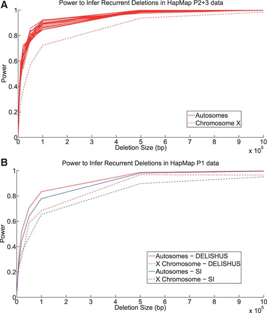
(A) The power to infer deletions in the HapMap Phase 2+3 CEU data as a function of the number of base pairs in the deletion. (B) We compare the power of the DELISHUS and single individual algorithms on HapMap Phase 1 CEU data. We average the power over all autosomes as they produced a similar curve. There is less power to predict deletions on chromosome X due to the male having only a single X chromosome. This power calculation was repeated 100 times for each autosome and then averaged. In both figures, the threshold of the DELISHUS algorithm was set to 3 and calibrated using the false-positive rate calculations of the previous section. Also a total of three individuals were selected at random to harbor the genomic deletion.
We then compare the power of the DELISHUS algorithm and the single individual algorithm for the HapMap P1 CEU data (Fig. 5B). This data is roughly one-quarter as dense but useful for comparison of smaller sample sizes; it is also the same data used by Conrad et al., 2006. There is a clear trade-off between false-positive rates and algorithmic power to detect deletions. However, when tuning the algorithms to achieve similar false-positive rates, the DELISHUS algorithm clearly outperforms the single individual algorithm due, in part, to leveraging the genomic information of the entire sample during inference.
Current association studies feature about as many SNPs as the HapMap data but many more individuals. Considering this, we applied the DELISHUS and single individual algorithms to the AGRE autism data (Fig. 6A). Five trios were selected at random (from the set of about 2500 trios) and a random interval was deleted. Using conservative thresholds, the DELISHUS algorithm is much more sensitive than the single individual algorithm. DELISHUS excels at inferring recurrent small deletions but the power of the two algorithms eventually converges as the deleted genomic interval increases. This proposition is highlighted in Fig. 6B where we inspect small deletions at a high resolution. The trend for the X chromosome is similar to the autosomes and is omitted.
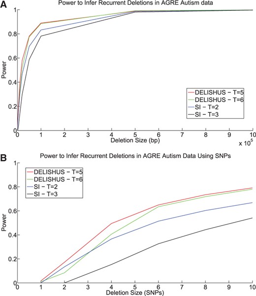
The power of the DELISHUS and single individual algorithms to infer inherited deletions in the AGRE autism autosomal data using (A) a view of large deletions defined by basepairs and (B) a higher resolution view for small deletions defined by SNPs. In both cases, a total of five individuals were chosen at random to harbor the deletion.
Power to infer deletions is also a function of deletion frequency. After increasing the frequency of the deletion in the sample from 0.2% to 1%, the power of the DELISHUS algorithm increases significantly and notably for smaller deletions (Fig. 7).
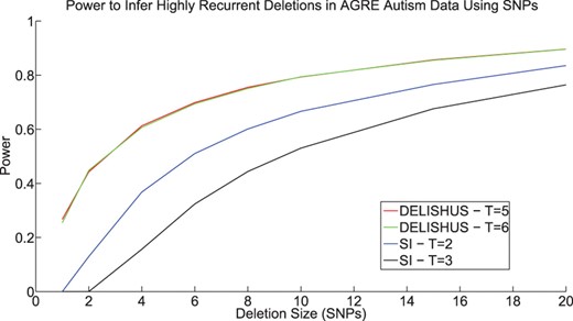
The power of the DELISHUS and single individual algorithms to infer highly recurrent small inherited deletions with a frequency of 1% (or 25 people) in the AGRE autism data.
2.5 Problem 2: identification of de novo deletions
Recent studies have highlighted the importance of protein altering de novo mutations for neural developmental disorders like autism (O'Roak et al., 2011). Inferring de novo deletions in genotype data is more difficult due to the parent having a lower frequency of homozygous SNPs over the interval of the child's deletion. For instance, the no deletion pattern in Fig. 2 could be hiding an undetectable de novo deletion. Figure 8 shows the inheritance patterns for inherited and de novo deletions for a pair of individuals sharing a haplotype. The most obvious relationship between the two types of deletions is that there is a much higher probability of consistent with a deletion patterns when inferring de novo deletions. This causes G to become more connected and, in regions of deletion complexity, may cause DELISHUS to run in superpolynomial time. However, Lemma 1 still applies, thus this problem remains theoretically polynomial and empirical evidence suggests our algorithms are still efficient.
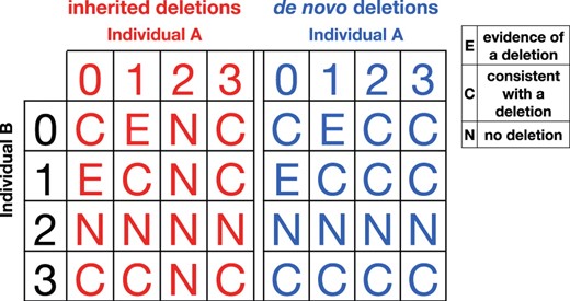
Categories of inheritance between a pair of individuals sharing a haplotype for inherited and de novo (in individual B) deletions. To represent all possible inheritance patterns, we encode an individual's SNP as 0 or 1 for the homozygote, 2 for the heterozygote and 3 for missing data. Unlike inherited deletions, if individual A is a heterozygote, individual B may still harbor a de novo deletion.
Table 4 shows false positive rates for the DELISHUS de novo deletion inference algorithm on the AGRE autism data. We do not observe a significant increase in the false positive rate because the probability of a no deletion site is only reduced slightly. If the probability of a no deletion site is high enough and the threshold is set to a large enough value, random genotyping errors cannot form enough compatible evidence of deletion sites to be called a deletion.
We simulated 25000 trio inheritance patterns for 2500 trios using parameters from the AGRE autism data
| T | D AGRE |
|---|---|
| 5 | 0.94 |
| 6 | 0.06 |
| 7 | 0.002 |
| T | D AGRE |
|---|---|
| 5 | 0.94 |
| 6 | 0.06 |
| 7 | 0.002 |
We inferred deletions using different thresholds (T) for the DELISHUS (D) de novo algorithm. The statistic calculated for the false-positive rate is the average amount of deletions detected in 500 iterations.
We have found many examples of de novo deletions in the autism AGRE dataset. Figure 9 shows the two different interpretations ofM′ using Figure 8. Due to data usage rules, we have substituted the gene name. It is certainly the case that one larger de novo deletion is more likely than three smaller inherited deletions. In this case, the de novo deletion becomes connected and not many other SNPs become consistent with a deletion. In practice, we do observe this same phenomenon.
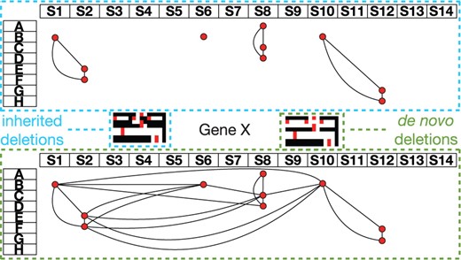
We show the graph G superimposed on M′ with the trio rows denoted A–H and the SNPs denoted S1–S14 for inherited and de novo deletion interpretations. For inherited deletions, Gene X displays three small 3-cliques each conferring little evidence of being a true deletion. When interpreting this data for de novo deletions, the second trio shows evidence for one larger de novo deletion. In G, we see that the second trio now becomes a hub for connections to trios C through F. The outlined black, red and white maps are deletion heat maps representing M′. Regions of 1's and 0's are represented by red and white, respectively. Regions of X's and 0's are represented by black.
2.6 Problem 3: identification of the critical regions of recurrent deletions
Deletions in autism and other neurological disorders are often recurrent (Stefansson et al., 2008; Weiss et al., 2008), with multiple deletions occurring in the same region of distinct individuals independently. Recurrently deleted regions often present a complex deletion signature with many deletions existing at slightly different intervals. While many configurations of deletions exist, interpretation of these regions is often formulated in a parsimonious manner. Critical regions capture this sense of parsimony and are defined as a region of large overlap for a subset of deletions. Critical regions are often used when attempting to connect a set of associated recurrent deletions to underlying biological mechanisms.
Since many critical regions may exist in the data, it is often useful to prioritize them by generating a ranking. Formulation 2 demonstrates one method for prioritization using critical region size.
Formulation 2.
Report all recurrently deleted regions shared by at least k′ deletions as significant critical regions.
To solve this formulation, we construct a graph G′(V′, E′) on the set of recurrent deletions. We introduce a vertex v∈V′ for each deletion and an edge (vi,vj)∈E′ if vi and vj share a SNP index. As the deletions are intervals on the chromosome, we can make the following observation.
Observation 1.
G′(V′,E′) is an interval graph and hence chordal.
Each maximal clique now corresponds to a critical region and its size corresponds to the number of deletions contained within the region. Therefore, an algorithm for Formulation 2 first computes G′(V′,E′) from the output of DELISHUS for inherited or de novo deletions. Since G′(V′,E′) is chordal, all critical regions are computed using perfect elimination orderings to generate maximal clique components in guaranteed polynomial time. Critical regions with the number of deletions ≥k′ are then ranked according to some metric (e.g. size).
2.7 Validation of deletions
Deletion calls may be validated with several types of experimental and computational methods. A select subset of deletions inferred in the autism GWAS data are scheduled to undergo experimental validation in Dr Morrow's laboratory using qPCR and custom-designed fine-tiling arrays. We validated our HapMap P1 deletion calls by comparing inferred inherited deletions to the deletions found by Conrad et al., 2006 and testing for a significant overlap. Conrad et al., 2006 developed a method that calls a region deleted if two or more evidence of deletion sites exist within close proximity to each other. From the set of computationally inferred deletion calls in the HapMap P1 data, they apply additional filtering steps and commit to 543 deletions (data extracted from the Database of Genomic Variants). From our analysis of the HapMap P1 data, we were able to produce a total of 1844 deletions covering all 543 deletions of Conrad et al., 2006.
We have shown previously that this type of analysis yields few false positives per chromosome (0.701 on average, Table 3). However, recurrent genomic deletions may be shared by descent or appear more frequently in specific genomic regions. In both cases, DELISHUS uses information of the entire sample to call genomic deletions that explains, in part, the increased number of deletion calls.
3 DISCUSSION
Using Formulation 1, DELISHUS computes all inherited or de novo deletions with maximal clique size above a user-defined threshold and then ranks them according to a number of different properties. Work in progress focuses on further validation studies and the prioritization of small recurrent deletions with the most support for experimental wet-lab validation in Dr Morrow's Laboratory. However, researchers may want to find deletions that are large and rare instead of small and recurrent. DELISHUS is adaptable to this type of inference by essentially mimicking the behavior of the Conrad et al., 2006 algorithm by restricting edges to within trio only. Furthermore, statistical rankings are also supported by this framework. After potential deletions are called, statistical and discrete quantities may be used to score and rank the deletions based on, for example, parent-of-origin effects which have been shown to be associated to autism (Arking et al., 2008; Fradin et al., 2010; Lamb et al., 2005) other examples of quantities to use for scoring include linkage disequilibrium, allele frequencies, size of deletion and number of evidence sites.
While we have found Formulation 1 to be the most useful, it only considers the case for which an error might convert a normal inheritance pattern to a 1. However, all potential conversions between deletion categories are possible (Fig. 10). Formulation 3 represents an alternative to Formulation 1, which models deletions and genotyping errors without the usage of a threshold.
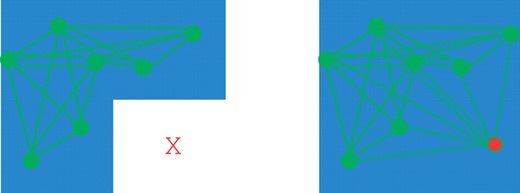
M′ is shown on the left with a superimposition of evidence of deletion vertices and edge connections. On the right, we demonstrate that making one X→1 correction unifies evidence of deletion sites into one larger deletion.
Formulation 3.
We are now allowed to correct any 1→X and any X→1 in M′. Find the minimum number of switches from 1→X or X→1 such that all cliques are disjoint.
Regardless of the formulation, there may still be other types of errors in SNP data such as technical artifacts producing completely erroneous SNPs. These are usually filtered in a preprocessing QC step, but it is often advantageous to allow DELISHUS to process the pre-QC data. For example, a small 1 SNP deletion that is associated to the phenotype of interest could mimic the behavior of a technical artifact and should not be removed prior to running DELISHUS.
As sequencing becomes cheaper and the sequencing of thousands of individuals becomes feasible, DELISHUS may prove to be a reliable source for calling small deletions genome-wide at a higher resolution than array data. For example, the 1000 Genomes Project is currently sequencing the genomes of HapMap individuals. Some of the HapMap individuals sequenced belong to parent–child trios and pairs. When this full sequence data becomes available, DELISHUS can be used on the SNP call data to validate previous calls in the HapMap data.
4 CONCLUSION
With increasingly dense SNP arrays and whole-exome sequencing becoming commonplace for studies of association, we are now ready for the genome-wide search for smaller deletion variants. Although the power of these newer technologies is enormous, genetic heterogeneity remains a daunting challenge and the identification of all polymorphism is paramount to the understanding of complex disease. While large genomic deletions have already been found and replicated, the problem of identifying small deletions remains an unmet challenge.
In this article, we presented three computational problems related to deletion inference in SNP data with a focus on small recurrent deletions in autism. We introduced the DELISHUS algorithmic framework for computing inherited deletions, de novo deletions and critical regions. Using a formulation inspired by the complexity of the deletion signature in autism, we showed that the problem of computing all inherited and de novo deletion configurations in SNP data can be solved in polynomial time (and empirically within minutes). We presented systematic methods to compute false-positive rates and power for the DELISHUS and single individual algorithms and demonstrated how to use the calculations to evaluate algorithmic performance and tune the threshold parameter. Comparisons of power, while controlling for false-positive rates, show that the DELISHUS algorithm excels at inferring small recurrent deletions. We also showed that finding critical regions of recurrent deletions may also be solved in polynomial time. The DELISHUS software package that implements these algorithms is readily available for download at the Istrail Lab website.
ACKNOWLEDGMENTS
Autism data is monitored by the laboratory of Eric Morrow as approved by institutional IRB. We gratefully acknowledge the resources provided by the AGRE Consortium and the participating AGRE families.
Funding: National Institute of Mental Health to Clara M. Lajonchere (PI) (Grant 1U24MH081810 to AGRE, partial); NIMH (1K23MH080954-05 to E.M.M.); Burroughs Wellcome Fund (to E.M.M., Career Award); National Science Foundation (Grant 1048831 to D.A., B.H. and S.I.)
Conflict of Interest: none declared.

