Integrating multi-OMICS data through sparse canonical correlation analysis for the prediction of complex traits: a comparison study

Abstract

Motivation

Recent developments in technology have enabled researchers to collect multiple OMICS datasets for the same individuals. The conventional approach for understanding the relationships between the collected datasets and the complex trait of interest would be through the analysis of each OMIC dataset separately from the rest, or to test for associations between the OMICS datasets. In this work we show that integrating multiple OMICS datasets together, instead of analysing them separately, improves our understanding of their in-between relationships as well as the predictive accuracy for the tested trait. Several approaches have been proposed for the integration of heterogeneous and high-dimensional (⁠$p\gg n$⁠) data, such as OMICS. The sparse variant of canonical correlation analysis (CCA) approach is a promising one that seeks to penalize the canonical variables for producing sparse latent variables while achieving maximal correlation between the datasets. Over the last years, a number of approaches for implementing sparse CCA (sCCA) have been proposed, where they differ on their objective functions, iterative algorithm for obtaining the sparse latent variables and make different assumptions about the original datasets.

Results

Through a comparative study we have explored the performance of the conventional CCA proposed by Parkhomenko et al., penalized matrix decomposition CCA proposed by Witten and Tibshirani and its extension proposed by Suo et al. The aforementioned methods were modified to allow for different penalty functions. Although sCCA is an unsupervised learning approach for understanding of the in-between relationships, we have twisted the problem as a supervised learning one and investigated how the computed latent variables can be used for predicting complex traits. The approaches were extended to allow for multiple (more than two) datasets where the trait was included as one of the input datasets. Both ways have shown improvement over conventional predictive models that include one or multiple datasets.

Availability and implementation

https://github.com/theorod93/sCCA.

Supplementary information

Supplementary data are available at Bioinformatics online.

1 Introduction

Nowadays, it is becoming a common practice to produce multiple OMICS (e.g. Transcriptomics, Metabolomics, Proteomics, etc.) datasets from the same individuals (Hasin et al., 2017; Hass et al., 2017; TCGA, 2012) leading to research questions involving the in-between relationships of the datasets as well as with the complex traits (responses). The datasets obtained through different mechanisms lead to different data distributions and variation patterns. The statistical challenge is how can these heterogeneous and high-dimensional datasets be analysed to understand their in-between relationships. A follow up question to address is how can these relationships be used for understanding the aetiology of complex traits.

Over the past years, a number of data integration approaches have been proposed for finding in-between dataset relationships (Li et al., 2018; Sathyanarayanan et al., 2019; Subramanian et al., 2020; Wu et al., 2019). These approaches can be split by their strategy: (A) Early: combining data from different sources into a single dataset on which the model is built; (B) Intermediate: combining data through inference of a joint model; and (C) Late: building models for each dataset separately and combining them to a unified model (Gligorijević and Pržulj, 2015). Huang et al. (2017) present a review of available methods for data integration and argue the need for direct comparisons of these methods for aiding investigators choosing the best approach for the aims of their analysis. A number of data integration approaches have been proposed in the literature for clustering disease subtypes (Mariette and Villa-Vialaneix, 2018; Swanson et al., 2019), whereas only few approaches have been proposed for supervised learning, i.e. for predicting the disease outcome (Jiang et al., 2016; Zhao et al., 2015). Van Vliet et al. (2012) investigated early, intermediate and late integration approaches by applying nearest mean classifiers for predicting breast cancer outcome. Their findings suggest that multiple data types should be exploited through intermediate or late integration approaches for obtaining better predictions of disease outcome.

The focus of this paper is on canonical correlation analysis (CCA), an intermediate integrative approach proposed by Hotelling (1936). CCA and its variations have been applied in various disciplines, including personality assessment (Sherry and Henson, 2005), material science (Rickman et al., 2017), photogrammetry (Vestergaard and Nielsen, 2015), cardiology (Jia et al., 2019), brain imaging genetics (Du et al., 2018, 2019) and single-cell analysis (Butler et al., 2018).

In the case of integrating two datasets CCA produces two new sets of latent variables, called canonical (variate) pairs. Suppose that there are two datasets with measurements made on the same samples (⁠$X_1\in {\mathbb{R}}^{n\times p_1}$ and $X_2\in {\mathbb{R}}^{n\times p_2}$⁠, assuming w.l.o.g. $p_1>p_2$⁠). For every ith pair, where $i=1,\dots ,\min (p_1,p_2)$⁠, CCA finds two canonical vectors, ${\mathbf{w}}_i^{(1)}$ and ${\mathbf{w}}_i^{(2)}$⁠, such that $\text{Cor}(X_1{\mathbf{w}}_i^{(1)},X_2{\mathbf{w}}_i^{(2)})$ is maximized based on the constraints described below. For the first pair, the only constraint to satisfy is $\text{Var}(X_1{\mathbf{w}}_1^{(1)})=\text{Var}(X_2{\mathbf{w}}_1^{(2)})=1$⁠. In computing the rth canonical pair, the following three constraints need to be satisfied:

1. $\mathit{\text{Var}}(X_1{\mathbf{w}}_r^{(1)})=\mathit{\text{Var}}(X_2{\mathbf{w}}_r^{(2)})=1$⁠.

2. $\mathit{\text{Cor}}(X_1{\mathbf{w}}_c^{(1)},X_1{\mathbf{w}}_r^{(1)})=\mathit{\text{Cor}}(X_2{\mathbf{w}}_c^{(2)},X_2{\mathbf{w}}_r^{(2)})=0,\hspace{1em}\forall c=1,\dots ,r-1$⁠.

3. $\mathit{\text{Cor}}(X_1{\mathbf{w}}_c^{(1)},X_2{\mathbf{w}}_r^{(2)})=\mathit{\text{Cor}}(X_2{\mathbf{w}}_c^{(2)},X_1{\mathbf{w}}_r^{(1)})=0,\hspace{1em}\forall c=1,\dots ,r-1$⁠.

Orthogonality among the canonical variate pairs must hold: that is, not just between the elements of each feature space, but also among all combinations of the canonical variates; except the ones in the same pair, for which the correlation must be maximized. Complete orthogonality is attained when these constraints are satisfied.

In other words, CCA finds linear combinations of X₁ and X₂ that maximize the correlations between the members of each canonical variate pair (⁠$X_1{\mathbf{w}}_i^{(1)},X_2{\mathbf{w}}_i^{(2)}$⁠), where $X_1{\mathbf{w}}_i^{(1)}=w_{i1}^{(1)}{X}_{11}+\cdots +w_{i{p}_1}^{(1)}{X}_{1p_1}$ and $X_2{\mathbf{w}}_i^{(2)}=w_{i1}^{(2)}{X}_{21}+\cdots +w_{i{p}_2}^{(2)}{X}_{2p_2}$⁠. By assuming that there exists some correlation between the datasets, we can look at the most expressive elements of canonical vectors (and indirectly, features) to find relationships between datasets.

CCA can be considered as an extension of principal component analysis (PCA) applied on two datasets rather than one dataset. Similarly to PCA, CCA can be applied for dimension reduction purposes, as the maximum size of the new sets of latent variables is $k=\min \{p_1,p_2\}$⁠.

A solution to CCA can be obtained through singular value decomposition (Hsu et al., 2012). The canonical vector ${\mathbf{w}}_i^{(1)}$ is an eigenvector of ${\Sigma }_{X_1{X}_1}^{-1}{\Sigma }_{X_1{X}_2}{\Sigma }_{X_2{X}_2}^{-1}{\Sigma }_{X_2{X}_1}$⁠, while ${\mathbf{w}}_i^{(2)}$ is proportional to ${\Sigma }_{X_2{X}_2}^{-1}{\Sigma }_{X_2{X}_1}{\mathbf{w}}_i^{(1)}$⁠. Each pair i of canonical vectors corresponds to the respective eigenvalues in a descending order.

In the case of high-dimensional data (⁠$p\gg n$⁠), the covariance matrix is not invertible and a CCA solution cannot be obtained. Over the years, a number of different methods have been proposed in the literature for finding solutions to this problem. These variations are called sparse CCA (sCCA) methods.

In recent years, several sCCA methods have been proposed, using different approaches, formulations and penalizations. Chu et al. (2013) implemented a trace formulation to the problem, Waaijenborg et al. (2008) applied Elastic-Net, while Fang et al. (2016) used a general fused lasso penalty to simultaneously penalize each individual canonical vector and the difference of every two canonical vectors. Other authors proposed methods based on sparse partial least squares. Lê Cao et al. (2009) assume symmetric relationships between the two datasets, Hardoon and Shawe-Taylor (2011) focus on obtaining a primal representation for the first dataset, while having a dual representation of the second, and the method proposed by Mai and Zhang (2019) that does not impose any sparsity on the covariance matrices.

In this paper, three sCCA methods that share similar characteristics in their formulation and optimizing criteria are discussed, investigated and extended. The first method, penalized matrix decomposition CCA (PMDCCA) proposed by Witten and Tibshirani (2009) obtains sparsity through l₁ penalization, widely known as least absolute shrinkage and selection operator (LASSO; Tibshirani, 1996). The bound form of the constraints is used in order to reach a converged solution by iteratively updating ${\mathbf{w}}^{(1)}$ and ${\mathbf{w}}^{(2)}$⁠. One of the assumptions of the PMDCCA approach is that the two datasets are independent, i.e. the covariance matrix of each input dataset is assumed to be the identity matrix. The second method proposed by Suo et al. (2017) relaxes the assumption of independence by allowing dependent data to be analysed through proximal operators [for the rest of the article, we are referring to this method as RelPMDCCA (relaxed PMDCCA)]. Even though, the additional restrictions make RelPMDCCA practically more applicable, it is computationally more expensive than PMDCCA. The third sCCA method we investigated is conventional CCA (ConvCCA) proposed by Parkhomenko et al. (2009). Similarly to PMDCCA sparsity is obtained through l₁ penalization. ConvCCA estimates the singular vector of $X_1^T{X}_2$ while iteratively applies the soft-thresholding operator. Chalise and Fridley (2012) extended ConvCCA to allow for other penalty functions and through a comparative study found the smoothly clipped absolute deviation (SCAD) penalty to produce the most accurate results. Motivated by this finding, in our work we have modified both ConvCCA and RelPMDCCA to be penalized through SCAD.

Section 2 starts with a description of the three sCCA approaches: PMDCCA, RelPMDCCA, ConvCCA, followed by a description of our proposed extension of ConvCCA and RelPMDCCA to allow for multiple input datasets. A comprehensive simulation study has been conducted for comparing the performance of the three methods and their extensions on integrating two and multiple datasets. To our knowledge, a comparison of the three sCCA methods has not been made elsewhere. The simulated datasets and scenarios considered are presented in Section 3.1.

We have further addressed the second important question; how can data integration be used for linking the multi-OMICS datasets with complex traits/responses? For addressing this question, we have looked the problem as both a supervised and an unsupervised one. For the supervised model, we have used the computed canonical pairs as input predictors in regression models for predicting the response. On the flip side, we have explored adding the response vector as an input matrix in the setting of multiple datasets integration. We have found both these approaches to have a better predictive accuracy than conventional machine learning methods that use either one or both of the input datasets. Section 4 presents the analysis of real datasets with the aim of predicting traits through sCCA.

2 Materials and methods

All sCCA methods share a common objective function, given by:

$${\text{min}}_{{\mathbf{w}}^{(1)},{\mathbf{w}}^{(2)}}-\text{Cor}(X_1{\mathbf{w}}^{(1)},X_2{\mathbf{w}}^{(2)})+p_{{\tau }_{w_1}}({\mathbf{w}}^{(1)})+p_{{\tau }_{w_2}}({\mathbf{w}}^{(2)}),$$

(1)

where $p_{{\tau }_{w_1}}({\mathbf{w}}^{(1)})$ and $p_{{\tau }_{w_2}}({\mathbf{w}}^{(2)})$ represent penalty functions on ${\mathbf{w}}^{(1)}$ and ${\mathbf{w}}^{(2)}$⁠, respectively. It is a bi-convex optimization where, if ${\mathbf{w}}^{(1)}$ is fixed, then Equation (1) is strictly convex in ${\mathbf{w}}^{(2)}$ and vice versa. Hence, one can find a solution through an iterative algorithm.

In this section, the computation of the first canonical pair is presented. To derive additional pairs, we have extended an approach proposed by Suo et al. (2017), which is presented in Section 2.6.

2.1 Conventional CCA

Parkhomenko et al. (2009) proposed a solution of sCCA based on approximating the sample correlation matrix and applying l₁ penalization through the soft-thresholding operator proposed by Tibshirani (1996). An iterative procedure updates both canonical vectors, ${\mathbf{w}}^{(1)}$ and ${\mathbf{w}}^{(2)}$⁠, at each iteration k. The procedure is illustrated in the following steps where one of the vectors (e.g. ${\mathbf{w}}^{(1)}$⁠) is updated while the second (e.g. ${\mathbf{w}}^{(2)}$⁠) is kept fixed: where $S({(w_l^{(1)})}^{k+1},\frac{1}{2}{\tau }_{w_j})={\left(\left|{(w_l^{(1)})}^{k+1}\right|-\frac{1}{2}{\tau }_{w_j}\right)}_{+}\text{Sign}({(w_l^{(1)})}^{k+1})$ and

$${(x)}_{+}=\{\begin{array}{cc}\mathrm{x}\hfill & \text{if} x\ge 0\hfill \\ 0\hfill & \text{if} x<0\hfill \end{array},\text{Sign}(x)=\{\begin{array}{cc}-1\hfill & \text{if} x<0\hfill \\ 0\hfill & \text{if} x>0\hfill \\ 1\hfill & \text{if} x=0\hfill \end{array},\forall l=\left\{1,\dots ,p_1\right\}$$

${\tau }_{w_j}$ represents the tuning parameter for each dataset Xj (j = 1, 2) and ${({\mathbf{w}}^{(1)})}^k$ is the value of ${\mathbf{w}}^{(1)}$ at the kth iteration. To update ${\mathbf{w}}^{(2)}$⁠, the same procedure is followed with the difference of replacing the second step with ${({\mathbf{w}}^{(2)})}^{k+1}\leftarrow K_{12}^T{({\mathbf{w}}^{(1)})}^{k+1}$⁠.

1. Compute sample correlation matrix $K_{12}={\Sigma }_{X_1{X}_1}^{-\frac{1}{2}}{\Sigma }_{X_1{X}_2}{\Sigma }_{X_2{X}_2}^{-\frac{1}{2}}$

2. ${({\mathbf{w}}^{(1)})}^{k+1}\leftarrow K_{12}{({\mathbf{w}}^{(2)})}^k$

3. Normalize ${({\mathbf{w}}^{(1)})}^{k+1}=\frac{{({\mathbf{w}}^{(1)})}^{k+1}}{\left|\right|{({\mathbf{w}}^{(1)})}^{k+1}\left|\right|}$

4. Apply soft-thresholding: ${(w_l^{(1)})}^{k+1}=S({(w_l^{(1)})}^{k+1},\frac{1}{2}{\tau }_{w_1})$

5. Normalize ${({\mathbf{w}}^{(1)})}^{k+1}=\frac{{({\mathbf{w}}^{(1)})}^{k+1}}{\left|\right|{({\mathbf{w}}^{(1)})}^{k+1}\left|\right|}$⁠,

2.2 Penalized matrix decomposition CCA

Witten and Tibshirani (2009) formulated the problem as:

$$\begin{array}{c}{\text{min}}_{{\mathbf{w}}^{(1)},{\mathbf{w}}^{(2)}}-\text{Cor}(X_1{\mathbf{w}}^{(1)},X_2{\mathbf{w}}^{(2)})+{\tau }_{w_1}\left|\right|{\mathbf{w}}^{(1)}|{|}_1+{\tau }_{w_2}|\left|{\mathbf{w}}^{(2)}\right|{|}_1\\ \text{subject} \text{to} \left|\right|{\mathbf{w}}^{(1)}|{|}_2\le 1;|\left|{\mathbf{w}}^{(2)}\right|{|}_2\le 1\end{array}.$$

(2)

An iterative algorithm based on penalized matrix decomposition (PMD) is applied with the update formula:

$${\mathbf{w}}^{(i)}\leftarrow \frac{S(X_i^T{X}_j{\mathbf{w}}^{(j)},{\Delta }_i)}{\left|\right|S(X_i^T{X}_j{\mathbf{w}}^{(j)},{\Delta }_i)|{|}_2},$$

(3)

where ${\Delta }_i>0$ is chosen such that $\left|\right|{\mathbf{w}}^{(i)}|{|}_1=1$ holds, or ${\Delta }_i=0$ if $\left|\right|{\mathbf{w}}^{(i)}|{|}_1\le 1$⁠, for $i,j=1,2,\hspace{0.17em}i\ne j$⁠. Although the PMDCCA solution is different from the ConvCCA solution, both approaches assume that the features are independent within each dataset (i.e. $X_i^T{X}_i=I_{p_i},i=1,2$⁠).

2.3 Relaxed PMDCCA

Suo et al. (2017) proposed a solution that relaxes the independence assumption and applies penalization through proximal operators. Their formulation of the problem is similar to (2):

$$\begin{array}{c}{\text{min}}_{{\mathbf{w}}^{(1)},{\mathbf{w}}^{(2)}}-\text{Cor}(X_1{\mathbf{w}}^{(1)},X_2{\mathbf{w}}^{(2)})+{\tau }_{w_1}\left|\right|{\mathbf{w}}^{(1)}|{|}_1+{\tau }_{w_2}|\left|{\mathbf{w}}^{(2)}\right|{|}_1\\ \text{subject} \text{to} \text{Var}(X_1{\mathbf{w}}^{(1)})\le 1;\text{Var}(X_2{\mathbf{w}}^{(2)})\le 1\end{array}.$$

(4)

The solution to this optimization is obtained through linearized alternating direction method of multipliers (Boyd, 2010; Parikh and Boyd, 2014). The iterative updates on the canonical variate pairs are computed through proximal algorithms. Due to space limitations, to view the updates, we refer the readers to the original paper by Suo et al. (2017).

2.4 Implementing SCAD penalty

The SCAD (Fan and Li, 2001) penalty with tuning parameter τ applied on w is given as follows:

$$p_{\tau }^{\text{SCAD}}(w)=\{\begin{array}{ll}\tau \left|\right|w|{|}_1\hfill & \text{if }\left|\right|w|{|}_1\le \tau \hfill \\ -\frac{\left|\right|w|{|}_1^{\mathrm{2}}-2a\tau |\left|w\right|{|}_1+{\tau }^2}{2(a-1)}\hfill & \text{if }\tau <\left|\right|w|{|}_1\le a\tau \hfill \\ \frac{(a+1){\tau }^2}{2}\hfill & \text{if }\left|\right|w|{|}_1>a\tau \hfill \end{array}$$

(5)

where a is fixed and suggested by Fan and Li to be set as a = 3.7. Motivated by the findings of Chalise and Fridley (2013), we have modified RelPMDCCA to perform penalization through SCAD.

Even though SCAD is a non-convex penalty function, Mazumder et al. (2011) argue that if the optimizing function is strictly convex, then penalization via SCAD is well-behaved and converges to a stationary point. In the objective functions of ConvCCA [Equation (1)] and RelPMDCCA [Equation (4)], ${\tau }_{w_1}\left|\right|{\mathbf{w}}^{(1)}|{|}_1+{\tau }_{w_2}|\left|{\mathbf{w}}^{(2)}\right|{|}_1$ is replaced by $p_{{\tau }_{w_1}}^{\mathit{SCAD}}({\mathbf{w}}^{(1)})+p_{{\tau }_{w_2}}^{\mathit{SCAD}}({\mathbf{w}}^{(2)})$⁠. As a result the iterative updates of the canonical vectors are different. In ConvCCA, the algorithm is adjusted accordingly by replacing the soft-thresholding operator in Step 4 with:

$${(w_l^{(1)})}^{i+1}=\{\begin{array}{cc}{(|{(w_l^{(1)})}^{i+1}|-{\tau }_{w_1})}_{+}\text{Sign}({(w_l^{(1)})}^{i+1})\hfill & \text{if} \left|{(w_l^{(1)})}^{i+1}\right|\le 2{\tau }_{w_1}\hfill \\ \frac{(a-1){(w_l^{(1)})}^{i+1}-\text{Sign}({(w_l^{(1)})}^{i+1})a{\tau }_{w_1}}{a-2}\hfill & \text{if} 2{\tau }_{w_1}<\left|{(w_l^{(1)})}^{i+1}\right|\le a{\tau }_{w_1}\hfill \\ {(w_l^{(1)})}^{i+1}\hfill & \text{if} {(w_l^{(1)})}^{i+1}>a{\tau }_{w_1}\hfill \end{array}.$$

(6)

The updates of canonical vectors in RelPMDCCA with SCAD penalty are performed by:

$$\mathbf{p}\mathbf{r}\mathbf{o}{\mathbf{x}}_{\mu f}({\omega }_j)=\{\begin{array}{cc}{\omega }_j+\mu c_j-\mu {\tau }_{w_1}\hfill & \text{if} \mu {\tau }_{w_1}<{\omega }_j+\mu c_j\le {\tau }_{w_1}+\mu {\tau }_{w_1}\hfill \\ {\omega }_j+\mu c_j=+\mu {\tau }_{w_1}\hfill & \text{if}-{\tau }_{w_1}-\mu {\tau }_{w_1}\le {\omega }_j+\mu c_j<-\mu {\tau }_{w_1}\hfill \\ \frac{{\omega }_j+\mu c_j-\mu {\eta }_2}{1+2\mu {\eta }_1}\hfill & \text{if} {\psi }_1+\mu {\eta }_2<{\omega }_j+\mu c_j\le a{\psi }_1+\mu {\eta }_2\hfill \\ \frac{{\omega }_j+\mu c_j+\mu {\eta }_2}{1+2\mu {\eta }_1}\hfill & \text{if}-a{\psi }_1-\mu {\eta }_2\le {\omega }_j+\mu c_j<-{\psi }_1-\mu {\eta }_2\hfill \\ {\omega }_j+\mu c_j\hfill & \text{if} |{\omega }_j+\mu c_j|>a{\tau }_{w_1}\hfill \\ 0\hfill & \text{else}\hfill \end{array},$$

(7)

where ${\eta }_1=-\frac{1}{2(a-1)},\hspace{0.17em}{\eta }_2=\frac{2a{\tau }_{w_1}}{2(a-1)},\hspace{0.17em}{\psi }_1={\tau }_{w_1}(1+2\mu {\eta }_1),\hspace{0.17em}c=X_1^T{X}_2{\mathbf{w}}^{(2)}$ and $\mathit{\omega }=({({\mathbf{w}}^{(1)})}^k-\frac{\mu }{\lambda }(X_1^T(X_1{({\mathbf{w}}^{(1)})}^k-{\mathbf{z}}^k+{\mathit{\xi }}^k)))$⁠. The parameter ${\tau }_{w_1}$ controls the sparseness level while the algorithm parameters μ and λ must satisfy $0<\mu \le \frac{\lambda }{\left|\right|X_1|{|}_2^2}$ (Parikh and Boyd, 2014). ${\mathbf{w}}^{(2)}$ is updated through the same proximal operators, with ${\tau }_{w_2}$ acting as the tuning parameter. The update functions of z and $\mathit{\xi }$ remain the same.

2.5 Multiple sCCA

In OMICS studies, it is common for a study to have more than two datasets (such as transcriptomics, genomics, proteomics and metabolomics) on the same patients. Incorporating all available data simultaneously through an integrative approach can reveal unknown relationships between the datasets. This section presents extensions of the three sCCA methods we have seen, for the integration of multiple (more than two) datasets simultaneously.

Suppose we have M separate datasets denoted by $X_1,\dots ,X_M$⁠, where $X_m\in {\mathbb{R}}^{n\times p_m},\hspace{0.17em}\forall m=\{1,\dots ,M\}$⁠. The problem of Equation (1) is then generalized as:

$${\text{min}}_{w^{(1)},\dots ,w^{(M)}}{\displaystyle \sum _{i<j}-}\text{Cor}(X_i{w}^{(i)},X_j{w}^{(j)})+{\displaystyle \sum _{m=1}^M{p}_{{\tau }_{w_m}}}(w_m)$$

(8)

As sCCA is bi-convex, multiple sCCA is multi-convex, i.e. if ${\mathbf{w}}^{(j)},\hspace{0.17em}\forall j\ne i$ are fixed, then the problem is convex in ${\mathbf{w}}^{(i)}$⁠. Instead of producing maximal correlated canonical variate pairs (2-tuple), multiple sCCA produces canonical variate list (M-tuple), e.g. for $i=1,\dots ,\min (p_1,\dots ,p_M)$⁠, the ith canonical variate list would be (⁠$X_1{\mathbf{w}}_i^{(1)},\dots ,X_M{\mathbf{w}}_i^{(M)}$⁠). Each $X_m{\mathbf{w}}^{(m)}$ is taken such that, it is maximally correlated with the rest of the latent features $\sum _{j\ne m}{X}_j{\mathbf{w}}^{(j)}$⁠.

In multiple ConvCCA, we propose to update ${\mathbf{w}}^{(i)}$ iteratively, by keeping ${\mathbf{w}}^{(j)},\hspace{1em}\forall j\ne i$ and computing $K_{ij},\hspace{1em}\forall j\ne i$⁠. On the kth iteration, ${\mathbf{w}}^{(i)}$ is updated by ${({\mathbf{w}}^{(i)})}^{k+1}\leftarrow \sum _{j\ne i}{K}_{ij}{({\mathbf{w}}^{(i)})}^k$ (Algorithm 1 in Supplementary Material).

Witten and Tibshirani (2009) proposed an extension to their solution, by assuming that $X_m^T{X}_m=I_{p_m},\hspace{1em}\forall m=\left\{1,\dots ,M\right\}$⁠. To update ${\mathbf{w}}^{(i)}$⁠, the canonical vectors ${\mathbf{w}}^{(j)}, \forall j\ne i$ are kept fixed. Multiple PMDCCA can then be performed by minimizing ${\mathbf{w}}^{{(i)}^T}{X}_i^T\left(\sum _{j\ne i}{X}_j{\mathbf{w}}^{(j)}\right), \forall i=\{1,\dots ,M\}$⁠, with constraint functions $\left|\right|{\mathbf{w}}^{(m)}|{|}_2\le 1$⁠.

We have extended RelPMDCCA for multiple datasets by following the approach of PMDCCA. The constraint functions $\text{Var}(X_m{\mathbf{w}}^{(m)})\le 1, \forall m=(1,\dots ,M)$ and the proximal operators remain the same. If ${\mathbf{w}}^{(j)}\hspace{1em}\forall j\ne 1$ are kept fixed, we can update ${\mathbf{w}}^{(1)}$⁠, by replacing $-{\mathbf{w}}^{{(1)}^T}{X}_1^T{X}_2{\mathbf{w}}^{(2)}$ in Equation (4) with $-{\mathbf{w}}^{{(1)}^T}{X}_1^T\sum _{j\ne 1}{X}_j{\mathbf{w}}^{(j)}$⁠.

The tuning parameters in sCCA and multiple sCCA are selected as the ones producing maximal correlation through cross-validation. A detailed description of the procedure is presented in the Supplementary Material.

In this work, we have explored the performance of the methods in predicting the response of interest when the response is included as one of the datasets being integrated.

2.6 Computing the additional canonical vectors

We have only addressed the computation of the first canonical variate pair so far but this might not be adequate for capturing the variability of the datasets and of their relationships. Similarly to PCA as the number of computed principal components is increased the total amount of variability explained is increased. By computing the additional canonical vectors of CCA additional constraints must be satisfied as illustrated below.

Suo et al. (2017) compute the remaining canonical vectors by adding the second constraint to the optimization. Let $W_1=({\mathbf{w}}_1^{(1)},\dots ,{\mathbf{w}}_{r-1}^{(1)})$ and $W_2=({\mathbf{w}}_1^{(2)},\dots ,{\mathbf{w}}_{r-1}^{(2)})$ define the r - 1 canonical vectors which were computed. The rth canonical vector of ${\mathbf{w}}^{(1)}$ is found through the optimization problem:

$$\begin{array}{c}{\text{min}}_{{\mathbf{w}}^{(1)}}-{\mathbf{w}}^{{(1)}^T}{X}_1^T{X}_2{\mathbf{w}}^{(2)}+p_{{\tau }_{w_1}}({\mathbf{w}}^{(1)})+1\{{\mathbf{w}}^{(1)}:|\left|X_1{\mathbf{w}}^{(1)}\right|{|}_2\le 1\}\\ \text{subject} \text{to} W_1^T{X}_1^T{X}_1{\mathbf{w}}^{(1)}=0\end{array},$$

(9)

where $p_{{\tau }_{w_1}}({\mathbf{w}}^{(1)})$ and $p_{{\tau }_{w_2}}({\mathbf{w}}^{(2)})$ represent the penalty functions on ${\mathbf{w}}^{(1)}$ and ${\mathbf{w}}^{(2)}$ with parameters ${\tau }_{w_1}$ and ${\tau }_{w_2}$⁠, respectively. This solution would successfully result in producing latent features that are uncorrelated within the new datasets of canonical vectors, although the correlation is not restricted between the two new datasets.

In an attempt to include the additional constraint to the optimization problem, we propose the following extension to Equation (9):

$$\begin{array}{c}{\text{min}}_{{\mathbf{w}}^{(1)}}-{\mathbf{w}}^{{(1)}^T}{X}_1^T{X}_2{\mathbf{w}}^{(2)}+p_{{\tau }_{w_1}}({\mathbf{w}}^{(1)})+1\{{\mathbf{w}}^{(1)}:|\left|X_1{\mathbf{w}}^{(1)}\right|{|}_2\le 1\}\\ \text{subject} \text{to} X_1{\mathbf{w}}^{(1)}=\mathbf{z};W_1^T{X}_1^T\mathbf{z}=0_{r-1};W_2^T{X}_2^T\mathbf{z}=0_{r-1}\end{array}.$$

(10)

The solution to this optimization problem is obtained by letting $\tilde{X}=\left[\begin{array}{c}{X}_1\\ W_1^T{X}_1^T{X}_1\\ W_2^T{X}_2^T{X}_1\end{array}\right]$⁠, and $\tilde{Y}=\left[\begin{array}{c}Y\\ W_2^T{X}_2^T{X}_2\\ W_1^T{X}_1^T{X}_2\end{array}\right]$⁠. The rth canonical vector is then computed by applying an sCCA method on $\tilde{X}$ and $\tilde{Y}$ to obtain ${\mathbf{w}}_r^{(j)},\hspace{1em}j=1,2$⁠, respectively. The exact algorithm in computing the additional canonical vectors is presented in Algorithm 2 in Supplementary Material.

Witten and Tibshirani (2009) proposed to update the cross-product matrix $Y=X_1^T{X}_2$ after the computation of each canonical pair, by $Y^{j+1}\leftarrow Y^j-({\mathbf{w}}_j^{{(1)}^T}{Y}^j{\mathbf{w}}_j^{(2)}){\mathbf{w}}_j^{(1)}{\mathbf{w}}_j^{{(2)}^T}$⁠, where ${\mathbf{w}}_j^{(1)}$ and ${\mathbf{w}}_j^{(2)}$ are the jth canonical vectors. The authors of ConvCCA proposed to take the residual of K by removing the effects of the first canonical vectors and repeat the algorithm in order to obtain the additional canonical pairs.

3 Results

3.1 Simulation studies

Simulated datasets were generated for assessing the performance of the three methods on (i) integrating two datasets, (ii) the orthogonality attained by each method and (iii) integrating multiple datasets. PMDCCA was implemented by using the existing functions in R package $\mathit{PMA}$⁠. We used our own code for ConvCCA and RelPMDCCA, as they were not found publicly available; our code is available in the github link provided in the abstract.

3.1.1 Models, scenarios and evaluation measures

3.1.1.1 Models

Three models were used for simulating data with similar characteristics as OMICS datasets. All three data-generating models are based on five parameters, $n,p_1,p_2,p_1^{(cc)},p_2^{(cc)}$⁠, where n represents the number of samples, p_i is the total number of features in X_i and $p_i^{(cc)}$ represents the number of features in X_i which are cross-correlated with the rest of datasets (⁠$p_i^{(cc)}\le p_i$⁠). Different types of scenarios were examined covering a range of possible data characteristics. The data were generated based on the assumption of having high canonical correlation. Further, a separate null scenario was designed in which canonical correlation was taken to be low.

Simple model. A simple data-generating model that generates data for $M\ge 2$ datasets:

$$X_i=\mathbf{u}{\mathbf{w}}^{{(i)}^T}+{ϵ}_i,\hspace{1em}i=\left\{1,\dots ,M\right\},$$

(11)

where $\mathbf{u}\in {\mathbb{R}}^n,\hspace{0.17em}{\mathbf{w}}^{(i)}\in {\mathbb{R}}^{p_i}$ and ${ϵ}_{ij}\sim \mathcal{N}(0,1),\hspace{1em}j=1,\dots ,p_i$⁠. Only the first $p_i^{(cc)}$ elements of ${\mathbf{w}}^{(i)}$ are non-zero, representing the cross-correlated features that we seek to identify.

Single-latent variable model.  Parkhomenko et al. (2009) proposed a single-latent variable model in assessing ConvCCA. An extension of this model is presented here, allowing the generation of multiple datasets. M datasets, $X_m\in {\mathbb{R}}^{n\times p_m},m=\left\{1,\dots ,M\right\}$⁠, are generated, such that the first $p_m^{(cc)}$ features of each X_m would be cross-correlated. In other words, w.l.o.g. the first $p_m^{(cc)}$ of X_m will be correlated with the first $p_j^{(cc)}$ of $X_j,\forall j\ne m$⁠. These groups of features are associated with each other according to the same (single-latent variable) model. A latent variable, $w^{(i)}$⁠, explains a subset of observed variables in X_i, i.e. $\left\{X_{i,1},\dots ,X_{i,p_i^{(cc)}}\right\}$⁠. Through a common higher-level latent variable, μ, $\hspace{1em}{w}^{(i)}\hspace{1em}\forall i$⁠, are correlated. The rest of the features are independent within their respective datasets.

After simulating a random variable $\mu \sim \mathcal{N}(0,{\sigma }_{\mu }^2)$⁠, the data are generated as follows:

1. For the cross-correlated variables:${(x_m)}_{ij}={\alpha }_j^{(m)}{\mu }_i+e_{x_{m}ij}$ for $i=1,\dots ,n,\hspace{0.17em}j=1,\dots ,p_m^{(cc)},\hspace{0.17em}m=1,\dots ,M$where we assume $\sum _{i=1}^{}{\alpha }_i^{(m)}=1,\forall m$⁠, and $e_{x_{m}ij}\sim \mathcal{N}(0,{\sigma }_e^2),\hspace{1em}\forall i,j,m$⁠.

2. For the independent variables:${(x_m)}_{ij}=e_{x_{m}ij}$ for $i=1,\dots ,n,\hspace{0.17em}j=p_m^{(cc)}+1,\dots ,p_1,\hspace{0.17em}m=1,\dots ,M$ where again we assume $e_{x_{m}ij}\sim \mathcal{N}(0,{\sigma }_e^2),\hspace{1em}\forall i,j,m$⁠.

Fig. 1.

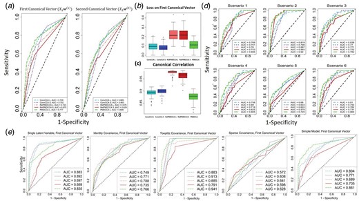
sCCA performance on simulated data for integrating two datasets. (a) ROC curve plots on all five sCCA methods after averaging over all data-generating models and all scenarios. (b) Box-plots of the overall loss of the first canonical vector (⁠$X_1{\mathbf{w}}^{(1)}$⁠) averaged over all data-generating models and scenarios, and (c) canonical correlation in the simulation studies for sCCA. (d) ROC curve plots, showing averaged results (over the models) for each scenario on $X_1{\mathbf{w}}^{(1)}$⁠. (Results on $X_2{\mathbf{w}}^{(2)}$ can be seen in the Supplementary Material). (e) ROC curve plots, showing averaged (over the scenarios) results for each model on $X_1{\mathbf{w}}^{(1)}$

Supplementary Figure S1 paints a picture of the single-latent variable data-generating model.

Covariance-based model.  Suo et al. (2017) proposed simulations based on the structure of the covariance matrices of both datasets (X1 and X2). Three types of covariance matrices were considered in this study: (i) Identity, (ii) Toeplitz and (iii) Sparse. We have utilized this model for generating two datasets. Details regarding this data-generating model can be found in Supplementary Material.

3.1.1.2 Scenarios and evaluation measures

In comparing the three sCCA methods for integrating two datasets, six scenarios of different data characteristics were examined (Table 1). The first scenario acts as a baseline for the rest. A single parameter is changed for each additional scenario. In addition to the six scenarios, a null scenario was implemented, at which the two datasets were generated through the covariance-based model with true canonical correlation, $\rho =0.1$⁠. The purpose of this null simulation model is to understand better how the methods work, and determine the likelihood of obtaining a high correlation by chance.

Table 1.

Data characteristics and simulation scenarios used to evaluate the three sCCA methods for integrating two or three datasets

Scenarios	Data characteristics
Integrating two datasets
Null	$n=100,1000,10000,\hspace{1em}{p}_1=80,\hspace{1em},p_2=60,\hspace{1em}{p}_1^{(cc)}=5,\hspace{1em}{p}_2^{(cc)}=15$
1	$n=40,\hspace{1em}{p}_1=80,\hspace{1em},p_2=60,\hspace{1em}{p}_1^{(cc)}=5,\hspace{1em}{p}_2^{(cc)}=15$
2	$n=150,\hspace{1em}{p}_1=80,\hspace{1em},p_2=60,\hspace{1em}{p}_1^{(cc)}=5,\hspace{1em}{p}_2^{(cc)}=15$
3	$n=40,\hspace{1em}{p}_1=200,\hspace{1em},p_2=60,\hspace{1em}{p}_1^{(cc)}=5,\hspace{1em}{p}_2^{(cc)}=15$
4	$n=40,\hspace{1em}{p}_1=80,\hspace{1em},p_2=200,\hspace{1em}{p}_1^{(cc)}=5,\hspace{1em}{p}_2^{(cc)}=15$
5	$n=40,\hspace{1em}{p}_1=80,\hspace{1em},p_2=60,\hspace{1em}{p}_1^{(cc)}=50,\hspace{1em}{p}_2^{(cc)}=15$
6	$n=40,\hspace{1em}{p}_1=80,\hspace{1em},p_2=60,\hspace{1em}{p}_1^{(cc)}=5,\hspace{1em}{p}_2^{(cc)}=50$
Integrating three datasets
1	$n=40,\hspace{1em}{p}_1=80,\hspace{1em},p_2=60,\hspace{1em}{p}_3=40,\hspace{1em}{p}_1^{(cc)}=15,\hspace{1em}{p}_2^{(cc)}=10,\hspace{1em}{p}_3^{(cc)}=5$
2	$n=40,\hspace{1em}{p}_1=200,\hspace{1em},p_2=60,\hspace{1em}{p}_3=40,\hspace{1em}{p}_1^{(cc)}=15,\hspace{1em}{p}_2^{(cc)}=10,\hspace{1em}{p}_3^{(cc)}=5$
3	$n=150,\hspace{1em}{p}_1=80,\hspace{1em},p_2=60,\hspace{1em}{p}_3=40,\hspace{1em}{p}_1^{(cc)}=15,\hspace{1em}{p}_2^{(cc)}=10,\hspace{1em}{p}_3^{(cc)}=5$

Note: n represents the number of samples, while $p_i^{(cc)}$ and p_i represent the cross-correlated and total number of features, respectively, in dataset i, for i = 1, 2.

We assessed the performance of the sCCA methods for integrating multiple datasets by generating three datasets through three scenarios as shown in Table 1.

The sCCA methods in both simulation studies were evaluated by measuring: (i) the canonical correlation; (ii) the correct identification of sparsity in the data, by computing accuracy, precision and recall of the true non-zero elements of the estimated canonical vectors; and (iii) the loss between true and estimated canonical vectors. A detailed description of the evaluation measures is presented in the Supplementary Material.

An additional simulation study was conducted to evaluate orthogonality. Two datasets were generated, with each of the following scenarios used in all three data-generating models: (i) $n=500,p_1=100,p_2=200,p_1^{(cc)}=20,p_2^{(cc)}=40$⁠, (ii) $n=150,p_1=100,p_2=200,p_1^{(cc)}=20,p_2^{(cc)}=40$ and (iii) $n=50,p_1=100,p_2=200,p_1^{(cc)}=20,p_2^{(cc)}=40$⁠.

3.1.2 Simulation outcomes

3.1.2.1 Integrating two datasets

In the conducted simulation study, the performance of sCCA methods was assessed on the three data-generating models and six scenarios shown in Table 1. The results are based on the first canonical pair.

Figure 1a depicts the resulting ROC curves and their area under the curve (AUC) values, averaged over all data-generating models and scenarios. ConvCCA with SCAD had the best performance in identifying correctly the sparseness and the non-zero elements of canonical vectors, as it produced the highest AUC. RelPMDCCA with SCAD obtained the lowest AUC value, which shows that the optimal choice of penalty function depends on the sCCA method. While the second dataset (and latent features $X_2{\mathbf{w}}^{(2)}$⁠) obtained slightly reduced sensitivity, the sCCA methods performed in a similar fashion as with the first dataset.

RelPMDCCA produced the highest loss between the true and estimated canonical vectors (Fig. 1b), but it also provided the highest canonical correlation (Fig. 1c). Its overall averaged correlation is close to 1, while for the other two methods, it is closer to 0.9.

Figure 1d shows the performance of the first canonical vector (⁠$X_1{\mathbf{w}}^{(1)}$⁠) averaged over all data-generating models. As expected, by increasing the number of samples in a case where n > p (Scenario 2), the AUC values on all sCCA increased, with RelPMDCCA showing the largest improvement. However, a decrease in the performance of all sCCA methods is observed when the number of non-zero elements is increased. This can be seen on Scenarios 5 and 6, for ${\mathbf{w}}^{(1)}$ and ${\mathbf{w}}^{(2)}$⁠, respectively. We can argue that in cases where the non-zero elements of a canonical vector are at least half of its length (total number of elements), the methods fail to correctly identify some of them. That might be due to the fact that sCCA methods force penalization and expect a sparser outcome. Furthermore, since the performance on ${\mathbf{w}}^{(2)}$ in Scenario 6 is worse than that on ${\mathbf{w}}^{(1)}$ in Scenario 5, we can argue that the higher the ratio of non-zero elements over the total number of elements, the less accurate the identification. On Scenarios 3 and 4, where the total number of features is increased while the non-zero elements are not, sCCA methods performed as well as on the baseline scenario.

After averaging over the scenarios, the methods’ performance on each data-generating model is shown in Figure 1e. The methods’ performance seems to be overall influenced by the choice of data-generating model. In the case of single-latent variable model, ConvCCA clearly produced the least errors, while in the simple model, PMDCCA produced the highest AUC values. In the covariance-based models, all sCCA methods performed equally well in estimating correctly non-zero elements of the canonical vectors. Methods on Toeplitz model produced higher AUC values than on Identity model, where Sparse model contained the most errors out of all data-generating models. Based on this observation, we can argue that the sparser the data, the less accurate the methods.

3.1.2.2 Null simulation model

To conclude our simulation study in integrating two datasets, we applied the three sCCA methods on two datasets, simulated to have low canonical correlation. Two datasets were generated by following the covariance-based model and setting the true correlation $\rho =0.1$ on different sample sizes, n = 100, 1000, 10 000. The rest of the simulation parameters remained constant as presented in Table 1.

As sample size increases, the correlations obtained by all methods are decreasing (Table 2). Even though the datasets were simulated to have low correlation, it is possible that a certain combination of their respective features could have high correlation by chance due to the small sample size. ConvCCA and RelPMDCCA captured this relationship and produced high canonical correlation on low-sampled simulations, while PMDCCA did a better a job in avoiding it even with n = 100. PMDCCA produced the highest AUC on simulations with small sample size, while on n = 10 000, RelPMDCCA captured the true non-zero features more accurately than PMDCCA and ConvCCA (Fig. 2).

Fig. 2.

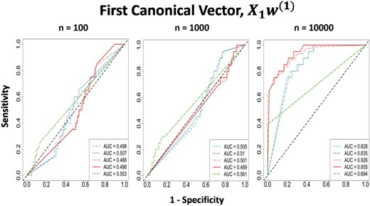
sCCA performance on Null scenario. ROC curves of the first canonical vector by all three sCCA on Null scenario with sample sizes n = 100, 1000, 10 000

Table 2.

Null simulation model

Canonical correlation on Null simulation model
	PMDCCA	ConvCCA	ConvCCA	RelPMDCCA	RelPMDCCA
Sample size	LASSO	LASSO	SCAD	LASSO	SCAD
n = 100	0.55 (0.08)	0.81 (0.05)	0.80 (0.02)	0.96 (0.05)	0.98 (0.02)
n = 1000	0.22 (0.03)	0.48 (0.02)	0.48 (0.04)	0.51 (0.01)	0.50 (0.02)
n = 10 000	0.12 (0.03)	0.26 (0.05)	0.24 (0.03)	0.26 (0.04)	0.26 (0.04)

Note: Canonical correlations of PMDCCA, ConvCCA and RelPMDCCA averaged across 100 runs on the null scenarios.

The results of this simulation, along with the results of Section 3.2.1, suggest that although ConvCCA and RelPMDCCA are capable in producing a larger canonical correlation than PMDCCA, the likelihood of that correlation being due to chance is greater. The same conclusions were reached after repeating this process on two independent and uncorrelated datasets.

3.1.2.3 Orthogonality and sparsity

A third simulation study was conducted, with the aim of evaluating orthogonality of the three sCCA methods. For each method, orthogonality was enforced differently. For RelPMDCCA the solution proposed in Section 2.6 was applied, while for ConvCCA and PMDCCA we applied the solutions proposed by Parkhomenko et al. (2009) and Witten and Tibshirani (2009), respectively.

The scenarios in this study are split into three cases, based on the data sparsity: (i) $n>p_2>p_1$⁠, (ii) $p_2>n>p_1$ and (iii) $p_2>p_1>n$⁠. Table 3 shows the classification of each case with one out of three classes: (A) Full (Orthogonality): all pairs were found to be orthogonal; (B) Partial: most, but not all pairs were found to be orthogonal; and (C) None: none, or limited pairs were found to be orthogonal. Different colours in Table 3 refer to the different simulation models: simple model, single-latent variable model, identity covariance-based model.

Table 3.

Orthogonality of sCCA methods

Orthogonality of all simulations with five canonical variates
Methods $->$	PMDCCA	ConvCCA	RelPMDCCA
$n>p_2>p_1$	None Orthogonality Partial Orthogonality Partial	Full Orthogonality Partial Full	Partial None None
$p_2>n>p_1$	None Partial Full	None None None	Full Full Partial
$p_2>p_1>n$	Full Full Full	None None None	Full Full Full

Note: The table shows whether the algorithms succeed in obtaining orthogonal pairs. None refers to not obtaining orthogonality at all; Full refers to obtaining orthogonality between all pairs; Partial for some, but not all. For each scenario, simulations via the simple simulation model, single-latent variable model and covariance-based model are represented by the first, second and third rows, respectively.

Table 4.

A summary on the performance of sCCA methods based on both the simulation studies conducted and the analysis of real data

Summary on the performance of sCCA methods
On two datasets	ConvCCA	Great performance on simulation studies, especially on single-latent model
		Over-fitted cancerTypes data and performed well on nutriMouse
		Low time complexity
	PMDCCA	Good performance on simulation studies, especially on simple model
		Over-fitted cancerTypes data and performed well on nutriMouse
		Low time complexity
	RelPMDCCA	Moderate to good performance on simulation studies
		Had the best performance in analysing two real datasets
		High time complexity
Multiple datasets	ConvCCA	Good performance on simulation studies
		Avoided over-fitting and improved performance in both data studies
		Low time complexity
	PMDCCA	Very good performance on simulation studies
		Avoided over-fitting and improved performance in both data studies
		Low time complexity
	RelPMDCCA	Moderate to good performance on simulation studies
		Overall obtained the best results in both data studies
		High time complexity

Note: It is an intuitive evaluation of the methods, split into having two datasets or multiple.

As summarized in Table 3, orthogonality is not always preserved, and that depends on the sCCA method, as well as on the data characteristics. The choice of data-generating model did not have a high impact in attaining orthogonality. All sCCA methods were penalized through l₁ during this simulation study.

In case (i), ConvCCA has attained full orthogonality on the first five canonical variate pairs, where PMDCCA and RelPMDCCA failed to do so (except between some pairs). In the other two cases, none of the canonical variates obtained from ConvCCA were orthogonal. PMDCCA preserved complete orthogonality in $p_2>p_1>n$ case and most when $p_2>n>p_1$⁠. Complete orthogonality was attained in both of those cases when RelPMDCCA was implemented. Parkhomenko et al. (2009) and Witten and Tibshirani (2009) only consider the first canonical pair in their examples and do not explicitly discuss the performance of their respective methods on additional canonical pairs.

3.1.2.4 Integrating three datasets

A simulation study on multiple sCCA was performed by generating three datasets through the (i) simple model and (ii) single-latent variable model. The same evaluating measures as with the case with the two datasets were computed. Canonical correlation was evaluated by computing the average canonical correlation of each dataset with the rest.

Figure 3a presents the averaged (arithmetic) canonical correlation observed by each method. RelPMDCCA produced the highest, as it did in with the case of two datasets. PMDCCA produced the least correlated and least sparse solution, suggesting that it is not performing very well with multiple datasets where the objective of sCCA is to maximize the correlation between the datasets. Figure 3b shows the sparsity obtained by each method with RelPMDCCA providing the sparsest solution.

Fig. 3.

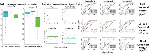
Multiple sCCA performance on simulated data for integrating three datasets. (a) Box-plots showing the canonical correlation along the ConvCCA, RelPMDCCA and PMDCCA methods in a multiple setting. (b) An example of a scatter plot for the first estimated canonical vector. (c) ROC curves on multiple sCCA simulations

Overall, PMDCCA produces the highest AUC values. RelPMDCCA was superior only when the number of samples was increased (Scenario 3). RelPMDCCA and ConvCCA showed a decrease in their performance when the number of non-zero elements was increased, but PMDCCA was able to maintain its good performance.

3.2 Real datasets

3.2.1 NutriMouse

Martin et al. (2007) have performed a nutrigenomic study, with gene expression (⁠$X_1\in {\mathbb{R}}^{n\times p_1}$⁠) and lipid measurements (⁠$X_2\in {\mathbb{R}}^{n\times p_2}$⁠) on n = 40 mice, with $p_1=120$ genes and concentrations of $p_2=21$ lipids were measured. Two response variables are available: diet and genotype of mice. Diet is a five-level factor: coc, fish, lin, ref, sun and genotype is recorded as either Wild-type (WT), or Peroxisome Proliferator-Activated Receptor-α (PPARα). NutriMouse data are perfectly balanced in both responses, in which an equal number of samples is available for each class.

Through the analysis of the nutriMouse datasets we aimed to (i) evaluate which of three considered sCCA approaches performs better and (ii) determine whether data integration of datasets can improve prediction over conventional approaches that only analyse a single dataset. For addressing the second question, we have implemented the following off the shelf statistical machine learning approaches: (A) Principal Components Regression (PCR)—logistic model with first 10 principal components acting as predictors; (B) Sparse Regression (SpReg)—penalized (through LASSO and SCAD) logistic and multinomial models, when the response was diet and genotype, respectively; (C) k-Nearest Neighbours (kNN) for supervised classification; and (D) k-means for unsupervised clustering—acting as a benchmark in splitting the data by ignoring the labels. Since two datasets are available, these four methods were implemented on the following three cases of input data: (i) only X₁, (ii) only X₂ and (iii) $X_{\text{both}}=(X_1,X_2)\in {\mathbb{R}}^{n\times p_{\text{both}}}$⁠, where $p_{\text{both}}=p_1+p_2$⁠. The aforementioned machine learning methods and the three sCCA approaches were applied on 100 bootstrap samples of the datasets, taking separate training and test sets at each repetition, for assessing the predictive accuracy of the methods. For the machine learning methods applied, the version with the input dataset obtaining the smallest error was compared with the sCCA approaches. In predicting the genotype response using only X₁ (i.e. gene expression data) was preferred, but X_both was chosen with diet acting as the response (Supplementary Material).

Figure 4 shows the predictive accuracy of the methods on both diet (Fig. 4a) and genotype (Fig. 4b). PCR and k-means were the least accurate methods (Supplementary Material). In predicting either response, sCCA methods outperformed the conventional machine learning methods. Both the sCCA approaches and the conventional machine learning approaches had very high accuracy for predicting the genotype response whereas their accuracy was lower for predicting the diet response. All the methods had an accuracy between 0.7 and 0.86, except RelPMDCCA that had the highest accuracy 0.92. The precision and recall measures showed similar patterns with RelPMDCCA obtaining the highest values for both measures against all other methods (Supplementary Material).

Fig. 4.

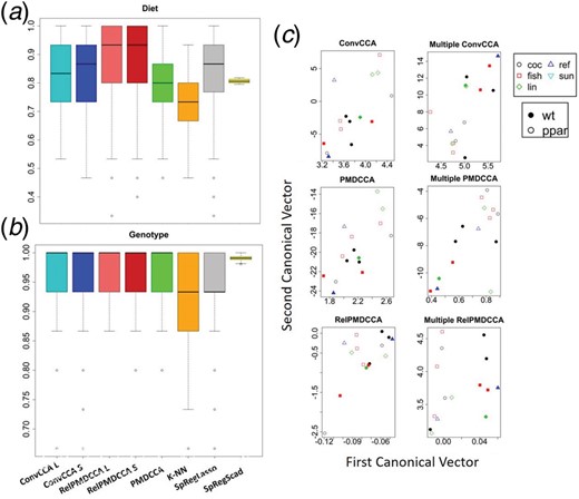
sCCA performance on nutriMouse data. Box-plots presenting the accuracy of sCCA methods, k-NN and SpReg with LASSO and SCAD with the response being (a) diet and (b) genotype. (c) Scatter plots of the canonical vectors from the first canonical variate pair of a random nutriMouse test set, after applying sCCA and multiple sCCA

Multiple sCCA with response matrix. We applied our proposed extensions of the sCCA approaches for multiple datasets, where one of the input datasets is the matrix of the two response vectors.

Figure 4c presents the canonical vectors of the first canonical variate pair. The first column of plots shows the canonical vectors obtained without considering a response matrix. On a two-setting integration, the data are not separated well for neither response. However, by including the response matrix, multiple sCCA methods separated clearly the samples between WT and PPARα mice, as shown in the second column of Figure 4c. A slight improvement in their separation between diets was also observed. All multiple sCCA methods performed equally well, although visually RelPMDCCA indicates the clearest separation in terms of genotype.

3.2.2 CancerTypes

Due to the abundance of data in the Cancer Genome Atlas (TCGA) database, a lot of researchers have applied various integrative algorithms for cancer research (Lock et al., 2013; Parimbelli et al., 2018; Poirion et al., 2018; Wang et al., 2014). Gene expression, miRNA and methylation data from three separate cancer types were taken: (i) breast, (ii) kidney and (iii) lung. For each patient, we also have information about their survival status. Thus, the goal of this analysis was to assess whether (multiple) sCCA can improve conventional classification methods in determining the cancer type, and survival status.

The data consist of 65 patients with breast cancer, 82 with kidney cancer and 106 with lung cancer, from which 155 patients are controls. The data in this study cover 10 299 genes (X₁), 22 503 methylation sites (X₂) and 302 mi-RNA sequences (X₃). Data cleaning techniques such as removing features with low gene expression and variance were used, leaving us with a remaining of 2250 genes and 5164 methylation sites. Similarly to Section 4.1, k-NN, PCR and SpReg were applied, along with sCCA algorithms. After investigating the best combination, miRNA expression and methylation datasets were selected for integrating two datasets. Multiple sCCA was implemented on all three available datasets.

Figure 5a presents the accuracy, precision and recall of each method in predicting the patients’ survival status. SpReg, ConvCCA and PMDCCA produced perfect recall, while their precision was recorded around 60%. Such finding suggests over-fitting as a single class is favoured. Thus, a solution providing good results while avoiding over-fitting would be preferable.

PCR and k-NN did not show any signs of over-fitting, but did not perform well (PCR had accuracy below 0.5 and k-NN had consistently low values on all three measures). RelPMDCCA did not over-fit the data and produced high measure values, especially with LASSO being the penalty function. Multiple RelPMDCCA produced the most accurate and precise solution out of all methods applied. Multiple PMDCCA and ConvCCA improved the results of their respective integration method on two datasets, as they avoided over-fitting, with precision and recall values being more balanced. Regardless of the response, same conclusions were reached, i.e. implementing multiple sCCA can avoid over-fitting.

Figure 5b presents the scatter-plots of the test set of the canonical vectors of the first canonical variate pair. In contrast with the nutriMouse study, visually there is no clear separation observed between cancer types or survival status of the patients. Since the objective of sCCA is to maximize canonical correlation, it is important to preserve it. The canonical vectors of the test set are computed by linearly combining the estimated canonical vectors (through training), with the original test datasets. RelPMDCCA produced the highest correlation in all three combinations of canonical vectors (Fig. 5b).

Fig. 5.

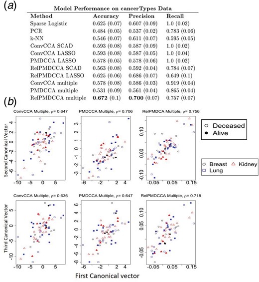
sCCA performance on cancerTypes data. (a) Model performance for the prediction of samples’ survival status. The best overall performed model is shown with bold. (b) Scatter-plots of canonical variates in cancerTypes analysis through multiple sCCA

4 Discussion

The increasing number of biological, epidemiological and medical studies with multiple datasets on the same samples calls for data integration techniques that can deal with heterogeneity and high-dimensional datasets.

Over the years, a lot of methods for sCCA have been proposed that integrate high-dimensional data. In this study, we have focused on ConvCCA, PMDCCA and RelPMDCCA, as these methods penalize the same optimizing function [Equation (1)]. We modified RelPMDCCA to penalize canonical vectors through SCAD and we compared its performance against LASSO penalty. Further, we proposed an extension in computing the additional canonical pairs. The extension satisfies necessary conditions in enforcing orthogonality among them. Finally, we extended ConvCCA and RelPMDCCA for integrating more than two datasets instead of just two as their original version.

By collectively reducing the dimensions of the datasets, while obtaining maximal correlation between the datasets, sCCA methods were found to have better accuracy in predicting complex traits than other conventional machine learning methods. Through our proposed extensions of the ConvCCA and RelPMDCCA approaches for integrating more than two datasets and for incorporating the response matrix as one of the integrated datasets, we have showed that over-fitting can be avoided and higher predictive accuracy can be obtained.

Through the analysis of the two real datasets, we illustrated that the sCCA methods can improve our predictions of complex traits in both cases: (i) when a regression model is built with the new canonical matrices as input matrices and (ii) when the response matrix is one of the input matrices in the data integration. For both cases, the sCCA methods can improve the predictions of the response.

Table 4 summarises our conclusions on each of the three sCCA methods applied on two or multiple datasets. Even though both nutriMouse and cancerTypes datasets have small sample sizes, the latter has a large number of features, providing an indication of a true genomic-wide scale analysis. We found that RelPMDCCA obtained the best results, but it is also more computationally expensive than the other methods. We conclude that in cases where datasets with large number of features or samples, PMDCCA might be a more appropriate method to consider due to its advantage regarding computational time. This observation calls for further optimizing RelPMDCCA in reducing its complexity and increasing its feasibility on large-scale analysis. The computation times of the methods are presented in the Supplementary Material.

Our simulation study findings are in agreement with Chalise and Fridley (2012) that showed that ConvCCA has better results with SCAD penalty rather than LASSO. When analysing two uncorrelated datasets both ConvCCA and RelPMDCCA had a greater likelihood of obtaining high correlation compared to PMDCCA, when the number of samples is small. With larger sample sizes, all methods obtained smaller correlations. With no exception, RelPMDCCA provides the highest canonical correlation in all simulation studies and all real-data analyses performed in this paper.

To preserve orthogonality, the results of our simulation study suggest different methods based on data characteristics. If the data satisfy $n>p_1>p_2$⁠, then ConvCCA is a more sensible choice. In the other cases (⁠$p_1>n>p_2$ or $p_1>p_2>n$⁠), ConvCCA failed to provide orthogonal canonical pairs, while PMDCCA and RelPMDCCA, attained orthogonality on synthetic data from all three data-generating models. We observed the performance of the sCCA methods to depend on the structure of the input data. For sparse datasets, we recommend the use of the RelPMDCCA approach as it is the one that performed better for such datasets.

Huang et al. (2017) argued the need for a comparison of data integration approaches. This paper has addressed this by evaluating the performance of three sCCA approaches. We have further illustrated that integrating datasets through multiple sCCA could improve the prediction power, suggesting that researchers with access to two or more datasets should aim for an integrative analysis.

Financial Support: none declared.

Conflict of Interest: none declared.

Acknowledgements

The authors would like to thank Sarah Filippi, Philipp Thomas and Takoua Jendoubi for useful conversations.