Sparse redundancy analysis of high-dimensional genetic and genomic data

Abstract

Motivation

Recent technological developments have enabled the possibility of genetic and genomic integrated data analysis approaches, where multiple omics datasets from various biological levels are combined and used to describe (disease) phenotypic variations. The main goal is to explain and ultimately predict phenotypic variations by understanding their genetic basis and the interaction of the associated genetic factors. Therefore, understanding the underlying genetic mechanisms of phenotypic variations is an ever increasing research interest in biomedical sciences. In many situations, we have a set of variables that can be considered to be the outcome variables and a set that can be considered to be explanatory variables. Redundancy analysis (RDA) is an analytic method to deal with this type of directionality. Unfortunately, current implementations of RDA cannot deal optimally with the high dimensionality of omics data (⁠$p\gg n$⁠). The existing theoretical framework, based on Ridge penalization, is suboptimal, since it includes all variables in the analysis. As a solution, we propose to use Elastic Net penalization in an iterative RDA framework to obtain a sparse solution.

Results

We proposed sparse redundancy analysis (sRDA) for high dimensional omics data analysis. We conducted simulation studies with our software implementation of sRDA to assess the reliability of sRDA. Both the analysis of simulated data, and the analysis of 485 512 methylation markers and 18,424 gene-expression values measured in a set of 55 patients with Marfan syndrome show that sRDA is able to deal with the usual high dimensionality of omics data.

Availability and implementation

http://uva.csala.me/rda.

Supplementary information

Supplementary data are available at Bioinformatics online.

1 Introduction

In the past, genetic and genomic data have often been associated with (disease) phenotypes on a variable by variable basis. Recently, however, there has been much interest in associating multiple phenotypes with multiple genetic and or genomic datasets (Ritchie et al., 2015). This area, often referred to as integromics (Lê Cao et al., 2009), aims to combine clinical and several molecular data sources (i.e. omics data) in an effort to find shared pathways that are involved in certain phenotypes. A typical research direction in integromics is often focused on explaining the variability in the phenotypes of an organism from various molecular data sources. The central dogma of molecular biology states that there is a sequential transfer of information within a biological organism (Crick, 1970). Thus, the DNA transcription variability can be explained from DNA structural variability and regulatory factors, and RNA to protein translation can be further explained by RNA levels and regulatory factors.

One of the main challenges in integromics is that the data sources often contain far more variables than observations, leading to multicollinearity. To solve this problem, Waaijenborg and Zwinderman (2009) and Witten and Tibshirani (2009), among others, proposed sparse Canonical Correlation Analysis (sCCA) to extract linear combinations from the data sources in such a way that these linear combinations are maximally correlated. A drawback of sCCA is that it is a symmetrical method and does not impose directionality, implying that it does not make a distinction between the variables that need to be predicted and the predictive variables. As a consequence, applying sCCA to explain the variability in the phenotypes from omics data sources has two disadvantages. Firstly, the symmetric process introduces unnecessary computational costs and leads to suboptimal computational time. Secondly, since the result is described in terms of highly correlated pairs (i.e. principal components) of linear combinations of variables from the two respective datasets involved [and it is possible that the highest correlated set of variables are found in the last principal component (Fornell et al., 1988)], the interpretability of the results is hampered (van den Wollenberg, 1977; Takane and Hwang, 2007).

As an alternative to CCA it is possible to use redundancy analysis (RDA), which is a well-known non-symmetric multivariate technique (Fornell et al., 1988; Johansson, 1981; Stewart and Love, 1968; van den Wollenberg, 1977). In RDA, a clear distinction is made between the predicted and predictive variables. By taking advantage of this directionality, the computational time is substantially lower than CCA. In addition, the main objective of RDA is to optimize the multivariate correlation coefficients between a linear combination of the predictive variables and the variables in the predicted dataset (Lambert et al., 1988; Takane and Hwang, 2007). Since the obtained regression weights will be equal with the correlation between the individual predictive variables and the predicted dataset, the results from RDA are easier to interpret than the results of CCA.

Takane and Hwang (2007) proposed regularized RDA based on introducing the Ridge penalty in RDA. Although this solves the multicolinearity problem, all the predictor variables will have a non-zero contribution, which hampers interpretation of the results if there are thousands or even millions of predictor variables.

To solve the interpretation problems of sparse RDA, we introduced the Elastic Net (ENet) penalty in the RDA framework. The ENet penalty is shown to perform better on datasets with high collinearity, which is often the case with omics data. To do this, we extended the two factor partial least squares model for RDA proposed by Fornell et al. (1988). In general, our tool provides a descriptive multivariate statistics tool for high dimensional omics data analysis that delivers easily interpretable results.

2 Materials and methods

2.1 Framework for redundancy analysis by Fornell

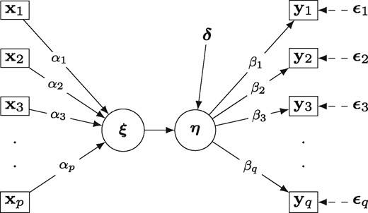
Consider we have observations on n individuals spread over $\mathbf{X}\in R^{n\times p}$ containing p explanatory (predictive) variables and $\mathbf{Y}\in R^{n\times q}$ containing q response (predicted) variables. It is assumed that all explanatory and response variables are standardized and normalized.

Let $\mathit{\xi }=\{{\xi }_i;i=1,\dots ,n\}$ be a unidimensional variate formed by a linear combination of the explanatory variables from X, i.e.

$${\xi }_i=\sum _{k=1}^p{x}_{ik}{\alpha }_k,$$

(1)

where $\mathit{\alpha }=\{{\alpha }_k;k=1,\dots ,p\}$ are the weights of the explanatory variables. The main goal of RDA is to determine $\mathit{\alpha }$ in such a way that the sum of absolute correlations between $\mathit{\xi }$ and each column from Y is maximized (Israëls, 1992), i.e.

$$arg\text{max}\sum _{k=1}^q\left|\mathit{\xi }{Y}_k\right|.$$

(2)

Fornell et al. (1988) proposed to estimate the weights $\mathit{\alpha }$ with a two factor partial least squares model (Fig. 1). To do this, we require an additional variate $\mathit{\eta }=\{{\eta }_i;i=1,\dots ,n\}$⁠, which is defined as

$${\eta }_i=\sum _{j=1}^q{y}_{ij}{\beta }_j,$$

(3)

where $\mathit{\beta }=\{{\beta }_k;k=1,\dots ,p\}$ are the weights of the outcome variables. The two factor partial least squares model is based on the following relations between the variates and the data in X and Y,

$$\begin{array}{cc}{\eta }_i\hfill & =\sum _{j=1}^q{x}_{ij}{\alpha }_j+{\delta }_i,\hfill \\ y_{ij}\hfill & ={\xi }_i{\beta }_j+{\mathrm{ϵ}}_{ij},\hfill \end{array}$$

(4)

where ${\mathrm{ϵ}}_{ij}\sim N(0,\sigma )$ and ${\delta }_i\sim N(0,\tau )$ are residual terms. The $\mathit{\alpha }$ weights can be interpreted as the contribution of the X variables to $\mathit{\xi }$⁠, and the $\mathit{\beta }$ values indicate the correlation between the particular Y variables and $\mathit{\xi }$⁠, the linear combination of the X variables.

Fig. 1.

The two factor partial least squares RDA model, proposed by Fornell et al. (1988)

Fornell showed that the weights $\mathit{\alpha }$ and $\mathit{\beta }$ can be estimated by iteratively performing traditional ordinary least squared (OLS) regressions. The estimation of $\mathit{\beta }$ involves the k = 1,…,q univariate OLS regressions

$${\mathit{\beta }}_k={\left({\mathbf{y}}_k^{\prime }{\mathbf{y}}_k\right)}^{-1}{\mathbf{y}}_k^{\prime }\mathit{\xi },$$

(5)

where ${\mathbf{y}}_k$ is the k^th column from the matrix Y. The estimation of $\mathit{\alpha }$ involves a single multivariate OLS regression. If the number of explanatory variables is smaller than the number of individuals (i.e. p < n), the estimates $\mathit{\alpha }$ can be estimated as

$$\mathit{\alpha }={\left({\mathbf{X}}^{\prime }\mathbf{X}\right)}^{-1}\mathbf{X}\prime \mathit{\eta }.$$

Unfortunately, this closed form solution cannot be used with omics data since the number of explanatory variables is typically larger than the number of individuals (i.e. $p\gg n$⁠), leading to multicolinearity issues. To solve this problem, we propose to estimate $\mathit{\alpha }$ with the Elastic Net (ENet) regression model. ENet is a regularized regression method that combines the penalty terms of the Ridge and the LASSO shrinkage techniques (Waldmann et al., 2013; Zou and Hastie, 2005). Ridge penalization shrinks the weights (⁠$\mathit{\alpha }$⁠) towards zero by penalizing the diagonal of the correlation matrix, while the LASSO forces some weights to be zero. Not only does the ENet penalty solve the multicolinearity problem, it also improves interpretability of the results by setting some weights to zero (Tibshirani, 1996). Therefore, the most important explanatory variables are automatically selected from X. To estimate $\mathit{\alpha }$⁠, we will use the ENet model by Zou and Hastie (2005) defined as

$$\mathit{\alpha }=arg\underset{\tilde{\mathit{\alpha }}}{\text{min}}{\mathit{\alpha }}^{\prime }\left(\frac{{\mathbf{X}}^{\prime }\mathbf{X}+{\lambda }_2\mathbf{I}}{1+{\lambda }_2}\right)\tilde{\mathit{\alpha }}-2{\mathit{\eta }}^{\prime }X\tilde{\mathit{\alpha }}+{\lambda }_1\tilde{\mathit{\alpha }},$$

(6)

where I is a p × p identity matrix, λ₁ and λ₂ are the LASSO and Ridge parameters, respectively. Note that the Ridge, LASSO and Univariate Soft Thresholding (UST) can be seen as special cases for the ENet, where setting ${\lambda }_1=0$ yields to Ridge, ${\lambda }_2=0$ yields to LASSO and ${\lambda }_2=\infty$ yields to UST penalization (Waldmann et al., 2013; Zou and Hastie, 2005).

3 Sparse RDA algorithm

To incorporate the ENet penalization in the model, we propose the following iterative algorithm to estimate the weights $\mathit{\alpha }$ and $\mathit{\beta }$⁠. Given the penalty parameters λ₁ and λ₂, the regressions from (6) and (5) are repeated until convergence, where convergence means that the weights $\mathit{\alpha }$ do not change anymore.

1. Standardize and normalize and scale X and Y

2. Initialize ${\mathit{\alpha }}^{\left(0\right)}$ and ${\mathit{\beta }}^{\left(0\right)}$ as arbitrary real valued vectors with length of p and q, respectively

3. Set CRT = 1, which is the convergence criterion for the internal loop

4. Set t = 0

5. while CRT $\ge$$\theta$(some small positive tolerance), do

   • $\mathit{\eta }=\mathbf{Y}{\mathit{\beta }}^{\left(t\right)}$⁠, i.e. calculating the latent variable $\mathit{\eta }$ with ${\mathit{\beta }}^{\left(t\right)}$ weights

   • $\mathit{\xi }=\mathbf{X}{\mathit{\alpha }}^{\left(t\right)}$⁠, i.e. calculating the latent variable $\mathit{\xi }$ with ${\mathit{\alpha }}^{\left(t\right)}$ weights

   • ${\mathit{\alpha }}^{(t)}=arg\underset{\tilde{\mathit{\alpha }}}{\text{min}}{\mathit{\alpha }}^{\prime }\left(\frac{{\mathbf{X}}^{\prime }\mathbf{X}+{\lambda }_2\mathbf{I}}{1+{\lambda }_2}\right)\tilde{\mathit{\alpha }}-2{\mathit{\eta }}^{\prime }X\tilde{\mathit{\alpha }}+{\lambda }_1\tilde{\mathit{\alpha }}$⁠, i.e. estimate the ${\mathit{\alpha }}^{\left(t\right)}$ weights from the penalized multivariable regression of $\mathit{\eta }$ on X

   • ${\mathit{\beta }}^{\left(t\right)}={\left[{\mathit{\xi }}^{\prime }\mathit{\xi }\right]}^{-1}\left[{\mathit{\xi }}^{\prime }\mathbf{Y}\right]$⁠, i.e. estimate ${\mathit{\beta }}^{\left(t\right)}$ weights by the separate univariable regression of Y on $\mathit{\xi }$

   • CRT = ${\sum }_{k=1}^p{\sum }_{k=1}^q{\left({\mathit{\alpha }}_k^{\left(t\right)}-{\mathit{\alpha }}_k^{(t-1)}\right)}^2$⁠, i.e. calculate the summed squared differences of ${\mathit{\alpha }}_k^{\left(t\right)}$ and ${\mathit{\alpha }}_k^{(t-1)}$

   • t = t + 1

6. end while

7. Return ${\mathit{\alpha }}^{\left(t\right)},{\mathit{\beta }}^{\left(t\right)}$⁠.

The resulting latent variables $\mathit{\xi }$ and $\mathit{\eta }$ form the first canonical component of respectively X and Y. Note that our algorithm can be turned into the sCCA algorithm proposed by Waaijenborg et al. (2008) by replacing Operation 5d with the multivariate regression model

$$\mathit{\beta }={\left({\mathbf{Y}}^{\prime }\mathbf{Y}\right)}^{-1}\mathbf{Y}\prime \mathit{\xi },$$

or its penalized equivalent. In the following we will discuss how to determine the optimal Ridge and LASSO penalty parameters for sparse RDA (sRDA).

3.1 Selection of penalty parameters

The optimal LASSO and Ridge penalty parameters (λ₁ and λ₂, respectively) are determined through k-fold cross-validation (CV). The rows of the matrices X and Y are divided into k subgroups, where 1 of these subgroups is taken as the test set while the remaining k-1 subgroups are assigned to the training set. The $\mathit{\alpha }$ weights are estimated with the training set and are used to calculate the latent variables in the test set. The sum of the absolute correlations is calculated between $\mathit{\xi }$ (obtained from the test set) and Y from the test set. Repeating this k times ensures that each subgroup of the original datasets has been both training and test set. The sums of the absolute correlations are accumulated through k iterations and are used as an indicator for optimal parameter selection: the optimal λ₁ and λ₂ parameters are defined as the combination of these parameters that provide the maximum sum of absolute correlations through the k-fold CV.

The CV can be done by evaluating a grid of l values of λ₁ and r values of λ₂. During the CV, it is possible to fix λ₁ to a particular value while running the CV with different λ₂ values. The best λ₂ value can then be found by iteratively decreasing the range of the possible λ₂ values. This process can be repeated for l with ${\lambda }_2$ being fixed on its best optimal value. We observe l × r × k analyses for k CV s, which leads to a computationally expensive procedure. However, the computational time can be reduced substantially by parallel computing.

3.2 Multiple variates

We can calculate multiple latent variables $\mathit{\xi }$ by repeating our sRDA analysis using the residuals of the X dataset and the original Y dataset as

$$\begin{array}{cc}{\mathbf{X}}_p^{res}\hfill & ={\mathbf{X}}_p-{\widehat{\mathbf{X}}}_p\hfill \\ \hfill & ={\mathbf{X}}_p-\mathit{\xi }{\left[{\mathit{\xi }}^{\prime }\mathit{\xi }\right]}^{-1}\left[{\mathbf{X}}_p{\mathit{\xi }}^{\prime }\right].\hfill \end{array}$$

(7)

In general, a maximum number of p latent variables can be obtained with this method. If $p<n$⁠, a direct analytical solution exists to derive all p latent variables (Fornell et al., 1988; Johansson, 1981), but we consider the more common situation with integromics that $p\gg n$⁠. A criterion for the maximum number of latent variables that we wish to obtain through the analysis is based on the sum of squared difference of the correlations between the last two latent variables and the response dataset. If the sum of squared differences between the explained correlations is smaller than a small predefined tolerance, we may stop the procedure of obtaining further latent variables. Since the latent variables are orthogonal to each other, each of them explains a different portion of variance in Y. By definition, the first latent variable has the highest absolute sum of squared correlation with Y, and all following variables explain a smaller or equal portion of variance in Y (Ma and Dai, 2011).

3.3 Bootstrap and permutation

The main goal of our analysis is to find a vector of $\mathit{\alpha }$ weights that maximizes the sum of absolute correlations between $\mathit{\xi }$ and Y. We use bootstrapping to quantify the prediction error of our model and a permutation study to test the statistical significance of our findings.

Since the penalty parameters λ₁ and λ₂ are optimized in the same data that is also used to compute our main statistic, our analysis is subject to too optimistic values. To adjust for this bias, we suggest a cross validation approach, which we implemented using bootstrapping. We start by estimating the sum of of absolute correlations between $\mathit{\xi }$ and Y, denoted here by C, based on the original matrices X and Y. We create a training and a test sets for X (i.e. ${\mathbf{X}}_{training},\hspace{0.17em}{\mathbf{X}}_{test}$⁠) and for Y (i.e. ${\mathbf{Y}}_{training},\hspace{0.17em}{\mathbf{Y}}_{test}$⁠) from random samples drawn from X and Y (with replacement). The sampled records form the training set and the other records the test set. We fit our model on ${\mathbf{X}}_{training}$ and ${\mathbf{Y}}_{training}$⁠, using k-fold CV to estimate the optimal penalty parameter in each bootstrap, to estimate $C_{b_{traning}}$⁠. We use the fitted model on ${\mathbf{Y}}_{test}$ to estimate $C_{b_{test}}$⁠. We repeat the bootstrapping B times and calculate the optimism O as

$$O=\frac{1}{B}\sum _{b=1}^B\left(C_{b_{test}}-C_{b_{training}}\right).$$

The optimism is used to adjust the overoptimism of our original model (i.e. $C-O$⁠). To test whether the found sum of absolute correlations is statistically significant, it is necessary to determine the null distribution of the sum of absolute correlations. We propose to approximate this null distribution with the following permutation procedure. Firstly, we remove the correlation between the matrices X and Y by permuting the rows (i.e. observations) in the matrices, so that the internal correlation structure is maintained while the correlation between the matrices is removed. Secondly, the vector of weights $\mathit{\alpha }$ is re-estimated and the sum of absolute correlations is determined. To approximate the null distribution, the permutation is performed many times.

We re-estimate the penalty parameters λ₁ and λ₂ for each permuted set of X and Y. In many situations, however, the re-estimation of λ₁ and λ₂ is computationally expensive. In those situations, it is possible to fix λ₁ and λ₂ throughout the permutation procedure by using the estimated λ₁ and λ₂ obtained for the original data. Note that, although the computationally effort is substantially reduced, the λ₁ and λ₂ parameters are suboptimal for the permuted sets of X and Y, therefore we expect that the suboptimal λ₁ and λ₂ parameters lead to somewhat too small p-values.

4 Results

We tested our method on both simulated and real omics data.

4.1 Simulation studies

We have conducted two sets of simulation studies to assess the precision of sRDA. In the first simulation study, we show how we assessed sRDA’s ability of selecting variables from the explanatory dataset X that are truly associated (highly correlated) with the response dataset Y (Fig. 3). In the second simulation study we show the capability of sRDA to identify multiple latent variables that are associated with variables of the explanatory dataset. The simulations were repeated 1000 times. We applied ENet penalization using 10-fold CV to find the optimal penalty parameters (i.e. ${\lambda }_1$ and ${\lambda }_2$⁠).

4.1.1 Single latent variable

We looked at three scenarios to assess the ability of the sRDA algorithm of assigning non-zero regression weights to the associated variables of the explanatory dataset.

We generated two datasets, X and Y. For the explanatory dataset X, we generated 1000 ‘noise’ variables that are not associated with the latent variable, sampled from the uniform distribution with correlation between -0.4 and 0.4 (⁠${\mathit{\alpha }}^{noise}\sim unif\left\{-0.4,0.4\right\}$⁠). Additionally, we added 10 more variables that are associated with the latent variable for the dataset (w), with regression weight ${\mathit{\alpha }}^{assocd}$ sampled from the normal distribution with mean (⁠$\mu$⁠) 0.9 and a standard deviation (⁠$\sigma$⁠) of 0.05 (⁠${\mathit{\alpha }}^{assocd}\sim \mathbf{N}(0.9,0.05)$⁠) (Fig. 2). These associated variables (w) were placed to the first 10 positions among all variables. More precisely:

Fig. 2.

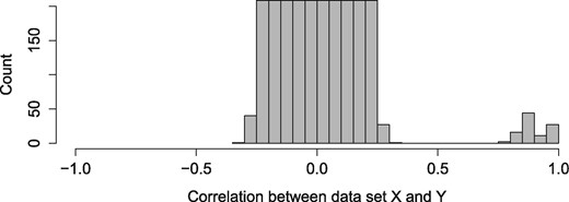
Histogram of the correlation between X and Y datasets. The associated variables have correlations of 0.9 with a standard deviation of 0.05, while the ‘noise’ variables are uniformly distributed between correlation of -0.4 and 0.4 (The histogram is pruned at Count = 200 for better visibility)

Fig. 3.

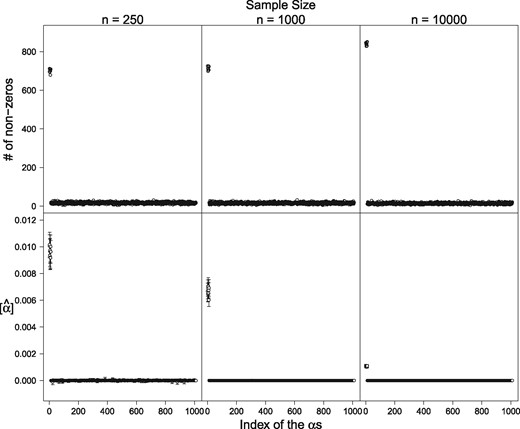
Results of the simulation studies. The upper row shows the total number of non-zero alphas over 1000 simulations, and the lower row shows the obtained mean alpha values with their 95% confidence interval

1. $\mathit{\xi }\in {\mathbb{R}}^n$ distributed $\mathbf{N}(0,1)$

2. $\mathit{X}\in {\mathbb{R}}^{n\times p}$

3. For $i=1,\dots ,w$⁠:

   • $\mathit{\alpha }\in {\mathbb{R}}^w$ distributed $\mathbf{N}(0.9,0.05)$$\wedge \hspace{0.17em}\mathit{\alpha }<1$

   • $x_i\in {\mathbb{R}}^n$ distributed $N({\alpha }_i\xi ,\sqrt{1-{\alpha }_i^2})$

4. For $i=1,\dots ,(p-w)$⁠:

   • $\mathit{\alpha }\in {\mathbb{R}}^{p-w}$ distributed $\mathbf{u}\mathbf{n}\mathbf{i}\mathbf{f}\left\{-0.4,0.4\right\}$

   • $x_{w+i}\in {\mathbb{R}}^n$ distributed $N({\alpha }_i\xi ,\sqrt{1-{\alpha }_i^2})$

5. $\mathit{X}={[x_1,\dots ,x_n]}^{\prime }$

The response dataset was created similarly.

The three scenarios differed in the number of rows the datasets contained. In the first scenario, both datasets X and Y contained 100 rows (n = 100, small sample size). We designed our second scenario similarly, but we increased the number of rows in both datasets X and Y from 100 to 250 (n = 250, medium sample size). In the third scenario, the number of rows was increased to 10 000 in both datasets (n = 10 000, large saFmple size).

We assessed the ability of the sRDA algorithm of identifying associated variables through measuring sensitivity and specificity. As we have set the w associated variables to the first w places among all p variables in the explanatory dataset, we defined specificity and sensitivity as follows; sensitivity (⁠$Sen{s}_1$⁠) is the measure of the number of variables assigned with non-zero regression weights at the first w positions in the explanatory dataset, divided by w;

$$\mathit{Sen}{s}_1=\frac{{\sum }_{i=1}^{w}I({\alpha }_i\ne 0)}{w}.$$

(8)

Additionally we have defined a second measure for sensitivity (⁠$Sen{s}_2$⁠) too, where we counted how many of the variables with the highest correlation weights are in the first w positions, and divided this number by w (thus this measure was not affected by the LASSO parameter since we only looked if the first w variables are among those having the highest correlation weights from all p variables).

Specificity (Spec) is defined as the measure of the number of variables assigned with zero regression weights among the variables at the last p-w positions in the explanatory dataset, divided by p-w;

$$\mathrm{Spec}=\frac{{\sum }_{i=w}^{p}I({\alpha }_i=0)}{p-w}.$$

(9)

We also report false discovery rate (FDR), defined by the proportion of not-associated variables assigned with a non-zero regression weights divided by all the number of all variables with a non-zero regression weight.

Both $Sen{s}_1$ and $Sen{s}_2$ measures resulted in high values (Table 1). $Sen{s}_1$ measures resulted between 0.70 and 0.83, $Sen{s}_2$ between 0.86 and 0.99, and FDR between 0.43 and 0.32 across the simulations. $Sen{s}_1$ and $Sen{s}_2$ are increased while FDR decreased in relation with increasing n. We measured a very high value for $Spec$⁠, 0.98, which was not much affected by the change of the sample size over the three simulations.

Table 1.

Simulation study results with multiple latent variables

	Sens1	Sens2	Spec	FDR
Small sample size	0.701	0.863	0.983	0.429
Medium sample size	0.714	0.948	0.984	0.352
Large sample size	0.839	0.992	0.986	0.318

4.1.2 Multiple latent variables

In the second simulation study, our objective was to assess the ability of sRDA of identifying multiple latent variables that are associated with the explanatory and response dataset, by assigning non zero regression weights to the associated variables.

4.1.2.1 Scenario of three latent variables

Similarly to the first simulation study’s settings, we generated two datasets. For the explanatory dataset, we generated 1000 variables that are not associated with the latent variables (⁠${\alpha }^{noise}\sim unif\left\{-0.4,0.4\right\}$⁠). Additionally, we added m variables in total, distributed in 3 groups (g = 3), with ${\mathit{\alpha }}^{assocd}$ coefficients that were associated with the latent variables which were sampled from the normal distribution with mean $\mu$ and standard deviation $\sigma$⁠;***** $m_1=10\hspace{0.17em}{\mathit{\alpha }}^{assocd}\hspace{0.17em}\sim \hspace{0.17em}\mathbf{N}(0.8,0.05)$⁠, $m_2=5\hspace{0.17em}{\mathit{\alpha }}^{assocd}\hspace{0.17em}\sim \hspace{0.17em}\mathbf{N}(0.7,0.05)$⁠, and $m_3=5\hspace{0.17em}{\mathit{\alpha }}^{assocd}\hspace{0.17em}\sim \hspace{0.17em}\mathbf{N}(0.6,0.05)$ (Fig. 4). These associated variables were placed at the first m positions among all variables (p). The response dataset was created similarly and both datasets had 1000 rows.

Fig. 4.

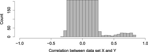
Histogram of the correlation between X and Y datasets. There are three groups of associated variables with correlations of 0.8, 0.7 and 0.6, with a standard deviation of 0.05. The ‘noise’ variables are uniformly distributed between correlation of −0.3 and 0.3

4.1.2.2 Scenario of five latent variables

We have created a similar scenario with 1000 variables that are not associated with the latent variables of the explanatory set (⁠${\mathit{\alpha }}^{noise}$ ∼ unif$\left\{-0.3,0.3\right\}$⁠), and we added five latent variable groups (g = 5), in total m variables; $m_1=5$${\mathit{\alpha }}^{assocd}$ ∼ $\mathbf{N}(0.5,0.05)$⁠, $m_2=5$${\mathit{\alpha }}^{assocd}$ ∼ $\mathbf{N}(0.7,0.05)$⁠, $m_3=10$${\mathit{\alpha }}^{assocd}$ ∼ $\mathbf{N}(0.8,0.05)$⁠, $m_4=10$${\mathit{\alpha }}^{assocd}$ ∼ $\mathbf{N}(0.6,0.05)$⁠, and $m_5=10$${\mathit{\alpha }}^{assocd}$ ∼ $\mathbf{N}(0.9,0.05)$⁠. Again, the associated variables were placed at the first m positions among all variables. The response dataset was created similarly and both datasets had 1000 rows.

4.1.2.3 Scenario of five latent variables—Univariate Soft Thresholding

We created a third scenario which is identical to the one above. Since it is shown that UST is much faster compared to ENet when the numbers of variables are large (Zou and Hastie, 2005), in this third scenario we applied UST penalization instead of the ENet.

To assess sRDA’s precision in latent variable detection, we defined the following sensitivity measure: the number of regression weight vectors from the first g returned regression weight vectors (regression weights for the latent variables, where g denotes the total number of associated variable groups) that had non zero regression weights (⁠$\mathit{\alpha }$⁠) among their first m variables (where m denotes the total number of variables of all the associated variable groups), divided by g.

We ran the simulations 1000 times in each case, with fixed values for the Ridge and LASSO penalties, 1 and 10, respectively (except for the five latent variables scenario, where the Ridge parameter is set to $\infty$ due to UST). The sensitivity scores presented are the average scores over the 1000 simulations (Table 2). We obtained a very high sensitivity score for both the 3 and 5 latent variables scenario, 0.996 and 0.987, respectively. Changing the penalization technique from ENet to UST dropped the sensitivity from 0.987 to 0.917.

Table 2.

Simulation study results with multiple latent variables

	Penalization method	Sensitivity
Three latent variables	Elastic net	0.996
Five latent variables	Elastic net	0.987
Five latent variables	Univariate soft thresholding	0.917

Assessing the computational time, on average it took 55.22 s to finish one simulation with the five latent variable scenario using ENet, while it took 11.65 seconds to conduct one simulation with the same settings, using UST.

4.2 Analysis of methylation markers and gene expression datasets

In our real data analysis scenario, our aim was to explain the variability in genomewide transciptomics data (i.e. gene expression) by genomewide epigenomic data (i.e. methylation markers). The datasets included data from 55 patients with Marfan Syndrome that participated in the Dutch Compare Trial (Groenink et al., 2013). The methylation markers from blood leukocytes are measured with the Illumina 450,000 technology, and the gene expression data are derived from skin biopsy using using Affymetrix Human Exon 1.0 ST Arrays (Radonic et al., 2012). The methylation markers (i.e. explanatory dataset) and the gene expression (i.e. response dataset) data contained 485 512 and 18 424 variables, respectively.

First we analysed these datasets using ENet for sRDA. The CV study was run in parallel on SURFSara’s Lisa Cluster (part of the Dutch national computer cluster; www.surfsara.nl) using 16 nodes and it took about 2.5 days.

Given the size of the data, we choose to use UST over the ENet version of our sRDA. We ran a 10-fold CV study to identify the optimal LASSO parameter, which resulted in 40 non-zero regression weights based on the highest sum of absolute correlations of $\mathit{\xi }$ and Y value of 8341.3 (O = 104.6, CI 95% = [18.3, 332.7]) Figure 5. The CV study and the analyses with the optimal LASSO parameter took 8059 and 189 seconds, respectively. The results are represented on Figure 6. Table 3 shows the correlations coefficients of the associated genes (i.e. those with the 10 highest correlation coefficients) in the first two latent variables.

Table 3.

The associated genes in the first two latent variables with their correlation coefficients

First latent variable		Second latent variable
Gene name	Correlation coefficient	Gene name	Correlation coefficient
ARPC3	0.8093	BCAS3	0.5902
C3orf23	0.8093	CADM1	0.6039
EXOC6	0.8008	CDKL5	0.6273
FAM118B	0.8155	GPC3	0.6025
GTPBP8	0.8178	ING4	0.5977
HSPH1	0.8073	LRIG3	0.6026
KIAA1841	0.8029	MGEA5	0.5947
KPNA2	0.8127	NONO	0.5970
RCH1	0.8048	SARNP	0.6047
RPS6KA3	0.8054	SUPV3L1	0.6014

Fig. 5.

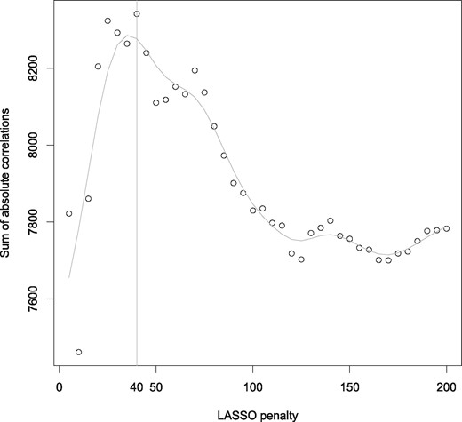
Optimal parameter selection for the LASSO parameter based on the sum of absolute correlations of $\mathit{\xi }$ and Y, using UST for sRDA

Fig. 6.

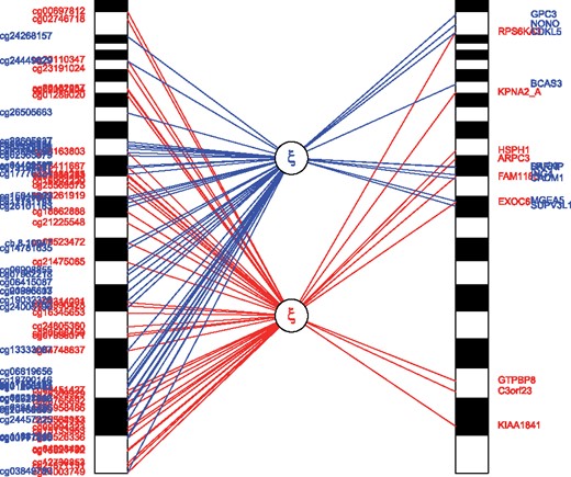
Representation of explaining the variability in genomewide transcriptomics data by genomewide epigenomic data using sRDA. The first (red, i.e. below) and the second (blue, i.e. upper) latent variable are shown. Relative to their genomic position, the methylation site names are placed on the left and the top 10 highly correlated associated genes are illustrated on the right (Color version of this figure is available at Bioinformatics online.)

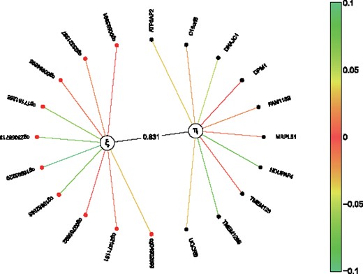
We used an over-representation analysis tool to link the highly associated genes (the top 10 with highest correlation coefficients) from the analysis of existing pathways. Multiple pathways were associated with the analysed genes from the first latent variable. The identified pathways included the ‘Cellular responses to stress’ (P 2.88 × 10⁻²), the ‘Regulation of HSF1-mediated heat shock response’ pathway (P 9.09 × 10⁻³) and the ‘Senescence-Associated Secretory Phenotype (SASP)’ pathway (P 7.5 × 10⁻²) (Fig. 6).

When analyzing the 10 genes with the highest correlation coefficients from the second latent variable, the identified pathways included the ‘Negative regulators of RIG-I/MDA5 signaling’ pathway (P 8.82$\times {10}^{-3}$⁠), the Diseases associated with glycosaminoglycan metabolism pathway (P 3.37 × 10⁻²) and the Nectin/Necl trans heterodimerization pathway (P 1.66 × 10⁻²) (Fig. 6).

We analysed the same datasets using sCCA in order to assess the required computational time. We used UST penalization method with a fixed LASSO parameter at 10. In the case of sCCA, this means that there were all but 10 variables’ regression weights set to zero from both datasets (Fig. 7). A single sCCA analysis on the same datasets took 575 s, while using sRDA took 267 s. After performing the permutation study 100 times, we observed that the sum of absolute correlation between $\mathit{\xi }$ and Y determined with the optimal LASSO parameter is not significantly different from the null distribution of the sum of absolute correlations (between $\mathit{\xi }$ and Y) of the real data.

Fig. 7.

Results of the sCCA analysis of the methylation markers and gene expressions dataset. Since sCCA searches for linear combinations from both datasets that results in the highest correlation between those linear combination (⁠$\mathit{\xi }$ and $\mathit{\eta }$⁠), and involves only multivariate regression, the regression weights are not interpretable as proportions of the total explained variance

5 Discussion

We proposed sparse Redundancy Analysis (sRDA) for high dimensional genetic and genomic data analysis as an alternative to sCCA. While sCCA is a symmetric multivariate statistical analysis, meaning that it does not make the distinction between the explanatory and predicted datasets, sRDA takes advantage on the prior knowledge of directionality that is often presumed by omics datasets. We showed that, compared to sCCA, sRDA performs better in terms of computational time and provides more easily interpretable results when the primary interest is to explain the variance in the particular predicted variables (e.g. genes in gene expression data) from the linear combination of predictive variables (e.g. from the combined effect of methylation sites).

Our simulation study shows that the implementation of our sRDA algorithm can identify multiple latent variables that are associated with the explanatory and response dataset, with high sensitivity and specificity measures. Our software implementation is compliant with parallel computing and therefore computational time can be further reduced. We implemented different penalization methods (Ridge, LASSO, UST) to further optimize our analysis procedure and showed scenarios where applying different penalization methods can lead to a five times faster computational time without a serious decrease of the algorithms ability to identify highly correlated variables (it took 55.22 s to analyse five latent variable using ENet (with sens = 0.987), while using UST took 11.65 s (with sens = 0.917) for the same data).

Through the analysis of 485 512 methylation markers and 18,424 gene-expression values measured in a subset of 55 patients with Marfan syndrome, we showed that sRDA is able to deal with the usual high dimensionality of omics data and performs better optimized compared to sCCA (267 and 575 seconds, respectively). Through permutation study, we observed that the optimal criterion value we obtained during the real data scenario is not significantly different from the values we obtained during the permutation study. We assume that this is due to the low sample size of our data (n = 55).

Although Takane and Hwang (2007) introduced a theoretical framework for regularized redundancy analysis in order to deal with the problem of multicollinearity in the explanatory variables, their framework relies on the Ridge penalization technique thus it only shrinks the regression coefficients towards zero but does not set them to zero, which makes interpretation of results difficult if there are thousands or even millions of variables. One important strength of our proposed method is the ability to set regression coefficients to zero. Since sRDA uses a univariate regression step to derive the weights for the response variables, the regression weights for the response variables can be interpreted as the variance of each individual variable proportionally contributed to the total variance we explain in the response dataset from the explanatory dataset. Thus in our real data scenario, we can interpret the regression weights (⁠$\mathit{\beta }$⁠) (i.e. the regression coefficients of the gene expression dataset) as each gene’s individual contribution to the total variance that the linear combination of variables in the methylation marker dataset explains in the gene expression dataset (Table 3), and the sum of the correlation between Y and $\mathit{\xi }$ is equal to the sum of these regression weights (⁠$\mathit{\beta }$⁠), since in our case $\mathit{\beta }$ is the correlation coefficient. Thus the regression weights of the response variables provide easily interpretable results (e.g., 10 genes can be selected from the gene expression dataset that have the highest correlation coefficient with the linear combinations of the corresponding methylation markers, as illustrated in Fig. 6). This property does not hold for sCCA (Fig. 7). Therefore, sRDA both improves on the interpretability of results and on the computational time compared to sCCA.

6 Conclusion

Integromics research aims to explain genotype-phenotype relations in patients and uses mainly high dimensional omics data to accomplish that. Recently there has been much interest in associating multiple phenotypes with multiple genetic and or genomic datasets. Current implementations of multivariate statistical methods either cannot deal with the high dimensionality of genetic and genomic datasets or perform suboptimally. We proposed sparse Redundancy Analysis (sRDA) for high dimensional genetic and genomic data analysis. We built a software implemented of our algorithm and conducted simulation studies on SURFsara’s Lisa computer cluster to assess the reliability of sRDA. Analysis of 485 512 methylation markers and 18 424 gene-expression values measured in a subset of 55 patients with Marfan syndrome shows that sRDA is able to deal with the usual high dimensionality of omics data and performs better optimized compared to sCCA. Our sRDA’s algorithm is easily extendable to analyse multiple omics sets. Such an generalized version of sRDA could become an optimal statistical method for multiple omics sets analysis.

Conflict of Interest: none declared.