


Abstract
Mining relations between chemicals and proteins from the biomedical literature is an increasingly important task. The CHEMPROT track at BioCreative VI aims to promote the development and evaluation of systems that can automatically detect the chemical–protein relations in running text (PubMed abstracts). This work describes our CHEMPROT track entry, which is an ensemble of three systems, including a support vector machine, a convolutional neural network, and a recurrent neural network. Their output is combined using majority voting or stacking for final predictions. Our CHEMPROT system obtained 0.7266 in precision and 0.5735 in recall for an F-score of 0.6410 during the challenge, demonstrating the effectiveness of machine learning-based approaches for automatic relation extraction from biomedical literature and achieving the highest performance in the task during the 2017 challenge.
Database URL: http://www.biocreative.org/tasks/biocreative-vi/track-5/
Introduction
Recognizing the relations between chemicals and proteins is crucial in various tasks such as precision medicine, drug discovery and basic biomedical research. Biomedical researchers study various associations between chemicals and proteins and disseminate their findings in scientific publications. Although manually extracting chemical–protein relations from the biomedical literature is possible, it is costly and time-consuming. Alternatively, text-mining methods could automatically detect these relations effectively. The BioCreative VI track 5 CHEMPROT task (http://www.biocreative.org/tasks/biocreative-vi/track-5/) aims to promote the development and evaluation of systems that can automatically detect and classify relations between chemical compounds/drug and proteins (1) in running text (PubMed abstracts).
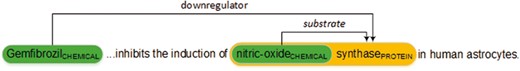
Figure 1 shows an example of chemical–protein annotations in PMID 12244038. The relation encoded in the text is represented in a standoff-style annotation as follows. Note that, the organizers used ‘gene’ and ‘protein’ interchangeably in this task.
| 1 | 12244038 | T17 | CHEMICAL | 0 | 11 | Gemfibrozil |
| 2 | 12244038 | T18 | CHEMICAL | 62 | 74 | nitric-oxide |
| 3 | 12244038 | T68 | GENE-N | 62 | 83 | nitric-oxide synthase |
| 4 | 12244038 | CPR: 4 | Arg1: T17 | Arg2: T68 | ||
| 5 | 12244038 | CPR: 9 | Arg1: T18 | Arg2: T68 | ||
| 1 | 12244038 | T17 | CHEMICAL | 0 | 11 | Gemfibrozil |
| 2 | 12244038 | T18 | CHEMICAL | 62 | 74 | nitric-oxide |
| 3 | 12244038 | T68 | GENE-N | 62 | 83 | nitric-oxide synthase |
| 4 | 12244038 | CPR: 4 | Arg1: T17 | Arg2: T68 | ||
| 5 | 12244038 | CPR: 9 | Arg1: T18 | Arg2: T68 | ||
| 1 | 12244038 | T17 | CHEMICAL | 0 | 11 | Gemfibrozil |
| 2 | 12244038 | T18 | CHEMICAL | 62 | 74 | nitric-oxide |
| 3 | 12244038 | T68 | GENE-N | 62 | 83 | nitric-oxide synthase |
| 4 | 12244038 | CPR: 4 | Arg1: T17 | Arg2: T68 | ||
| 5 | 12244038 | CPR: 9 | Arg1: T18 | Arg2: T68 | ||
| 1 | 12244038 | T17 | CHEMICAL | 0 | 11 | Gemfibrozil |
| 2 | 12244038 | T18 | CHEMICAL | 62 | 74 | nitric-oxide |
| 3 | 12244038 | T68 | GENE-N | 62 | 83 | nitric-oxide synthase |
| 4 | 12244038 | CPR: 4 | Arg1: T17 | Arg2: T68 | ||
| 5 | 12244038 | CPR: 9 | Arg1: T18 | Arg2: T68 | ||
Chemical–protein annotation example.
The annotation T17 identifies a chemical, ‘Gemfibrozil’, referred by the string between the character offsets 0 and 11. T18 identifies another chemical, ‘nitric-oxide’ and T68 identifies a protein, ‘nitric-oxide synthase’. Line 4 then represents the chemical–protein relation with type ‘downregulator’ (CPR: 4) and the arguments T17 and T68. Line 5 represents a ‘substrate’ (CPR: 9) relation with arguments T18 and T68. Note that T18 is enclosed in T68 in this example which is allowable in the task.
The goal of the CHEMPROT task is to find the full representation as in Lines 4 and 5. From the machine-learning perspective, we formulate the CHEMPROT task as a multiclass classification problem where discriminative classifiers are trained with a set of positive and negative relation instances. Although various discriminative methods have been studied, in the last decade, support vector machines (SVMs) with a set of features or rich structural representations like trees or graphs have achieved the state-of-the-art performance (2, 3).
Deep neural networks have recently achieved promising results in the biomedical relation extraction task (4). When compared with traditional machine-learning methods, they may be able to overcome the feature sparsity and engineering problems. For example, various convolutional neural networks (CNNs) were found to be well-suited for protein–protein interaction and chemical-induced disease extraction (5–7). Furthermore, recurrent neural networks (RNNs) with multiple attention layers have been used to extract drug–drug interactions from text (8, 9). For the CHEMPROT task in BioCreative VI, we observed both CNNs and RNNs were widely used (10–16).
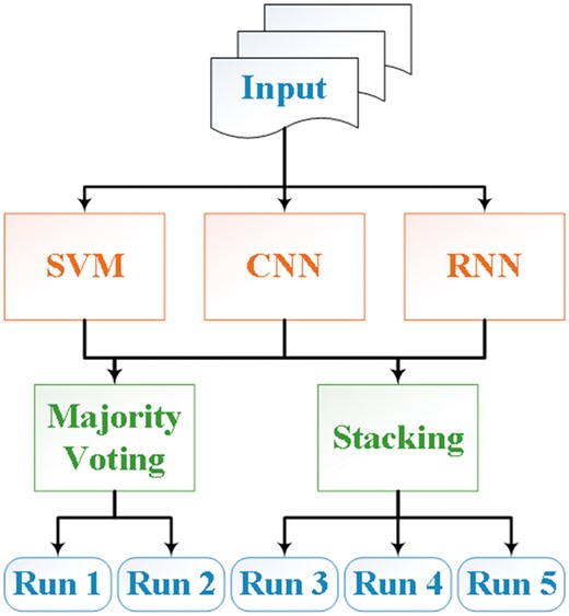
In this article, we describe our approaches and results for the CHEMPROT task at BioCreative VI. The contribution of our project is to propose an ensemble of three state-of-the-art systems: SVMs, CNNs and RNNs. The outputs of the three systems are combined using either majority voting or stacking.
During the CHEMPROT 2017 shared task, the organizers released human-annotated training and development sets, but not the test set. Based on the released dataset, first we trained three individual systems using 80% of the combination of training and development datasets. Then we used the remaining 20% for choosing the ensemble methods. Experiments on the official test set show that we obtained the best performance in F-score. After the challenge, we conducted further analysis on different characteristics of positive pairs such as the sentence length and the entity distance. Our observation indicated that pairs are more difficult to classify in longer sentences and the RNN model can detect distant pairs better than other individual models.
Materials and methods
Dataset
In the CHEMPROT track, the organizers developed a chemical–protein relation corpus composed of 2432 PubMed abstracts, which were divided into a training set (1020 abstracts), development set (612 abstracts) and test set (800 abstracts) (1). Table 1 shows the dataset statistics.
Statistics of the CHEMPROT dataset
| Training | Development | Test | |
|---|---|---|---|
| Document | 1020 | 612 | 800 |
| Chemical | 13017 | 8004 | 10810 |
| Protein | 12752 | 7567 | 10019 |
| Positive relation | 4157 | 2416 | 3458 |
| CPR: 3 | 768 | 550 | 665 |
| CPR: 4 | 2254 | 1094 | 1661 |
| CPR: 5 | 173 | 116 | 195 |
| CPR: 6 | 235 | 199 | 293 |
| CPR: 9 | 727 | 457 | 644 |
| Positive relation in one sentence | 4122 | 2412 | 3444 |
In the dataset, both chemical and protein mentions were pre-annotated, and there are five types of chemical–protein relations, the biological properties upregulator (CPR: 3), downregulator (CPR: 4), agonist (CPR: 5), antagonist (CPR: 6) and substrate (CPR: 9). Hence, given all chemical–protein pairs as candidates, the goal of this task is to predict whether the pair is related or not. Also, if the chemical–protein pair is related, then we must predict the relation type.
Unlike other relation corpora (17, 18), cross-sentence relations are rare in this corpus, appearing in <1% of the training set. We also noticed that some chemical–protein pairs have multiple labels, but they only appear less than ten times in the training set. As a result, our system treated the relation extraction task as a multiclass classification problem, and to simplify the problem, our system only focused on the chemical–protein relations occurring in a single sentence.
Methods
During the shared task, we hypothesized that an ensemble system that combines results of different methods could lead to better predictive performance than using a single method (19, 20). Hence, we addressed the CHEMPROT task using two ensemble systems that combined the results from three individual models, similar to our previous BioCreative submissions (21). An overview of the system architecture is shown in Figure 2. The individual systems included are an SVM, a CNN and an RNN (2, 22, 23). We will describe these models together with the ensemble algorithms in the following subsections.
Architecture of the systems for the CHEMPROT task.
Feature rich SVM
An SVM is a discriminative classifier formally defined by a separating hyperplane that uses hinge loss (2). Given a set of training examples, linear SVMs find the hyperplane that separates positives and negatives with a maximum margin. If the two sets are not linearly separable, the SVM uses the kernel trick to implicitly map inputs into high-dimensional feature spaces where the examples might be separable. In our SVM system, the following features are exploited.
Words surrounding the chemical and protein mentions of interest: These features include the lemma form of a word, its part-of-speech tag, and chunk types. We used the Genia Tagger to extract the features (24). We set the window size to five.
Bag-of-words between the chemical and protein mentions of interest in a sentence: These features include the lemma form of a word and its relative position to the target pair of entities (before, middle and after).
The distance (the number of words) between two entity mentions in a sentence.
The existence of a keyword between two mentions often implies a specific type of a relation, such as ‘inhibit’ for relation ‘CPR: 4’ and ‘agonism’ for relation ‘CPR: 5’. Therefore, we manually built the keyword list from the training set and used them as features as well.
Shortest-path features include vertex walks (v-walks) and edge walks (e-walks) between the target entities in a dependency parse graph (25). An e-walk includes constituents with each word and its two dependencies. Each v-walk’s constituents include two words and the connecting dependency relation. For example, the shortest path of <Gemfibrozil, nitric-oxide synthase> extracted from the sentence ‘GemfibrozilCHEMICAL, a lipid-lowering drug, inhibits the induction of nitric-oxide synthasePROTEIN in human astrocytes.’ is ‘Gemfibrozil ← nsubj ← inhibits → dobj → induction → nmod: of → nitric-oxide synthase’. Thus the e-walks are ‘nsubj—inhibits—dobj’ and ‘dobj – induction – nmod: of’. The v-walks are ‘Gemfibrozil – nsubj – inhibits’, ‘inhibits – dobj – induction’ and ‘induction – nmod: of – nitrix-oxide synthase’.
We trained the SVM system using a linear kernel (http://scikit-learn.org/). In our submissions, we set the penalty parameter C to 1 and the tolerance for stopping criteria to 1e-3. We also balanced the feature instances by adjusting their weights inversely proportional to class frequencies in the training set and used the one-vs-rest multiclass strategy.
Convolutional neural networks
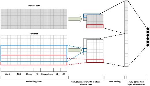
We followed the work of Peng and Lu (5) to build our CNN model. Instead of using multichannels, we applied one channel but used two input layers (Figure 3). One is the sentence sequence and the other is the shortest path between the pair of entity mentions in the target relation. For example, we use two inputs of the above example in the CNN: the original sentence ‘Gemfibrozil, a lipid-lowering drug, inhibits the induction of nitric-oxide synthase in human astrocytes’ and the shortest path ‘Gemfibrozil inhibits induction nitric-oxide synthase’.
Overview of the CNN model.
In our model, we represent each word (in either a sentence or a shortest path) by concatenating embeddings of its words, part-of-speech tags, chunks, named entities, dependencies and positions relative to the two mentions of interest. We learned the pre-trained word embedding vectors on PubMed articles using the gensim word2vec implementation with the dimensionality set to 300 (26). We obtained the part-of-speech tags, chunks and named entities from the Genia Tagger (24).
We extracted the dependency information using the Bllip parser with the biomedical model and the Stanford dependencies converter (27–29). For each word, we used the dependency label of the “incoming” edge of that word in the dependency graph. We encoded the dependency features using a one-hot scheme, and their dimensionality is 101.
For each input layer, we applied convolution to inputs to get local features with window sizes of 3 and 5. For each convolution, we subsequently applied the rectified linear unit activation function and performed 1–max pooling to get the most useful global feature from the entire sentence. In the fully connected layer, we concatenated the global features from both the sentence and the shortest path and then applied a fully connected layer to the feature vectors and a final softmax to classify the six classes (five positive + one negative). We also used the dropout of 0.5 to prevent overfitting.
We trained all parameters using the Adam algorithm to optimize the cross-entropy loss on a mini-batch with a batch size of 32 (30). We updated the embeddings (word, part-of-speech, chunk, position, dependency and distance) during training.
Recurrent neural networks
For our RNN model, we built on the work of Kavuluru et al. (9). Specifically, we trained a bi-directional long-short term-memory (Bi-LSTM) recurrent model (Figure 4), where the input to the model is a sentence (hence the corresponding word embeddings).
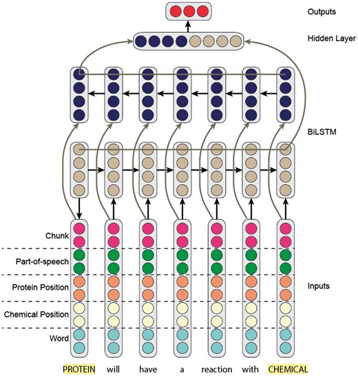
Overview of the RNN model.
Like our CNN model, we concatenated the word embedding with the part-of-speech, IOB-chunk tag and two position embeddings. The two position embeddings represent the relative location of the word with respect to the two entity mentions. It is important to note that we updated the embeddings (word, part-of-speech, chunk and position) during training.
After passing a sentence through our Bi-LSTM model, we obtained two hidden representations for each word—one representing the forward context and the other representing the backward. We concatenated the two representations to obtain the final representation of each word. To obtain a representation of the sentence, we used max-over-time (1–max) pooling across hidden state word representations.
Next, we passed the max-pooled sentence representation to a fully connected output layer. Unlike our CNN, we only applied a linear transformation without a softmax operation. Furthermore, the output layer only had five classes, where we completely discarded the negative class. Specifically, we used the pairwise ranking loss proposed by (31). Intuitively, the negative class would be noisy compared with the five positive classes. Rather than learning to predict the negative class explicitly, we forced the five outputs to be negative. At prediction time, if all positive class scores were negative, we predicted the negative class. Otherwise, we predicted the class with the largest positive score.
Before training our model, we preprocessed the dataset by replacing each word in the corpus that occurs less than five times with an unknown (UNK) token. Also, given each instance was comprised of a sentence and two entity mentions, we replaced each entity with the tokens CHEMICAL or PROTEIN dependent on what the specific mention represented.
Finally, we trained our RNN model using the Adam optimizer with a mini-batch size of 32. For the Adam optimizer, we set the learning rate to 0.001, beta1 to 0.9 and beta2 to 0.999. In addition, we applied recurrent dropout of 0.2 in the Bi-LSTM model and standard dropout of 0.2 between the max-pooling and output layers. We used pre-trained word vectors (6B Token GLOVE (https://nlp.stanford.edu/projects/glove/)) with a dimensionality of 300. Likewise, the POS, position, and chunk vectors were randomly initialized, and each had a dimensionality of 32. We should note that both the POS and chunk tags were extracted using NLTK (http://www.nltk.org/). Last, we set the hidden state size of the LSTM models to 2048.
A majority voting system
In our first ensemble system, we combined the results of the three models using majority voting. That is, we selected the relations that were predicted by >2 models. If we could not get a majority vote on a relation instance (e.g. SVM predicted CPR: 3, CNN CPR: 4 and RNN CPR: 5), we predicted the ‘negative’ class for this instance.
A stacking system
In our second system, we used the stacking method to combine the predictions of each model. Stacking works by training multiple base models (SVM, CNN and RNN), then trains a meta-model using the base model predictions as features.
For our meta-model, we trained a random forest (RF) classifier (http://scikit-learn.org). First, to train the RF, we computed the scores for each class from all three models on the development set. In total, we had the following 17 features: 6 from the SVM, 6 from CNN and 5 from the RNN (because we used a ranking loss). For the CNN scores, we used the unnormalized scores for each class before passing them through the softmax function. Finally, we trained the RF on the development set using 50000 trees and the gini splitting criteria.
Results
We prepared our submissions with an ensemble of three models. The training and development sets (a total of 1632 articles) were made available to participating teams during their system development and validation phase. As shown in Figure 5, we built every SVM, CNN and RNN model using 60% total data, built the ensemble system using the 20% and tested the systems using the remaining 20%. Table 2 shows the cross-validation performance of our systems, where ‘P’, ‘R’ and ‘F’ denotes precision, recall and F1 score, respectively.
Results for our individual and ensemble systems with training and development sets
| System | P | R | F |
|---|---|---|---|
| SVM | 0.6291 | 0.4779 | 0.5430 |
| CNN | 0.6406 | 0.5713 | 0.6023 |
| RNN | 0.6080 | 0.6139 | 0.6094 |
| Majority voting | 0.7408 | 0.5517 | 0.6319 |
| Stacking | 0.7554 | 0.5524 | 0.6378 |
| System | P | R | F |
|---|---|---|---|
| SVM | 0.6291 | 0.4779 | 0.5430 |
| CNN | 0.6406 | 0.5713 | 0.6023 |
| RNN | 0.6080 | 0.6139 | 0.6094 |
| Majority voting | 0.7408 | 0.5517 | 0.6319 |
| Stacking | 0.7554 | 0.5524 | 0.6378 |
Macro-average results are reported using 5-fold cross validation.
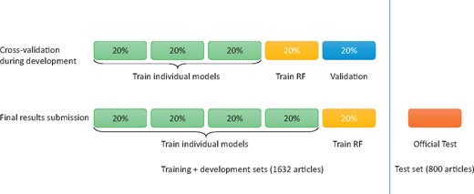
Data partition of 5-fold cross-validation and final submission.
For our final submission, we built every SVM, CNN and RNN model using 80% total data in the training and development sets and built the ensemble system using the remaining 20% of the total data. To reduce variability, we performed 5-fold cross-validation using different partitions of the data. As a result, we obtained five SVMs, five CNNs and five RNNs in total. Table 2 shows the cross-validation performance of our systems, where ‘P’, ‘R’ and ‘F’ denotes precision, recall and F1 score, respectively. Table 3 shows the overall performance of our systems on the official test set, where ‘TP’, ‘FP’ and ‘FN’ denotes true positive, false positive and false negative, respectively.
Results for our ensemble systems on test set
| System | Fold | TP | FP | FN | P | R | F |
|---|---|---|---|---|---|---|---|
| SVM | 1 | 1646 | 875 | 1812 | 0.6529 | 0.4760 | 0.5506 |
| 2 | 1654 | 1001 | 1804 | 0.6230 | 0.4783 | 0.5411 | |
| 3 | 1668 | 932 | 1790 | 0.6415 | 0.4824 | 0.5507 | |
| 4 | 1679 | 911 | 1779 | 0.6483 | 0.4855 | 0.5552 | |
| 5 | 1646 | 963 | 1812 | 0.6309 | 0.4760 | 0.5426 | |
| CNN | 1 | 2040 | 1280 | 1418 | 0.6145 | 0.5899 | 0.6019 |
| 2 | 1996 | 1075 | 1462 | 0.6500 | 0.5772 | 0.6114 | |
| 3 | 2031 | 1254 | 1427 | 0.6183 | 0.5873 | 0.6024 | |
| 4 | 1961 | 1073 | 1497 | 0.6463 | 0.5671 | 0.6041 | |
| 5 | 1970 | 1107 | 1488 | 0.6402 | 0.5697 | 0.6029 | |
| RNN | 1 | 2085 | 1333 | 1373 | 0.6100 | 0.6029 | 0.6065 |
| 2 | 2255 | 1601 | 1203 | 0.5848 | 0.6521 | 0.6166 | |
| 3 | 2112 | 1390 | 1346 | 0.6031 | 0.6108 | 0.6069 | |
| 4 | 2097 | 1316 | 1361 | 0.6144 | 0.6064 | 0.6104 | |
| 5 | 2322 | 1845 | 1136 | 0.5572 | 0.6715 | 0.6090 | |
| Majority voting | 1 | 1966 | 723 | 1492 | 0.7311 | 0.5685 | 0.6397 |
| 2 | 1983 | 746 | 1475 | 0.7266 | 0.5735 | 0.6410 | |
| 3 | 1962 | 715 | 1496 | 0.7329 | 0.5674 | 0.6396 | |
| 4 | 1934 | 697 | 1524 | 0.7351 | 0.5593 | 0.6352 | |
| 5 | 2020 | 784 | 1438 | 0.7204 | 0.5842 | 0.6452 | |
| Stacking | 1 | 1890 | 641 | 1568 | 0.7467 | 0.5466 | 0.6312 |
| 2 | 1756 | 530 | 1702 | 0.7682 | 0.5078 | 0.6114 | |
| 3 | 1912 | 659 | 1546 | 0.7437 | 0.5529 | 0.6343 | |
| 4 | 1903 | 710 | 1555 | 0.7283 | 0.5503 | 0.6269 | |
| 5 | 1861 | 645 | 1597 | 0.7426 | 0.5382 | 0.6241 |
Submitted runs are reported in bold text.
During the CHEMPROT task, we submitted five runs as our final submissions (bolded in Table 3). For each method we trained five models using different training/test splits (based on 5-fold CV). Each of our final submissions is based on the best method for each of the folds. For example, Submissions 1 and 2 use a majority voting system. These runs were chosen based on their respective folds performance on the validation dataset. Thus, voting was the best method on folds 1 and 2 and stacking was best for Folds 3–5 on each fold test split. Unfortunately, we found that stacking overfit on the training dataset, and voting performed best overall. Therefore, our best system was not submitted in the competition. Based on our submitted models, our CHEMPROT system obtained 0.7266 in precision and 0.5735 in recall for an F-score of 0.6410, achieving the highest performance in the task during the 2017 challenge. Our best method in Table 3 (Majority voting on Fold 5) achieved the overall best F-score of 0.6452.
Discussion
In the following subsections, we perform error analysis for each of our methods: SVM, CNN, RNN, voting and stacking. To easily compare each method, we only focus on models trained with the same dataset split, Fold 1. Overall, we analyze how different the predictions are among the methods. Detailed predictions are provided in the supplementary document. Next, we look at how the length of each sentence and the distance between entity pairs affects each model’s performance.
Analysis of difficult pairs
In this experiment, we aim to determine the difficulty of classifying chemical–protein pairs. We partitioned the positive chemical–protein relations into four groups based on the number of approaches (SVM, CNN and RNN) that correctly predict it. For example, if all the approaches correctly predicted a given relation, then the number of approaches that could correctly classify the relation is three. We hypothesize that the fewer number of approaches that can classify a pair correctly, the more difficult the pair. Figure 6 shows the distribution of pairs in the four groups. Among 3458 positive chemical–protein relations, 1792 pairs were detected by all three models (called easy pairs), whereas 492 pairs were not detected by any of the models (called difficult pairs). Here, we show that some pairs were inherently difficult to classify (across all approaches). In Table 4, we count the number of times each method correctly predicts relations in each group. Among the 481 relations that could be classified correctly by only one of the three basic methods (SVM, CNN and RNN), the SVM correctly predicted 30 relations (CNN: 120, RNN: 331) in that group. If no models could predict a pair, the majority voting method could not predict it either (Table 4, row 0, column Majority voting). If only one model could predict a pair, the majority voting method still cannot predict it, because it needs one pair being predicted by at least two models (Table 4, row 1, column Majority voting). On the other hand, we observed that the stacking method could select true positive pairs even if just one or even when none of the models could predict it (Table 4, row 0 and 1, column Stacking).
The distribution of pairs for each model according to the number of approaches that can correctly classify a given pair
| No. of approaches | SVM | CNN | RNN | Majority voting | Stacking |
|---|---|---|---|---|---|
| 0 | 0 | 0 | 0 | 0 | 3 |
| 1 | 30 | 120 | 331 | 0 | 91 |
| 2 | 187 | 565 | 634 | 602 | 534 |
| 3 | 1792 | 1792 | 1792 | 1790 | 1770 |
| No. of approaches | SVM | CNN | RNN | Majority voting | Stacking |
|---|---|---|---|---|---|
| 0 | 0 | 0 | 0 | 0 | 3 |
| 1 | 30 | 120 | 331 | 0 | 91 |
| 2 | 187 | 565 | 634 | 602 | 534 |
| 3 | 1792 | 1792 | 1792 | 1790 | 1770 |
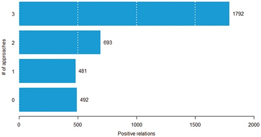
The distribution of pairs according to the number of approaches that can correctly classify a given pair.
Relation between sentence length, inter entity distance and pair difficulty
Figure 7 shows the characteristics of sentence difficulty in terms of the average length of the sentence and the average distance between entities. We observed that pairs were more difficult to classify in longer sentences. On the other hand, the distance between entities in a sentence seemed to not have much impact on performance.
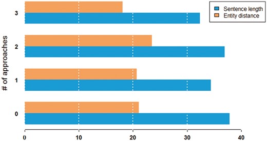
Average sentence length and entity distance in words by the number of approaches that can correctly classify a given pair.
Figures 8 and 9 show the relation between sentence length, inter entity distance and true positive instances predicted by individual models. Both figures suggest that the RNN model can detect distant pairs better than other models. Intuitively, CNN models learn to extract informative n-grams from text, while RNNs better model the sequential nature of each sentence.
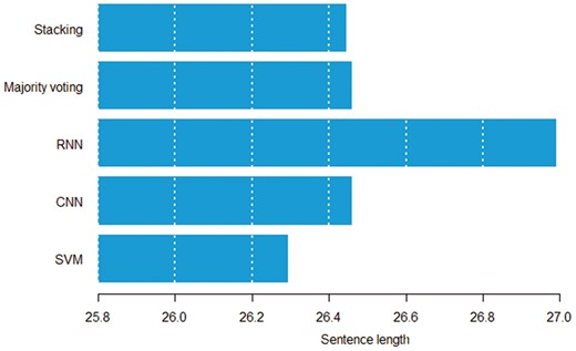
Average sentence length in words by the model that can correctly classify a given pair.
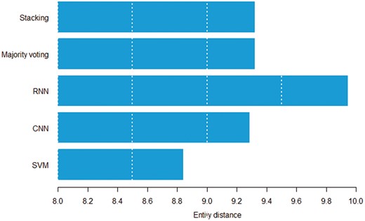
Average entity distance in words by the model that can correctly classify a given pair.
Conclusion
In this article, we described our submission in the BioCreative VI CHEMPROT task. The results demonstrate that our ensemble system can effectively detect the chemical–protein relations from biomedical literature. In addition, we analyzed the results of both individual and ensemble systems on the test set and demonstrate how well each model performs across various characteristics (sentence length and distance between entities) of positive chemical–protein pairs.
In the future, we would like to investigate if an external knowledge base can be used to improve our model, e.g. via attributes of chemicals and proteins from PubChem and the Protein Ontology. We are also interested in extending the method to chemical–protein relations that manifest beyond the sentence boundaries. Finally, we would like to test and generalize this approach to other biomedical relations such as protein–protein interactions (5).
Acknowledgements
The authors thank the organizers of the BioCreative VI CHEMPROT track for their initiative and efforts in organizing the task and releasing the datasets used in this article.
Funding
This work was supported by the Intramural Research Programs of the National Institutes of Health, National Library of Medicine [Y.P. and Z.L.] and through an extramural National Library of Medicine grant [R21LM012274 to A.R. and R.K.]. A.R. was a summer intern at the NCBI/NIH and supported by the NIH Intramural Research Training Award.
Conflict of interest. None declared.
References
Author notes
Citation details: Peng,Y., Rios,A., Kavuluru,R. et al. Extracting chemical–protein relations with ensembles of SVM and deep learning models. Database (2018) Vol. 2018: article ID bay073; doi:10.1093/database/bay073
