Utility, Risk and Demand for Incomplete Insurance: Lab Experiments with Guatemalan Co-Operatives

Abstract

We play a series of incentivised laboratory games with risk-exposed co-operativised Guatemalan coffee farmers to understand the demand for index-based rainfall insurance. We estimate an explicit utility curve for every player and hence predict expected utility demand under counterfactual scenarios. Using these estimates, we provide a precise money-metric decomposition of the extent to which the low observed demand for index insurance is driven by expected utility theory, or by behavioural issues arising from a prospect-style utility structure. Our results suggest that consumers value probabilistic insurance using a prospect-style utility function that is concave both in probabilities and in income.

Despite the central importance of risk preferences in economics and the potential for insurance to solve risk-driven poverty traps (Brick and Visser, 2015), our understanding of the drivers of insurance demand remains incomplete. The welfare benefits of insurance appear to be particularly important in agriculture, where weather risk plays a dominant role (Rosenzweig and Binswanger, 1992). New types of index insurance, in which payouts are based on a pre-defined index (such as local rainfall), can provide insurance against aggregate shocks without creating moral hazard (Barnett and Mahul, 2007). From a perspective motivated by the Townsend (1994) model of village-level risk pooling, these products appear ideal in that they insure precisely the correlated shock that cannot be smoothed by local risk-pooling mechanisms. Yet, when introduced in the field, these products have almost universally met with disappointing demand (Cole et al., 2013) and several studies have found that interlinking index insurance with credit products actually dampens the demand for credit (Giné and Yang, 2009; Banerjee et al., 2014). Low demand for these apparently welfare-improving insurance contracts is puzzling, and so a deeper understanding of consumer risk preferences is critical.

A well-established feature of index insurance products is the issue of ‘basis risk’, which arises because the index is only imperfectly correlated with the risk against which it is meant to protect (Barnett et al., 2008). Wrapped up in this omnibus term are a number of distinct components that may have very different effects on demand. Insurance may be imperfect because it is partial, meaning that payouts fail to cover the full value of losses. Imperfect insurance can also be probabilistic, meaning that there are important shocks that are imperfectly correlated with the index. While response to the former type of risk has typically been found to be easily modelled in an expected utility (EU) framework (Camerer, 2004; Cohen and Einav, 2007; Barseghyan et al., 2013), a large empirical literature has suggested a prominent role for behavioural drivers in depressing demand for probabilistic insurance (Kahneman and Tversky, 1979; Tversky and Kahneman, 1992; Wakker et al., 1997). In particular, numerous experimental studies have suggested that people overweight the likelihood of small probabilities, and thus have utility that is concave in probabilities (Yaari, 1987; Doherty and Eeckhoudt, 1995). Finally, demand is also likely to interact in complex ways with the nature of complementary institutions such as pre-existing informal risk pooling (Mobarak and Rosenzweig, 2014). Understanding the extent to which the workhorse expected utility model does or does not explain demand for these novel insurance products is a matter both of theoretical interest and of substantial policy importance.

In this article we construct a unique empirical environment that gives us a money-metric quantification of the extent to which insurance demand is driven by expected utility theory. We conducted a set of controlled lab-in-the-field games with a very risk-exposed group: co-operative-based smallholder coffee farmers in Guatemala. During the course of an incentivised day-long exercise, we presented farmers with a way of visualising the weather-driven risks to their farms and recorded their willingness to pay (WTP) for an excess rainfall index insurance product across multiple scenarios.¹ These tightly framed games provide a straightforward way of observing how individuals weigh different outcomes in decision making (Harrison and Ng, 2016).² Truthful revelation of the WTP was incentivised with a Becker-Degroot-Marschak mechanism, with the selection of one of the scenarios at the end of the day to determine the compensation that each participant received.

An initial set of scenarios measuring WTP for partial insurance is used to estimate a utility curve for every player. We can then use these utility curves to predict what WTP should be in alternate scenarios where the risk and payout structures are more complex. We utilise this tool to examine two central issues in insurance demand. First, how does demand for insurance respond when the risk environment is multi-peril? Second, how does demand respond when the product is provided in a manner intended to induce group risk pooling?

In the benchmark partial insurance game, we present seven scenarios that vary the severity and the variance of the loss in the insured states of nature. These scenarios effectively measure the marginal utility of income in a shock state as it becomes more severe, and therefore provide a straightforward window to the shape of the utility curve across states of nature. We confirm other studies in finding a low overall demand for index insurance; only 12% of our sample were willing to pay a price above the actuarially fair price in our base scenario. We use a non-linear least squares optimisation method to fit a two-parameter utility function for each player on his stated WTP across these seven scenarios. The estimated utility curves display an average coefficient of relative risk aversion of 5.8 and a modal utility function that has very close to constant absolute risk aversion. Once we have a direct model of utility curves, we can predict an ‘EU-based’ WTP for an insurance in any other risk scenario, assuming that the standard mechanics of concave utility are the only source of demand for insurance. This dollar-denominated estimate of EU WTP from the benchmark partial insurance game gives us a means to decompose the drivers of demand in alternate, more complex risk scenarios.

The first application of our estimated WTP is to the probabilistic insurance game, in which we presented a set of scenarios varying the severity and probability of a shock that occurs with no insurance payout. As predicted by a sizeable behavioural literature, this possibility of contract failure causes a substantial drop in WTP. When we decompose the demand into the component predicted by expected utility maximisation and the ‘behavioural’ residual, we find that the behavioural dampening in WTP responds strongly both to the probability and the magnitude of the uninsured shock. Adding a 1 in 21 chance of a small uninsured loss should have caused a $0.43³ decrease in WTP under our expected utility estimation but actually resulted in a decrease of $4.13, implying that almost 90% of the response to a small uninsured risk is behavioural. Once uninsured shocks become larger or more likely, the EU drivers of demand dominate and the behavioural component is small. Thus, neither the pure EU model nor the ‘dual’ model that is linear in utility and non-linear in probabilities are consistent with our results. Overall, this group of Guatemalan coffee farmers appear to behave according to a prospect-style utility function that is concave both in probabilities and in wealth.

This depressive effect of small uncovered risks implies that insurance demand could be improved if the product was interlinked with local risk-pooling institutions that can smooth smaller shocks. An obvious candidate for this pairing is the type of informal risk-pooling networks that play a particularly important role in developing-country contexts (de Janvry et al., 2014). Given the informational advantages of peers in providing mutual insurance (Arnott and Stiglitz, 1991), the economies of scale in marketing microfinancial services to groups (Hill et al., 2013), and the success of other institutional innovations such as microfinance at inducing mutual insurance (Feigenberg et al., 2013), it appears attractive to design products that explicitly attempt to trigger informal risk pooling so as to generate a complementary relationship with formal insurance (Janssens and Kramer, 2016; Berg et al., 2017). However, it is far from clear that a formal insurance product attempting to leverage local group risk pooling is in fact desirable to consumers. Relying on a group to conduct loss adjustment requires trust in the fairness and transparency of the group (Cassar et al., 2007), and is typically enforceable only by a dynamic punishment mechanism that may make co-operation fragile (Coate and Ravallion, 1993; Ligon et al., 2002).⁴

In the final section of the article we take our EU-based WTP estimates to the analysis of demand for a group insurance product. We introduce a product that makes payouts to the co-operative, thereby providing the group with a chance to loss-adjust the remaining idiosyncratic losses in the payout state. Because this mechanism addresses only the extent to which insurance is partial (not probabilistic), it can straightforwardly be compared to the game on which the WTP model was estimated. Our core question is the extent to which the WTP for group insurance changes as the degree of loss adjustment conducted by the group increases. Because we have already seen the response to risk protection in the context of individual insurance, we can use our WTP estimates to cleanly identify the pure preference for the group risk-pooling mechanism. We then examine the drivers of the actual willingness to pool risk on the part of the group, examining the extent to which issues such as mistrust and dynamic inconsistency may limit risk sharing within the co-operative.

The analysis of group insurance is confirmatory in terms of basic mechanisms, but discouraging in terms of the commercial viability of group insurance as a way to solve basis risk. We find that individuals recognise and are willing to pay for the ability of the group to pool idiosyncratic risk. On the other hand, they only expect their groups to conduct about a quarter of the degree of risk sharing that is possible, and there is a secular dislike of the group mechanism that roughly compensates in terms of WTP for the degree of pooling they expect to occur. While group insurance is promising in that it holds out some ability to protect against small uncovered risk, its implementation faces many problems, including the threats posed by dynamic inconsistency and group heterogeneity.

We contribute to the literature on behaviour under uncertainty by providing a novel way of estimating individual-specific utility curves and applying this technique to index insurance demand in a context of multiperil risks and to group insurance. We find insurance demand to be low overall, and even in the most straightforward case of partial insurance our results suggest that a commercial product may not be viable in this context. Introducing even a tiny uninsurable risk leads to a large drop in demand that appears to be driven by the overweighting of small probabilities posited by prospect-style utility. While group insurance might seem to be an attractive way of dealing with these small uncovered risks, in our context the WTP for a group index insurance product is lower, all things equal, and participants are not optimistic that groups will be successful in conducting risk pooling to any substantial degree. Seen in a positive light, the large behavioural response to small uncovered risks implies that apparently minor improvements in the ability of insurance indexes to capture loss events could lead to large improvements in demand.

The remainder of the article is organised as follows: Section 1 provides the background and setting for the games and a detailed description of the exercise. Section 2 uses the partial insurance game to estimate the best-fit utility function for the data—a control structure that is then used throughout the article. Section 3 provides results on the probabilistic insurance game and Section 4 on the group insurance game. Section 5 concludes.

1. Setting and Game Design

In early 2011 we conducted a co-operative survey of the coffee sector in Guatemala. That survey attempted a census of every registered first-tier coffee co-operative in the country, and included data on 120 co-operatives and a sample of their members. Coffee is by far the most important export sector in Guatemala, but yield in the coffee sector is highly variable, with excess rainfall and hurricanes posing the primary source of weather risk exposure.⁵ For the exercise presented here, we began from this census and then selected from it the 71 co-operatives that reported being vulnerable to excess rainfall risk (the product that this project is intended to pilot).

With this group of 71 flood-exposed co-operatives, we conducted a set of lab-in-the-field games to understand the nature of index insurance demand. For each of the selected co-operatives we attempted to draw in 10 individual members to participate (the actual number that attended varied between 4 and 13, with 10 as the modal number). Invitations to attend were sent to a randomly sampled group of co-operative members, but if on the day of the exercise we did not have 10 members present then we filled in the remaining players with any available co-operative members. Comparison of the game participants with the full co-operative sample from our prior survey shows groups that are well balanced on basic demographics, but the game participants are more asset rich than the average co-operative member.⁶ Intensity of coffee production is similar across the two groups. This analysis suggests that our experimental sample is broadly representative of co-operative membership.

1.1. Protocol

Our experiment consisted of a day of different games conducted with each co-operative, typically taking place in the co-operative's offices. The survey team that ran the games consisted of a presenter, who ran the sessions and read the scripts; an enumerator, who would sit with the subjects and help them fill in their sheets if they required assistance (25% of the respondents reported never having been to school); and two additional assistants. The morning was dedicated to introduction and training. The afternoon included an explanation of how participants would be compensated as well as the core set of 32 scenarios organised into three games: on partial insurance, probabilistic insurance and group insurance demand. WTP was recorded for each player for every one of the scenarios throughout the day. Finally, the payments to participants were made for one randomly selected exercise. Participants were seated apart from each other and not allowed to communicate during the games. See Online Appendix E for the full set of scripts used during the day’s exercise.

Upon arriving, subjects filled in an intake survey asking a set of typical questions about household composition, wealth, education and risk exposure of the farm, as well as a set of behavioural questions focusing on risk aversion, ambiguity aversion, discounting and present bias. They received 10 Quetzales (Q) for their participation.⁷

We began the presentation by introducing the principles of an excess rainfall index insurance product. A schematic showing the distribution of historical rainfall events over time was used to explain the process through which index insurance pays out, based on the local rainfall station observation.⁸ The scripts for this training emphasised the fact that the premium and payout are uniform within a village despite the fact that losses may be heterogeneous and are based only on the rainfall totals measured at the nearest monitoring station. We then introduced the idea of group insurance, whereby participating group members receive the payout collectively and decide to split the payouts however they want. It was made clear that the benefit of this arrangement was the ability to share the unequal losses, while the problem is that this process of allocation may be contentious.

After this general introduction, farmers were introduced to the key visualisation tool that was used throughout the day to represent the frequency and severity of shocks that might occur, and whether the shocks would be covered by the insurance. We arrived at this tool after extensive field testing as the most straightforward way of presenting a visualisation of agricultural income in the different states of nature (no loss, drought loss, or excess rainfall losses of different amounts) and the probability of each state, relative to the income in state of normal rainfall (Q10,000). We refer to each of these visualisations as a ‘scenario’, and we group scenarios together into ‘games’. Figure 1a displays an example of a scenario in the partial insurance game. There are five possible states of nature: the full income under normal rainfall is realised with a 17 out of 21 probability, a small uninsurable shock (Q1,000), and three possible insurable shocks (Q3,000, Q5,000, or Q7,000). For each state we explained the income that the farmer would realise if insured and if uninsured. The monetary amounts involved in the scenarios were all framed to be consistent with the real profits and risks faced by typical smallholder coffee farmers in the Guatemalan context. All scenarios feature an excess rainfall index insurance product paying out a given amount (Q1,400) in case of excess rainfall losses, which always occurred with a 1 in 7 probability. The actuarially fair value of the insurance is therefore constant at Q200 across scenarios. Farmers were asked to record their WTP, i.e., the maximum price at which they would accept buying the insurance, using a grid with price increments of Q20, circling the number that most closely approximated their WTP, or writing it in if the number lay outside the range of values provided.

Figure 1.

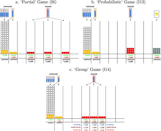
Examples of Representations Used in Games. Panel (a) 'Partial' Game (I6). Panel (b) 'Probabilistic' Game (I13). Panel (c) Group Game (G4).

Notes: Columns represent different states of nature. On the left, the state of nature with no loss shows an income of Q10,000, while the other columns represent states with losses ranging from Q1,000 to Q8,000. Circles indicate frequencies, with four circles representing an event with probability of 1/21. The pictogram (rain gauge or sun) and the shade of the circles indicate weather events: white circles represent normal rainfall, light grey circles heavy rainfall below the threshold for insurance payout, dark grey circles excess rainfall covered by the insurance and medium grey circles incidence of drought. Panel (a) represents a scenario in which normal rainfall occurs with probability 5/7, heavy rainfall with either no loss or Q1,000 loss with probability 1/7 and excessive rainfall with losses of Q3,000, Q5,000, or Q7,000, each with probability of 1/21. In panel (b), the scenario includes a potential loss of Q5,000 with probability 1/7 due to excess rainfall, a potential drought loss of Q8,000 with probability 1/7 and either normal or heavy rainfall with probability 5/7. Panel (c) shows a group game scenario, with alternative rules of risk sharing. If the individual is insured, payment of premium occurs in all states of nature and the payout of Q1,400 occurs in states of excess rainfall in individual games and of the indicated amount for the group risk-pooling scenarios.

To incentivise truthful revelation of WTP, payouts were based on players’ purchase decisions. The first time that participants were shown this visualisation, we conducted a trial run of how their WTP would be linked to their purchase decision. Each farmer having recorded his WTP, the presenter announced a price for the insurance (without disclosure of how it was chosen for this part of the training), which defined who was insured. A random weather event was drawn and each participant drew an associated loss from a deck of cards. Each participant could then complete his form and figure out his net income, and comparison was drawn between those who did and did not purchase the insurance. The exercise was repeated with different possible weather cards. These explanations were followed by a short quiz, with four questions relative to the payout in different cases of rainfall observations and losses, and two questions on group insurance.⁹ Results on the basic concept of index insurance were good, with 59% of subjects having all four answers correct and 84% having at least three correct. On the group insurance, 43% had both answers correct and 86% had at least one correct answer.

Subjects were then notified that, for the remainder of the day’s games, we would record their WTP for each scenario, and then at the end of the day would randomly choose one of the day’s scenarios to be the one on which payouts would be made. For this scenario, we would randomly draw a price and a weather shock, and proceed as just explained. This framed amount of earnings for the season would then be converted to a real payment for the day equal to 0.7% of the framed financial amount. As an example, an individual who would have lost half of a Q10,000 harvest due to excess rainfall in the selected scenario would be paid .007×5,000 = Q35 for the day (in addition to the participation payment) if WTP did not exceed the premium price, and .007×(5,000+ payout − premium) if WTP did exceed the premium price. The maximum payment that they could receive would be Q70, if there was no bad weather shock and they had not purchased the insurance.

The heart of the day’s exercises was a sequence of three games, each one made up of a series of scenarios.¹⁰ The first game was a set of partial insurance scenarios, where we varied the severity and variance of the shocks occurring in the insured state (e.g., variation around the scenario in Figure 1a). These scenarios were used to estimate individual-level utility curves and hence to back out WTP for the other games. The second game presented a set of probabilistic insurance scenarios, in which we introduced a drought risk that hurt income but was not covered by the excess rainfall insurance, and we then varied the severity and likelihood of this drought shock (as in Figure 1b). The third game presented a set of group insurance scenarios (Figure 1c), where the payout was made at the group level and the co-operative could then choose to conduct some loss adjustment to smooth idiosyncratic variation.

Our experiment attempted to probe complex and unfamiliar issues in the course of a single day. Because of this, we decided to design a protocol that was more heavy-handed than is typical in laboratory experiments (the scripts for the exercise are included in their entirety in Online Appendix E). Each scenario was prefaced by three to four sentences that presented how it differed from the previous scenario, and an explanation that pointed to a trade-off, given both an argument while the insurance was valuable (or more valuable than in the previous scenario), and one argument while it was not valuable (or less valuable than in the previous scenario). All introductions were structured with ‘On the one hand . . . On the other hand’. In retrospect, we feel that it may be reasonable to question the balance of the presentation of the scenarios in two out of the 32 cases presented (I2 and I8), one of which is given in the footnote below, but overall we made every effort to ensure that the presentation of the changes across scenarios was even-handed.¹¹ The objective was to help the participants in their decision process without introducing bias.

We report in Appendix C the analysis of three features of the games that were designed to test the robustness of our results to study effects that might threaten internal validity. One is that values on the data entry form were randomised to lie between Q40 and Q320 or Q80 and Q360 to test for bracketing effects. Second, we randomised the order of the games and subsets of scenarios to the maximum extent possible. Third, we tested for the framing effect whereby all experiments were presented with monetary values that correspond to coffee production experiences, but payment at stakes were an order of magnitude different.

1.2. Willingness to Pay

In all scenarios, there are three mutually exclusive states of nature: normal rainfall with no loss, an exogenous set of (excess) rainfall states s ∈ R covered by the insurance and a set of states s ∈ D in which a (heavy rainfall or drought) shock occurs and the index does not trigger, each of which occurs with a given probability.¹² Referring to Figure 1, panel (a) represents a ‘partial’ insurance scenario in which all severe shocks are at least partially covered by the insurance. In panel (b), this ‘probabilistic’ insurance scenario includes a potential insurable loss of Q5,000 with probability 1/7 due to excess rainfall, a potential uninsurable drought loss of Q8,000 with probability 1/7 and either normal or heavy rainfall with probability 5/7. We separately denote the probability of states in which the insurance product will trigger as π_s and states in which a shock occurs but the insurance does not trigger as ω_s. Income is denoted by K when there is no loss, R_s in state s ∈ R and D_s in state s ∈ D. An individual choosing insurance must pay the premium in any state, and if insurance is purchased and the insured states occur then a payout is received. If c is the cost of insurance and P is the payout, the payoff in state s ∈ R is R_s if uninsured and R_s − c + P if insured. For the set of states s ∈ D payoffs are D_s if uninsured and D_s − c if insured. The state in which no shock occurs and no payout occurs happens with frequency 1 − ∑_{s ∈ R}π_s − ∑_{s ∈ D}ω_s and induces payoff K if uninsured and K − c if insured.¹³

Without insurance, an expected utility maximiser will have the following welfare:

\begin{equation*} EU_0=\sum _{s\in R}{\pi _s}u(R_s) + \sum _{s \in D}{\omega _s}u(D_s) + (1- \sum _{s\in R}{\pi _s} - \sum _{s\in D}{\omega _s})u(K). \end{equation*}

(1)

With insurance, expected utility is:

\begin{equation*} EU_I=\sum _{s\in R}{\pi _s}u(R_s+P-c) + \sum _{s\in D}{\omega _s}u(D_s-c) + (1- \sum _{s\in R}{\pi _s} - \sum _{s\in D}{\omega _s})u(K-c). \end{equation*}

(2)

The WTP is the premium payment c that equalises expected utility across these two options.

While the index insurance literature has typically referred to all variation in income that is not covered by the index as ‘basis risk’, there are sharply contrasting theoretical predictions surrounding increases in uncovered risk in insured states versus risk in uninsured states. As the severity of shocks in insured states increases (holding the payout constant), expected utility theory predicts that insurance will become more valuable because its expected marginal utility in the insured states rises. Thus, while the insurance product appears worse in the sense that it covers a smaller fraction of the risk, it should in fact yield a higher WTP. The experimental literature has typically found that demand for partial insurance conforms relatively well to expected utility theory (Wakker et al., 1997), and hence we use the partial insurance game to estimate individual-specific utility curves.

Since the other games effectively represent a relabeling and a reweighting of the same state space used to estimate the utility curves, we can predict what individuals should be willing to pay in any scenario of the other games if the same function drove risk preferences. The difference between this EU-predicted WTP and the actual, observed WTP provides a very clean money-metric measurement of the extent to which demand in more complex risk environments is ‘behavioural’. Specifically, we can also contrast the expected utility environment (in which probabilities enter linearly) with prospect-style utility (Kahneman and Tversky, 1979; Tversky and Kahneman, 1992). In that environment we replace the objective probabilities π_s with decision weights Ω(π_s), which have been found empirically to overemphasise small probabilities and to underweight large probabilities.¹⁴ We confirm that a non-linear weighting of probabilities in our case results in a dramatic over-reaction to small multi-peril risks, and are able to characterise the magnitude of this response with unusual clarity.

When we turn to group insurance demand, the estimation of expected utility WTP again provides us with a benchmark that lets us decompose the various candidate explanations for the demand responses to the collective nature of the group insurance product. We now discuss in detail how the individual-specific utility curves are estimated.

2. Expected Utility and Demand for Partial Insurance

To estimate individual utility curves, we begin from the seven individual scenarios of the partial insurance game, which vary the extent to which the insurance fully covers damages. Their structure is similar to that of I6 represented in Figure 1a. Each of the scenarios presents an environment with five possible (mutually exclusive) states of nature: three states of insurable (excess rainfall) risk with equal probability of occurrence π= 1/21 and income R_s equal to R, R − σ and R + σ, respectively, one state with uninsured (heavy rainfall) shock with probability ω = 1/21 and income D = Q9,000, and one state without loss with probability (1 − 3π − ω) and income K = Q10,000. In the first scenario I1, R = Q7,000 and σ =Q1,000, so that the insurable states correspond to incomes of Q8,000, Q7,000 and Q6,000. In scenarios I2 and I3, we increase the severity of insured shocks (R= Q5,000 and Q3,000, respectively) while keeping their distribution (σ =Q1,000) constant. In scenarios I4 to I7, we keep R = Q5,000 constant, and vary σ in multiple of Q1,000 from 0 to Q3,000. Panel A of Table 1 reports these values.

Table 1.

Summary Statistics on WTP by Game.

Scenarios	Description			Actual willingness to pay	Predicted EU willingness to pay
Panel A: Partial insurance game		R (in Q)	σ (in Q)	(1)	(2)
I1	Partial, small shock	7,000	1,000	24.38	22.73
I2	Partial, medium shock	5,000	1,000	29.51	29.92
I3	Partial, large shock	3,000	1,000	33.87	35.02
I4	Partial, base (no variability)	5,000	0	25.72	28.49
I5	Partial, some variability	5,000	1,000	29.10	29.41
I6	Partial, medum variability	5,000	2,000	32.31	31.42
I7	Partial, large variability	5,000	3,000	35.58	33.40
		Drought risk
Panel B: Probabilistic insurance game		ω	D (in Q)
I4	No drought	0		25.72	28.49
I8	Drought, rare and small	1/21	8,000	21.59	28.05
I9	Drought, rare and medium	1/21	6,000	18.71	26.48
I10	Drought, rare and worst	1/21	2,000	15.58	12.36
I11	Drought, frequent and small	1/7	8,000	17.22	27.24
I12	Drought, frequent and medium	1/7	6,000	14.26	23.50
I13	Drought, frequent and worst	1/7	2,000	11.72	9.86

Notes: WTP are in US$. The exchange rate in 2012 was Q6.30 = US$1.

Using these partial insurance scenarios, we measure how WTP changes with the severity of the shock in the insured state, and hence provide a simple metric of the desire to move income from good states to bad as the bad state gets worse or more frequent. Previous work has suggested that partial insurance demand conforms relatively well to expected utility theory (Wakker et al., 1997),¹⁵ and so we also use the partial insurance scenarios to estimate utility functions.

2.1. Evidence of Risk Aversion and Prudence

We first model risk aversion and prudence in our experimental context, examining how the demand for partial insurance responds to variation in risk. Under the expected utility model, the WTP is solution of:

\begin{eqnarray} EU_0 &\equiv & \sum _s\pi u(R_s) +\omega u(D)+ (1- 3\pi -\omega )u(K) \\ &=&\sum _s\pi u(R_s+P-wtp) +\omega u(D-wtp)+ (1- 3\pi - \omega )u(K-wtp) \equiv EU_I \nonumber. \end{eqnarray}

Total differentiation of the solution equation gives:

\begin{eqnarray} \frac{dwtp}{dR}&=&\frac{1}{EU^{\prime }_I }\sum _s\pi \left[u^{\prime }(R_s+P-wtp)-u^{\prime }(R_s)\right] \\ \nonumber \frac{dwtp}{d\sigma }&=&\frac{1}{EU^{\prime }_I } \pi \left[ -u^{\prime }(R-\sigma +P-wtp) + u^{\prime }(R+\sigma +P-wtp)+ u^{\prime }(R-\sigma )- u^{\prime }(R+\sigma ) \right] \\ \nonumber & \approx & \frac{1}{EU^{\prime }_I } \pi \left[ u^{\prime \prime }(R+P-wtp) -u^{\prime \prime }(R) \right] 2 \sigma. \end{eqnarray}

The first expression confirms that demand falls with the severity of the shock when utility is concave. From the second expression, |$\frac{dwtp}{d\sigma }=0$| if u′ is linear (i.e., u″ is constant). But if preferences exhibit prudence (u‴ > 0), wtp increases with σ.

Panel A of Table 1 presents the average WTP across the partial insurance scenarios. Column 1 shows that WTP increases as the severity of the shocks increases across scenarios I1 to I3, indicating an overall risk aversion among all participants. WTP also increases as the variance in losses increases across scenarios I4 to I7, suggesting the presence of an overall prudence in preference. Hence the behaviour of participants in the partial insurance game is consistent with risk aversion and prudence under expected utility theory.

We now proceed to fit an EU demand model for each individual using these partial insurance scenarios.

2.2. Estimating Utility Functions under EU

The objective of this section is to estimate a utility function for each player based on revealed WTP for the incomplete insurance scheme in the seven partial insurance scenarios I1 to I7. This approach is in spirit similar to Currim and Sarin (1989) and Currim and Sarin (1992) in which the authors calibrate individual behavioural models.

Preferences are represented by the following Power Risk Aversion utility function (Xie, 2000):

\begin{equation*} u(y;k,\beta )=-\frac{1}{k}e^{-k\frac{y^{1-\beta }}{1-\beta }}, \end{equation*}

characterised by two parameters (k, β).

We simplify the expressions for EU given in (1) and (2) with a common notation for all states of nature. Each scenario g presented to the players is characterised by a set of probabilities |$p_{x}^{g}$| for the states of nature with income x and payout |$P_{x}^{g}$| that the insurance will pay if the player is insured (this includes 0 for the uninsured shocks). In a given scenario, the expected utility with and without insurance for an individual with preference parameters (k, β) is:

\begin{eqnarray*} EU_{0}^{g}(k,\beta ) &\equiv & \sum _{x}p_{x}^{g}u(x;k,\beta ), \\ EU_{I}^{g}(k,\beta ,\delta )&\equiv & \sum _x p_{x}^{g}u(x+\delta P_{x}^{g}-c;k,\beta ), \end{eqnarray*}

where δ ∈ [0, 1] is a trust parameter that the agent places on the insurance payout. The addition of the parameter δ is prompted by the fact that observed WTP was in most cases inferior to the actuarially fair price, which is not conceivable with a standard utility function. Our utility estimates are thus identified from variation between scenarios, but not by the overall average expected WTP. The willingness to pay is the solution :

\begin{equation*} wtp(g,\theta )=(c: EU_{I}^{g}-EU_{0}^{g}=0), \end{equation*}

(3)

where θ = (k, β, δ) denotes the vector of parameters of the model.

Despite having only three parameters, this setup is quite flexible. Absolute risk aversion |$ARA=\beta \frac{1}{y}+ky^{-\beta }$| decreases with income for (β > 0 and k > −y^{β − 1}) or (β< 0 and k < −y^{β− 1}), and increases with income otherwise. It converges to the CRRA function |$u(y)=-\frac{1}{k}y^{-k}$| with RRA = k + 1 when β → 1, and is the CARA exponential utility |$u=-\frac{1}{k}e^{-ky}$| with absolute risk aversion k when β = 0. Absolute risk aversion is an increasing function of k and a decreasing function of β, and so are prudence |$(\frac{u^{\prime \prime \prime }}{u^{\prime \prime }})$| and temperance |$(-\frac{u^{\prime \prime \prime \prime }}{u^{\prime \prime \prime }})$|⁠.¹⁶

We proceed now with the estimation of a vector of parameters θ for each individual. We assume that there is some additive measurement error on the willingness to pay, such that the observed willingness to pay by a given individual wtp_g is:

\begin{equation*} wtp_{g}=wtp(g,\theta )+\epsilon _{g}\qquad g=1,\ldots ,7. \end{equation*}

We also assume the usual regularity conditions on the error ϵ_g such that our estimator is consistent and efficient. Let |$\mathbf {X}(\theta )_{G\times 3}$| denote the matrix with characteristic element ∂wtp(g, θ)/∂θ_j, j = 1, 2, 3. For each individual, we use a non-linear least squares estimator:

\begin{equation*} \widehat{\theta }=\arg \min _{\theta \in \Theta }\sum _{g=1}^{G}\left(wtp_{g}-wtp(g,\theta )\right)^{2}, \end{equation*}

(4)

implying that |$\hat{\theta }$| must satisfy the first order conditions:

\begin{equation*} -2\mathbf {X}(\hat{\theta })^{T}\left(\mathbf {wtp}-\mathbf {wtp}(\mathbf {g},\hat{\theta })\right)=\mathbf {0}. \end{equation*}

Equation (4) describes a typical non-linear least squares problem, except that, in addition to being nonlinear, the function wtp(g, θ) is defined only implicitly by equation (3). Thus, the derivatives with respect to θ that define the moment equations, and that are critical to any gradient-based solution algorithm, require application of the implicit function theorem at each trial value of θ.

2.3. Estimated Preferences and Predicted WTP

We start by estimating a unique utility function for all 674 players. Results for the parameters, with robust standard errors clustered at the individual level in parentheses, are reported in Table 2, Col. 1. The utility function exhibits risk aversion and prudence, with absolute risk aversion decreasing only slightly over the range of values of income, from 0.80 to 0.73, implying that relative risk aversion increases very steeply from 1.6 (for the worst income equal to 20% of the normal income) to 7.3 when there is no negative shock to income.

Table 2.

Estimated Parameters of Utility Functions.

	Overall utility	Individual utilities
Parameters	Coeff. (SE)	Median	Lowest 5%	Highest 5%
|$\widehat{ \beta }$|	0.042 (0.120)	0.720	−0.959	3.64
|$\widehat{ k}$|	0.801 (0.194)	0.849	−4.033	50.500
|$\widehat{ \delta }$|	0.156 (0.004)	0.217	0.0737	1.0347

We proceed with the estimation of θ for each individual player. Since we rely on a very small number of observations for each player (at most 7, and less for the 61 players that did not play all 7 scenarios), estimated parameters can take some extreme values. We therefore report the median and the lowest and highest fifth percentile of the estimated parameters in Table 2, Cols. 2–4. We see large variations in estimated parameters across individuals, reflecting heterogeneity in preferences.¹⁷

The estimated utility functions are shown in Figure 2. Using these estimated parameters, we can compute for each individual predicted utility and all of its derivatives at any level of income, and hence average risk aversion and prudence. Among all participants 76% exhibit prudence and 10% have an almost quadratic utility function.

Figure 2.

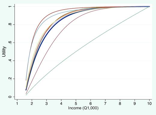
Estimated Individual Utility Functions.

Notes: Utility curves are shown for the different deciles of their distribution, when individuals are ranked according to their risk aversion at the mid-point of the income range. The thick curve is the estimated aggregate utility curve.

For each individual with parameter |$\widehat{\theta }$|⁠, we can compute the predicted WTP, |$\widehat{wtp}(g^{\prime },\widehat{\theta })$|⁠, that the player ought to have for any scenario g′. As above, this is the solution to (3) for that particular scenario characterised by |$p_{x}^{g^{\prime }},P_{x}^{g^{\prime }}$|⁠. The process converged for 621 players for the first three scenarios and 666 players for all other scenarios.

Since measures of risk aversion and |$\widehat{wtp}$| will be used as regressors in the analysis of the observed WTP, we will need some measure of precision on these predicted values to correct the standard errors in the estimations. This is done by implementing a wild bootstrap of the whole procedure, using the six-point distribution proposed by Webb (2013).¹⁸ With equal probability, the residual for each observation is multipled by |$\pm \sqrt{0.5}$|⁠, ±1, or |$\pm \sqrt{1.5}$|⁠. For each replicate we then re-estimate the parameters, and in turn compute the predicted |$\widehat{wtp}(g^{\prime },\widehat{\theta })$| and measure of risk aversion. The wild bootstrap here assumes that errors are independent across observations, but allows them to be heteroscedastic and non-normal. Notice that because it is computationally intensive to repeat the gradient-based search for each bootstrap replicate, the bootstrap parameter estimates rely on a grid search method. The bootstrapped values will be directly used in the estimations that use risk aversion or |$\widehat{wtp}$| as regressors.

3. Demand for Probabilistic Insurance

With these explicit utility functions in hand we now proceed to the analysis of WTP for a set of six probabilistic insurance scenarios.¹⁹ Their structure is similar to that of I13 represented in Figure 1b. Each scenario presents an environment with four possible (mutually exclusive) states of nature: a state with a mild uninsurable shock (with Q1,000 loss and probability 1/21), a dominant state of no shock with high probability, a state of insurable (excess rainfall) shock with probability π = 1/7 and income R = Q5,000, i.e., 50% of potential income K, and a state of uninsurable ‘drought’ shock. The six scenarios vary the probability and intensity of this drought risk. They began with a framing of a mild drought risk—one that was both unlikely to occur (ω = 1/21) and small (loss equal to Q2,000, or 20% of potential income). The magnitude of the drought-induced loss was then increased across scenarios to 40% and 80% of potential income, and then three scenarios were played with the uninsured losses at these same levels but with the probability of this shock being elevated to 1/7. Panel B of Table 1 reports these values and Figure 1b shows I13, the most extreme case of both frequent and severe drought risk. Critically, when the uninsured shock rises to a loss of 80%, it will be the case that the purchase of index insurance will make outcomes in the worst state of nature even worse.

Our goal is to decompose the demand for probabilistic insurance into EU and behavioural components, using the precise measure of what the WTP ‘should’ be if agents were standard expected utility maximisers. This predicted dollar-value WTP under expected utility theory is computed for each participant using his/her own estimated vector of parameter |$\hat{\theta }$| as described in Subsection 2.3. The difference between this amount and the observed WTP provides a monetary estimate of the extent to which decreases in demand for probabilistic insurance are driven by behavioural concerns.

3.1. Comparing the Demand for Probabilistic and Partial Insurance

With partial insurance, payout always occurs in states of shock and hence becomes even more valuable when the severity of the shock increases, as we have shown in Subsection 2.1. In contrast, when the risk is uninsured, the demand for insurance decreases with the severity of the risk, because the utility cost of paying premiums in the shock state goes up.²⁰ We verify these basic relationships in Table 3 by regressing WTP on the standard deviation of residual risk after insurance. In order to assess whether there is a behavioural aspect to the demand for probabilistic insurance, we run the regression for both the observed WTP and the WTP predicted with the EU model. Column 1 shows that the predicted WTP displays the expected relationships; a small uninsurable risk leads to a small decrease in predicted WTP, and more severe shocks in insurable states drives up WTP while more severe shocks in uninsurable states drive it down. Column 2 shows that, as a result, predicted WTP falls by $3.59 when farmers face a mild drought risk, and by $18.80 when they face a risk so severe as to make it possible that the worst state of nature is uninsured.

Table 3.

Willingness to Pay in the Probabilistic Game.

Dependent variable: WTP, US$	Predicted WTP		Actual WTP			Difference actual WTP-predicted WTP
	(1)	(2)	(3)	(4)	(5)	(6)
Any drought	−7.71***		−14.03***
	(0.22)		(0.42)
Residual SD of income in probabilistic game	−79.33***		−31.10***
	(2.63)		(1.14)
Residual SD of income in partial game	62.32***		55.41***
	(2.12)		(2.05)
Mild drought		−3.59***		−12.02***	−10.03***	−8.44***
		(0.11)		(0.38)	(0.35)	(0.34)
Drought inducing the worst possible state		−18.80***		−16.31***	−5.87***	2.48***
		(0.60)		(0.45)	(0.62)	(0.58)
Predicted WTP					0.56***
					(0.03)
Constant	31.91***	30.00***	31.73***	30.03***	13.36***	0.05
	(0.17)	(0.12)	(0.23)	(0.19)	(0.79)	(0.17)
Observations	8,523	8,523	8,547	8,547	8,517	8,517
R-squared	0.795	0.771	0.74	0.704	0.775	0.41

Notes: *** p < 0.01, **p < 0.05, * p < 0.1. Regressions are estimated using scenarios I1-I13. There are fixed effects at the individual level, and standard errors are clustered at the individual level. In Column (5), standard errors bootstrapped from 300 iterations in each of which risk aversion is recalculated to account for the prediction error of the estimated right-hand side variable.

Columns 3 and 4 repeat the previous analysis but using the actual WTP observed across scenarios. While the signs of the responses are consistent, the magnitudes display quite a divergent pattern. Actual WTP proves to be very sensitive to small amounts of drought risk, and then to display little additional sensitivity to the magnitude or likelihood of risk posed by drought (Column 4). This indicates that there is a secular dislike of probabilistic insurance that manifests itself even when the actual probability of uninsurable risk is minimal. To understand how actual and predicted WTP relate to each other, Column 5 runs a regression explaining the former while including the latter as a control variable, and Column 6 uses the simple difference between the two as dependent variable.

The patterns estimated in Table 3 are represented visually in Figure 3, reporting both actual and predicted WTP as function of the residual variance in income after payouts would have occurred. The ‘fitted’ curves are simple quadratic regressions relating the different actual or predicted WTP for the partial or probabilistic insurance games, separately. The clear story emerging from these two ways of analysing the data is that there is a response to small uninsurable risk that cannot be squared with our expected utility predictions, and if anything the surprise in the response to very large uninsurable risk (scenario I13) is that the actual WTP displays less of a decrease than we might expect. Hence, we can conclude very clearly that there is a behavioural dimension in demand that decreases as the probabilistic nature of the insurance is magnified.

Figure 3.

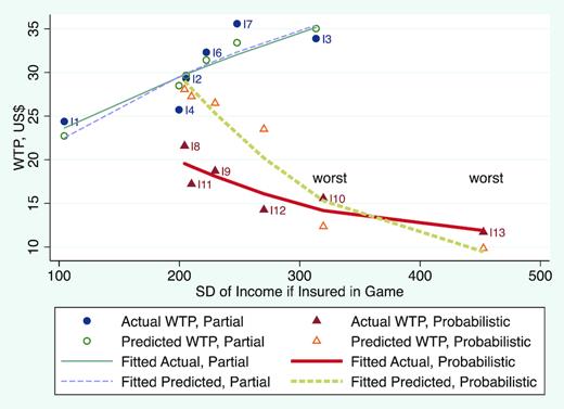
Actual versus Estimated WTP in Partial and Probabilistic Insurance Games.

The literature on probabilistic insurance has compared the demand for insurance when the payout is probabilistic with the standard case of full insurance (Camerer, 2004). In particular, Wakker et al. (1997) show that when the probability of contract failure is small the WTP under EU should be roughly discounted by the probability of contract failure. We conduct a different but closely related exercise, amplifying the probability of an uninsurable loss (and thus shifting the underlying risk profile) while holding the insurance features fixed. We show in Appendix B that under EU the introduction of a small uninsurable shock induces a reduction in WTP that is approximately proportional to the probability ω of the shock, that is:

\begin{equation*} \Delta wtp \simeq \frac{\left[u^{\prime }(K )-u^{\prime }(K-wtp)\right](K-D)}{\pi u^{\prime }(R -wtp+P)+(1-\pi )u^{\prime }(K-wtp) } \omega \lt 0 \end{equation*}

We can refer again to Table 1 to observe how demand is affected by a small probability risk. Scenarios I4, I8 and I11 only differ in the drought risk, with no drought in I4 and a small drought loss with probabilities 1/21 in I8 and 1/7 in I11. Column 2 shows that predicted WTP falls from its value in I4 by $0.43 in I8 and by $1.24 in I11. Change in WTP is thus proportional to the probability of uninsured risk as expected from theory when utility is concave in income and probabilities enter linearly in the EU model. Column 1 shows the actual changes; here by contrast there is a strong response to a very small increase in probability, and then a lower-than-proportional response to increasing the risk further. WTP falls by $4.13, almost 10 times more than under EU, when the probability of drought is set at 1/21, but the decrease in WTP only doubles to $8.50 when the probability of drought is tripled from here. Increasing the magnitude of loss in uninsured states while holding probabilities constant leads to a further decrease in WTP for insurance, a fact that is consistent with concave utility. Consequently, the decision criterion must be concave in income, but non-linear and concave in probabilities over the state space studied here. This result is directly inconsistent with the ‘dual’ theory of Yaari (1987), and also with the rank dependent expected utility theory of Quiggin (1982), since the distortion to decision making (relative to EU) disappears as the magnitude of the low-probability shock increases. It is only consistent with the prospect theory of Kahneman and Tversky (1979) and Tversky and Kahneman (1992).

3.2. Explaining the Behavioural Aversion to Probabilistic Insurance

A major advantage of our cardinal, money-metric measure of the behavioural component of insurance demand is that we can take this as an outcome and explain the difference between the predicted and actual WTP in the mild drought scenarios using a set of individual- and farm-level covariates. The core question we try to answer is the following: is this non-EU component of demand driven by behavioural attributes of the individual, or does it relate to a real risk exposure in their farming activities that makes drought risk more salient?

To address this question, we bring to bear two sets of covariates. The first are behavioural attributes of the individual, including risk aversion, ambiguity aversion, and an index of trust. Ambiguity aversion was measured in the intake survey using four choices between an urn with increasing known probability of winning and an urn with unknown probability of winning. The trust index was built from four questions asking about the extent to which individuals trust their fellow co-operative members.²¹ On the other hand, risk aversion was not elicited with typical survey questions but, to be more consistent with this exercise, computed from the individual-specific utility function estimated as reported in Subsection 2.3. To explain actual risk exposure we rely on a set of survey questions about the main risks facing coffee output on subjects’ farms. We ask about excess rainfall, drought, strong wind, or disease, and we characterise each risk as being relevant at all or being the dominant source of risk for each farmer.

Table 4 presents the results of this analysis. Column 1 shows the simple means of each right-hand side variable. Column 2 uses only the behavioural attributes, and finds that all three of these variables have very strong relationships with the behavioural aversion to probabilistic insurance in the direction that we would expect. The risk averse, for whom insurance is more important overall, are less likely to see large drops in demand as a result of the small drought risk. Similarly, those with a high trust index are less put off by the presence of drought risk and maintain demand. The ambiguity averse, on the other hand show much larger drops in demand when faced with the possibility of mild drought. This latter fact is particularly relevant in that it suggests that the simple survey question eliciting ambiguity aversion does indeed capture relevant information in predicting economically relevant parameters.²²

Table 4.

Deviation from EU Behaviour when Facing Small Uninsured Risk.

	Mean	Reduction in WTP under mild drought risk
	(SD)	Mean value of (predicted WTP - actual WTP) in US$
	(1)	(2)	(3)	(4)	(5)
Behavioural characteristics
Risk aversion	5.76	−0.88***	−0.81**	−0.86**	−0.87**
	(0.80)	(0.35)	(0.36)	(0.36)	(0.37)
Ambiguity aversion	2.2	0.83***	0.85***	0.82***	0.87***
	(1.17)	(0.32)	(0.32)	(0.32)	(0.33)
Trust index	−0.01	−1.00***	−0.95***	−0.95***	−0.88***
	(1.00)	(0.32)	(0.33)	(0.33)	(0.33)
Perceived risk exposure	(Some Risk)		(Some Risk)	(Main Risk)
Excess rainfall	0.91		−0.10	0.41	Dummy
	(0.29)		(1.15)	(1.90)	variables
Drought	0.17		−0.04	2.20	for each
	(0.38)		(0.89)	(2.48)	level
Strong wind	0.24		1.52*	3.66	of each
	(0.43)		(0.79)	(2.91)	risk
Crop disease	0.60		−0.94	0.71
	(0.49)		(0.71)	(2.29)
Constant		11.65***	11.50***	11.02***	16.14**
		(2.47)	(2.68)	(3.08)	(7.14)
Observations	644	644	644	644	644
R-squared		0.036	0.047	0.041	0.064
F_stat. for exposure to risk variables			1.737	0.782	1.089

Notes: *** p < 0.01, ** p < 0.05, * p < 0.1. Risk aversion is the estimated average risk aversion based on the individual-specific utility model. Ambiguity aversion is an indicator from 1 to 5 based on the answers to choices between an urn with increasing known probability of winning and an urn with unknown probability of winning. Trust index is a normalised index of four questions related to trust in the co-op. The risk variables are constructed from responses to the question: Does (Excess rainfall / Drought / Strong Wind / Diseases) represent a risk to your coffee production? Potential answers are: the highest risk, 2nd highest risk, 3rd highest risk, 4th highest risk, no risk. In Columns 1 and 3, the risk variable is set to 0 if answer is no risk, 1 otherwise. In Column 4 the risk is set to 1 if it is the highest risk. In Column 5, there is one variable per type of risk and rank. Standard errors on behavioural characteristics bootstrapped from 300 iterations in each of which risk aversion is recalculated to account for the prediction error of the estimated right-hand side variable.

Columns 3–5 of Table 4 include the actual risk exposure of the farmers to test whether these can explain the over-reaction to small drought risks. Not only is drought exposure insignificant in the first two specifications, and not only does a joint F-test of all four measures of risk exposure prove insignificant both for ‘some’ and for ‘main’ risk, but the point estimates on the behavioural parameters are almost completely unchanged. Even when we dummy out each level of each risk we find the behavioural determinants of this over-reaction to be very robust (Column 5). Taken together, our results show very clearly that this over-response to small risks is driven by the behavioural attributes of the decision-maker and is not driven by the actual exposure to risk.

3.3. Risk Aversion and Demand for Insurance against Severe Risk

We now focus on the response to the ‘worst state’ drought risk. These are scenarios I10 and I13, where the Q8,000 loss suffered in case of drought is more severe than the Q5,000 loss that would be inflicted by excess rainfall, implying that the worst state of nature is not covered by the insurance, and is even made worse by the fact that the premium has to be paid in this state. The literature on demand for index insurance has paid particular attention to this specific type of contract non-performance as a candidate explanation for low demand for index insurance. As shown by Clarke (2016), using an EU model, the possibility of the worst state being uninsured can introduce non-monotonicity into the relationship between risk aversion and insurance demand. The drop in WTP for insurance that features this worst possibility should be particularly pronounced among those with high risk aversion. Similarly, the Maxmin Expected Utility framework used by Gilboa and Schmeidler (1989) and Bryan (2019) evokes a pessimism in which decision-makers fixate on the worst thing that could possibly happen in making insurance purchase decisions, another context in which the effect of these extreme tail risks would be accentuated. Having established that our subjects do not behave according to EU theory in the context of a probabilistic insurance, we revisit this relationship between risk aversion and WTP in our game.

To investigate this, we use data from all the drought scenarios (I8–I13) and I4, the partial insurance scenario with the same insurable risk (but no drought), distinguishing between the severe drought (I10 and I13) and mild drought for the other cases. We interact dummies for mild drought and severe drought with the measure of risk aversion to study the extent to which WTP drops differentially with the risk of severe drought for the most risk averse.

Consistent with the argument in Clarke (2016), Column 1 of Table 5 shows that while mild drought risk leads to differentially higher EU-based predicted WTP among the more risk averse, this relationship flips over with the severe drought, leading to a substantial and differentially lower demand WTP among the more risk averse. In sharp contrast to this, Column 2 illustrates that actual WTP does not differentially decrease in the most severe drought scenarios for the most risk averse (the point estimate is even positive but not significant), even though the premium must be paid in this state. Thus the non-monotonicity in demand over risk aversion as the severity of uninsurable risk increases predicted in the EU model is not observed in actual WTP.

Table 5.

Willingness to Pay and Risk Aversion.

Dependent variable: Willingness to pay, US$	Predicted WTP	Actual WTP
	(1)	(2)
Risk aversion×Mild drought	0.15*	0.33
	(0.10)	(0.58)
Risk aversion×Severe drought	−6.83***	0.7
	(0.97)	(0.63)
Risk aversion	0.99	1.73**
	(0.71)	(0.74)
Mild drought	−3.01***	−9.69***
	(0.63)	(3.20)
Severe drought	21.95***	−16.12***
	(5.67)	(3.75)
Constant	22.80***	15.75***
	(3.90)	(3.85)
Observations	4662	4686
R-squared	0.319	0.142

Notes: *** p < 0.01, ** p < 0.05, * p < 0.1. Regressions are estimated using scenarios I4 and I8-I13. Standard errors bootstrapped from 300 iterations in each of which risk aversion is recalculated to account for the prediction error of the estimated right-hand side variable.

In conclusion, while the overall aversion to insurance featuring large uninsurable risk is largely in line with expected utility theory (Table 3), the mechanism of high risk aversion leading to large drops in WTP does not appear to be the operative one.

4. Demand for Group Insurance

The premise of insuring groups (rather than individuals) is that superior information held by group members allows payouts to be adjusted to reflect the actual losses experienced. Because the smoothing opportunity in group index insurance only occurs in the context of a payout, we only model this scenario in our game and study the way in which the group mechanism can make index insurance less partial. In principle this can permit superior smoothing, and index insurance for aggregate risk can be thought of as complementary to group insurance for idiosyncratic risk (Dercon et al., 2014). Despite this potential, there are important factors that work against group insurance. The group negotiation process is not frictionless, and thus distrust or social costs may make group negotiation an unattractive way to provide smoothing. Even groups that have the capacity to pool risk may fail to do so, and the informality of the typical risk-sharing contract means that issues of contract enforcement and dynamic consistency will be important. Groups may struggle to maintain pooling if the members’ risk exposures are too dissimilar. We now present the results of several experimental scenarios intended to isolate the relative importance of these mechanisms.

The group game presents risk scenarios that are similar to those of the partial insurance scenarios I5–I7, where excess rainfall experienced at the group level may lead to three possible levels of idiosyncratic losses leading to income of R, R − σ and R + σ, where R = Q5,000 now represents the average income in the group. Take the example of G4 represented in Figure 1c, with σ = Q1,000: should there be excess rainfall, individuals within the same group may experience losses of Q4,000, Q5,000 or Q6,000. Hence at the individual level, the risk profile is the same as the individual scenario I5. However, in the group game, should the group be insured, the group will receive an aggregate payout of Q1,400 times the number of insured members. This aggregate payout can then be either equally shared among members or attributed according to experienced losses. In a first set of scenarios, the degree of sharing is pre-specified. In scenario G4-a, there is no sharing and each individual receives Q1,400. In scenario G4-b there is partial sharing and individuals who lost less (more) receive somewhat less (more) than Q1,400. In scenario G4-c there is full sharing and all individuals have after compensation the same average net loss of Q3,600. Similar group scenarios with σ = Q2,000 (G5) and Q3,000 (G6) were also played. Notice that the ability to loss adjust is capped by the size of the payout, so that ‘complete sharing’ is replaced by ‘maximum possible degree of loss adjustment’ in G5-c and G6-c; when insurance is partial then the ability to loss adjust is similarly incomplete.

The group insurance game is played individually. The subject is asked what his WTP for such an insurance would be. The game does not require any co-ordination with the other participants, although it was clearly framed as a potential group insurance for the members of the co-operative to which they all belong, meaning that whatever trust or reservation they have with regard to their co-operative could influence their decision in the game.

The concept of the group insurance was extensively presented in the training session, where we facilitated a discussion in which we explicitly presented the potential for group loss adjustment through unequal sharing of the group payout. A short review preceded the group game exercise.

4.1. The Demand for Group Sharing and the Role of Trust

We begin our analysis of WTP with the results from these tightly framed scenarios in which the within group loss adjustment was specified (scenarios G4–G6). The benchmark case in which no loss adjustment is conducted is exactly comparable to the individual scenarios I5–I7, meaning that the difference in WTP comes from a ‘pure’ preference for the group modality itself. We again use the individual utility curves estimated from the partial insurance game to compute predicted WTP.

Column 1 of Table 6 shows the predicted WTP for group insurance under the three potential levels of risk pooling, as compared to the baseline individual insurance scenario, for the scenarios of low variance (I5 and G4, with σ = Q1,000). By construction, the predicted WTP in the ‘no loss adjustment’ scenario is identical to the individual scenario. The third row of Column 1 shows that the maximal possible risk pooling achievable by the group ought to increase WTP by $7.19. Column 2 shows the same estimation for actual WTP, and provides three fundamental insights into the demand for group risk pooling. The first row illustrates that when farmers are presented with a group index insurance product (G4-a) that is precisely comparable to an individual equivalent (I5), WTP is $5.21 lower. This provides the pure preference for group insurance, demonstrating that all things equal there is a dislike of the group modality and farmers would prefer to be insured individually. We can also compare the changes in the WTP coefficients across the rows of Columns 1 and 2, and here we see that the increase in actual WTP for group insurance as loss adjustment increases to its maximum is $6.07 (0.86 + 5.21), while the predicted WTP increases by slightly more than a dollar more than this. Hence, risk protection that arises from group loss adjustment is slightly less attractive than risk protection that is provided by the insurance company. Finally, while the group becomes more attractive as its degree of loss adjustment increases, the secular dislike of the group mechanism is sufficiently strong that farmers are basically indifferent between even the maximally risk-pooling group insurance mechanism and individual insurance. Column 3 pools all scenarios with low, medium and high variances in risk, and shows that this result is very stable even when we increase the degree of variance in losses.

Table 6.

Willingness to Pay for Group Insurance.

	Amount of loss adjustment conducted by group			Understanding of group insurance	Trust in group		Amount of loss adjustment expected from group
	Predicted WTP	Actual WTP	Actual WTP	Actual WTP	Actual WTP	Actual WTP	Actual WTP	Actual WTP	Actual WTP
Dependent variable: Willingness to Pay, US$	(1)	(2)	(3)	(4)	(5)	(6)	(7)	(8)	(9)
Group with no loss adjustment	0	−5.21***	−5.45***	−6.95***	−5.52***	−5.52***	−5.20***	−5.20***	−5.27***
	(0.00)	(0.52)	(0.47)	(1.12)	(0.47)	(0.47)	(0.50)	(0.46)	(0.46)
Group with moderate loss adjustment	2.11***	−2.25***	−2.17***	−3.68***	−2.25***	−2.25***	−2.23***	−2.15***	−2.24***
	(0.10)	(0.53)	(0.48)	(1.11)	(0.49)	(0.49)	(0.51)	(0.48)	(0.48)
Group with maximal loss adjustment	7.19***	0.86	0.06	−1.45	−0.05	−0.05	0.87	0.07	−0.04
	(0.35)	(0.56)	(0.49)	(1.12)	(0.49)	(0.49)	(0.54)	(0.48)	(0.48)
Medium variance (σ = 2000) in loss			2.85***	2.85***	2.81***	2.82***		3.10***	3.07***
			(0.16)	(0.16)	(0.16)	(0.16)		(0.16)	(0.16)
High variance (σ = 3000) in loss			5.84***	5.84***	5.91***	5.91***		6.32***	6.38***
			(0.23)	(0.23)	(0.23)	(0.23)		(0.24)	(0.25)
Test score×Group game				1.15
				(0.75)
Trust in group×Group game					0.93*	0.90*			0.93*
					(0.51)	(0.52)			(0.50)
Trust×Group×Moderate loss adjustment						0.1
						(0.22)
Trust×Group×Maximal loss adjustment						0.02
						(0.32)
Sharing rule not stipulated							−3.62**	−2.89*	−2.92*
							(1.42)	(1.53)	(1.55)
Trust×Group×Sharing not stipulated									−0.72
									(1.16)
Constant	29.62***	29.27***	29.50***	29.56***	29.43***	29.43***	29.22***	29.21***	29.18***
	(0.11)	(0.38)	(0.34)	(0.34)	(0.35)	(0.35)	(0.44)	(0.50)	(0.52)
Observations	2664	2646	6610	6594	6463	6463	3306	8590	8413
R-squared	0.954	0.744	0.695	0.695	0.685	0.685	0.417	0.392	0.386
Scenarios used	I5, G4abc	I5, G4abc	I5-I7, G4-G6	I5-I7, G4-G6	I5-I7, G4-G6	I5-I7, G4-G6	I5, G1, G4abc	I5-I7, G1-G6	I5-I7, G1-G6
	low variance	low variance	all variances	all variances	all variances	all variances	low variance	all variances	all variances

Notes: *** p < 0.01, ** p < 0.05, * p < 0.1. Regressions include fixed effects at the individual level, and standard errors are clustered at the individual level.

Scenarios G1, G2 and G3 present the same risk profiles as I5, I6 and I7, respectively, as do G4, G5 and G6. All scenarios have the same expected revenue R = Q5000 but varying variance in loss (σ = 1000 in I5, G1 and G4; σ = 2000 in I6, G2 and G5, σ = 3000 in I6, G3 and G6). In G1–G3, the rule of allocation of the group payout is not specified. In G4, G5 and G6, the rule of allocation is specified with no loss adjustment (a), partial loss adjustment (b), or maximum loss adjustment (c) in the group. Columns 1 and 2 only use the scenarios with low variance in loss, Columns 3–6 use all three levels of loss variance. Columns 7–9 also include the three scenarios G1–G3 in which the rule of allocation is not specified. The test score variable is equal to the number of correct answers on the two questions of understanding of group insurance.

What is the origin of this dislike of group insurance? One obvious explanation is that farmers simply do not understand the group game. To test this, we use the score that each individual obtained on two questions relative to group insurance in the quiz taken at the end of the training session. In Column 4 of Table 6, we interact this test score with a dummy for the group scenarios. While individuals with better understanding of group insurance have a higher (though not statistically significant) WTP, even those with the maximum test score of 2 have a reduction in WTP of $4.65 (highly significant with a standard error of 0.67). The next possible interpretation is that farmers do not trust their groups. To test this, we exploit our trust index (described in footnote 21). In Column 5 of Table 6, we interact this trust index with a dummy for the group scenarios. While high-trust individuals do indeed have significantly higher demand for group insurance, the magnitude of this effect is small (93 cents) and hence it would appear that distrust can account for at most about one-fifth of the secular dislike of the group mechanism. Column 6 shows that trust does not alter WTP for the group modality as the level of environmental risk increases. Hence, while trust is not inconsequential, it does not appear to explain the magnitude of the preference for individual insurance.

4.2. How Much Risk Will Groups Actually Choose to Share?

Having understood how much the groups are willing to pay for loss adjustment, we undertook a number of additional experiments to try to unpack some of the most obvious threats to successful group risk sharing, namely (i) how much loss adjustment they believe the group would in fact conduct, (ii) the vulnerability of risk pooling arrangements toex post renegotiation and (iii) the influence that heterogeneity within the group has on the ability to pool risk. In other words, not how much loss adjustment they want, but how much they expect.

To measure the expected degree of loss adjustment, we presented participants with three scenarios G1–G3, in which we asked WTP for a group insurance with exactly the same risk context as G4–G6, but the degree of loss-adjustment left unstipulated. These scenarios were played before any group scenario with stipulated sharing rules. Results are reported in Table 6. In Column 7, we consider the scenarios with small variance in losses (I5, G1 and G4a–c with σ = Q1,000). By comparing WTP in the G1 scenario to the G4 scenarios in which loss adjustment was stipulated, we can measure expectations over pooling in a very exact way. The coefficient on this unstipulated scenario is −$3.62, relative to a coefficient of −$2.23 for a group insurance with moderate pooling and of −$5.20 with no pooling. The implication is that the co-operative members expect that their groups would conduct a fraction of the possible degree of loss adjustment of idiosyncratic risk (corresponding to approximately a quarter of the idiosyncratic risk). Column 8 extends the analysis to all three variance scenarios and arrives at very similar conclusions. Finally, we can ask whether a lack of group trust effects the extent of pooling that the members expect from the group. This is accomplished in Column 9 by interacting group trust with a dummy for the scenario in which the sharing rule was not stipulated; here we see an insignificant effect suggesting that trust is not the driver of expected loss adjustment.

A second issue with group risk pooling is that the contract is not formalised and hence pooling will only occur if those who have the capacity to pay do not seek to renegotiate the contract after shocks have been realised. To try to simulate this possibility in a laboratory context, we conducted a sequenced ‘group deliberation exercise’ described in more detail in Appendix D. We first asked players as individuals what degree of loss adjustment they would prefer (1 = none, 2 = moderate, 3 = as much as possible) if they were obtaining group insurance. We then asked them to discuss and decide upon this issue as a group and recorded the outcome. Finally, we attempted to mimic the incentive to renege on group risk sharing by asking each individual to draw an actual rainfall shock (and thus a level of income) and to vote again on the group risk-pooling decision. On average, the participants report wanting ‘moderate’ risk sharing (50% of potential), both before and after the weather draw, individually and in group.²³ Yet, even in this contrived environment in which individuals are asked to state their preference twice over a very short period of time and with only a small sum of money at stake, we find evidence that the ex post incentive incompatibility of risk pooling will prove problematic. Individuals who draw large negative shocks pivot to desire greater pooling, and those who draw small shocks desire less pooling. The magnitude of the change in behaviour provides some evidence for the extent to which the inability to write binding contracts will pose a constraint on pooling agreements that must be ex post incentive compatible.

Finally, we examined the issue that heterogeneity in expected risk exposure introduces a redistributive element into group risk-pooling contracts, since certain individuals can be expected to be systematically making larger claims on the group than others. Our group heterogeneity analysis, presented in Appendix Table D 2, finds that this is indeed a concern. Simply framing the group as made up of heterogeneous agents causes WTP to drop by $6.54, more than the overall drop from group relative to individual insurance. While WTP changes in the expected direction depending on whether the farmer would on net be making or receiving transfers through the group mechanism, the magnitudes we estimate suggest that when pooling would induce transfers to other group members, WTP falls by only about half as much as it would if the transfer were to the insurance company.

These results provide a mostly negative picture of the demand for group insurance. While farmers do have a strong WTP for loss adjustment via the group mechanism and report wanting to share idiosyncratic risk at 50% of potential, they only expect their groups to loss adjust one-quarter of the potential idiosyncratic variation. Given our evidence that both the dynamic consistency of risk sharing and the heterogeneity of group members is a problem in practice, the expectation that actual risk pooling will come in below the level desired may well be justified.

5. Conclusion and Discussion

Using an artefactual field experiment, we investigate the demand for index insurance among coffee farmers in Guatemala. Willingness to pay is in general lower than the actuarially fair rate, which is an initial piece of evidence that partial insurance products do not generate the kind of demand that we would expect from risk-averse agents if offered perfect insurance. We use the lab context to decompose the potential reasons that insurance products may meet with limited demand and to investigate one promising modality to stimulate demand: co-operative-level loss adjustment combined with index insurance to the group.

Our study provides several novel perspectives on how people respond to risk. First, we can explicitly estimate utility functions from the demand for risk reduction that we believe is well explained by EU theory. This permits us to harness the EU model to predict WTP in a wide variety of counterfactual scenarios, and provides an unusually direct way of decomposing insurance demand. We confirm the very strong role that uninsurable sources of risk play in undermining WTP, and find the drivers of this response to be complex. When the magnitude of uninsurable losses is high, EU responds strongly to the risk and behavioural explanations appear to play very little role in driving the drop in demand. In contrast, even very small and low-probability uninsurable risks have strong effects on WTP. In these cases the EU model would predict only very modest shifts in WTP, and so we find that roughly 90% of the response to small uninsurable risk is behavioural. A prospect-style utility function where the decision criterion is concave in both wealth and probabilities is consistent with these results.

We verify the mechanisms underlying group insurance, but fail to provide much hope that such products will prove commercially viable. Farmers understand the risk-pooling benefits of loss adjustment, and indeed they expect their co-operatives would provide about a quarter of the possible degree of risk pooling. Despite this, there is a secular dislike of the group mechanisms, increasing in the degree of distrust of the co-operative, that makes even a fully loss-adjusted group insurance product only just equal to individual insurance. Given the expected degree of loss adjustment, the average individual would prefer individual insurance to group. Hence, while we verify that the underlying mechanisms that make group insurance potentially attractive are indeed at play, in the end in this context they are insufficient to compensate for the overall dislike of the group mechanism.

Taken together, these results suggest that micro-insurance suppliers bear a substantial burden in terms of creating desirable insurance products and marketing them effectively. Index insurers will struggle to generate demand in environments with multiple risks, and group insurance does not appear to be an attractive way to overcome this hurdle. While insurance demand would rise if climate change caused more severe or more variable shocks in the dimension captured by the index, even a very small increase in risks not covered by the index prove highly detrimental to demand. As uninsured shocks become larger, more likely behavioural explanations become less important, but only because even EU models predict such large decreases in WTP in these scenarios. This study therefore reinforces the need to push index insurance products to cover multi-peril risks, as can be achieved with more sophisticated indexes, or to find ways to directly indemnify agricultural losses.

Additional supporting information may be found in the online version of this article:

Online Appendix

Notes

The authors thank Alain de Janvry for extensive discussions, Eduardo Montoya for research assistance in the estimation of the utility model, Rita Motzigkeit for her help with fieldwork, and Michael Carter and seminar participants at Université d’Auvergne, PSE, and PACDEV for comments. Financial support for this project came from USAID through the Feed the Future Innovation Lab for Assets and Market Access Index Insurance Innovation Initiative (I4) (AEG-A-00-08-00008-00). The contents are the responsibility of the authors and do not necessarily reflect the views of USAID or the US government.

Footnotes

1

All probabilities in our games are explicitly defined, meaning that we study risk but not uncertainty (Ellsberg, 1961).

2

Our environment is not informative as to other behavioural features such as ambiguity aversion (Fox and Tversky, 1995; Bryan, 2019) or the failure to reduce compound lotteries (Segal, 1990; Elabed and Carter, 2015).

3

Dollars are USD throughout (if applicable) .

4

A long line of literature has suggested that in the absence of a formal group dimension to insurance, individual insurance may have a tendency to crowd out informal risk pooling. This has been demonstrated theoretically (Attanasio and Ríos-Rull, 2000) as well as shown in empirical work from India (Mobarak and Rosenzweig, 2014), China (Lin et al., 2014) and Ethiopia (Dercon et al., 2014).

5

Work by Said et al. (2015) suggests that risk-exposed groups may be more sensitive to risk than those who are less exposed.

6

Appendix Table A 2. Given that WTP for insurance is typically found to correlate positively with wealth (Hill et al., 2013), our average WTP may be somewhat overestimated relative to the average co-operative member.

7

The exchange rate in 2012 was Q6.30 = US$1

8

The index is based on cumulative rainfall over the fruiting and flowering period for coffee as measured at the nearest government-administered rainfall station.

9

The questions were as follows: (i) Imagine that you have bought insurance against excess rainfall. The meteorological station does not register excess rainfall. Yet, you lost 25% of your harvest due to rain on your plot. Will you receive a payout from the insurance? (ii) Imagine that two coffee producers, Raul and Lucas, purchased the insurance against excess rainfall. The station registers excess rainfall. Raul lost Q2,000 and Lucas lost Q8,000 due to rain. Do you think that Raul will receive more than Lucas, less than Lucas, or the same as Lucas? (iii) Imagine again that Raul and Lucas have purchased insurance. The station does not register excess rainfall. Raul did not lose any income, but Lucas lost Q3,000. How much will Raul receive: Q0 or Q1,400? (iv) How much will Lucas receive: Q0 or Q1,400? (v) Imagine the company offers group insurance. What would be the price each individual would pay relative to the individual insurance: more, less or the same? (vi) Imagine that you are a member of a group of 10 members that purchased group insurance. In case of excess rainfall, the group will receive Q14,000. If there is excess rainfall, how much would you receive: Q0, Q1,400, or ‘it depends on the decision of the group’?

10

The scenarios will be described in detail as we proceed to analyse them. A summary table of the states of nature presented in each scenario is given in Appendix Table A1.

11

The description for I2 reads: ‘On the one hand, the insurance continues to pay the standard compensation of Q1,400, even though you suffer greater losses than you did previously in the face of excess rainfall. On the other hand, the payout from the insurance is more useful in this scenario than the one before, because it is more difficult to overcome your financial difficulties in years of excess rainfall. Comparing this scenario to the previous one, what is the maximum price you would be willing to pay to purchase this insurance?'

12

The structure of the scenarios is represented in Appendix Figure A 1.

13

For simplicity, we ignore in this formalisation the small loss of $1,000 that may occur with heavy rainfall.

14

We do not have the ability to test standard versus cumulative prospect theory, and hence do not emphasise the difference between these two theories in our presentation. Two other benchmark cases that we will discuss are the ‘Dual’ model of Yaari (1987), in which the weights Ω are non-linear but the utility function u(.) is linear, and the rank dependent expected utility theory of Quiggin (1982), in which only unlikely outcomes that result in extreme changes in utility are overweighted.

15

The authors compare the WTP for three insurance contracts: a standard insurance with no deductible, a 0.99 partial insurance (which pays 99% of any claim), and a 0.99 probabilistic insurance (which pays the full claim 99% time). Under expected utility theory, the WTP for the partial and probabilistic insurance should be approximately 99% of the WTP for the standard insurance. Yet, they find the median ratio of the WTP for the probabilistic insurance to the standard insurance to be as low as 0.50, while it is 0.95 for the partial insurance. This leads them to conclude that demand for partial insurance conforms relatively well with expected utility, but not the demand for probabilistic insurance.

16

The use of a three-parameter utility function to fit seven WTP data points means that R-squared is very high, and concerns about mis-specification are further ameliorated by the fact that we never make out-of-sample predictions because the scenarios in which we predict WTP are conducted over the same state space as those with which we estimate utility curves.

17

The small number of observations imply that standard errors on parameters are extremely high, and the quality of fit of the estimation, measured by |$SSR=\sum _{g=1}^{7}\left(wtp_{g}-wtp(g,\theta )\right)^{2}$|⁠, very good.

18

With fewer than 10 observations, the six-point distribution by Webb is recommended over the more common two-point distribution (Cameron et al., 2011).

19

In essence, all insurance that covers specific sources of risk is probabilistic. The labeling of the uninsured risk as drought was purposefully chosen to highlight this sort of uninsured risk, rather than those unrelated to weather, or to a risk of non-compliance by the insurance company, which would involve other issues besides the existence of uninsured states of the world.

20

Since the insurance product is invariant across all scenarios, these two cases correspond to increasing an uninsurable risk that is positively and negatively correlated with the insurable risk, respectively (Eeckhoudt et al., 1996; Gollier and Pratt, 1996).

21

The questions ask whether the co-operative members trust each other, whether the interest of all members are equally considered when decisions are made, whether rules are respected in decision making, and whether decision making is transparent. For each of these questions, farmers could choose 'Strongly disagree', 'Disagree', 'Agree', 'Strongly Agree', which we coded 1 to 4. The index is the normalised sum of the four scores.

22

To verify that the results are not simply driven by differential understanding of the game, we added controls for the level of education and the result on the quiz of understanding of the rainfall insurance administered to the farmers at the end of the training session. The results were essentially unaffected.

23

See Appendix Table D.1.