


Abstract
Pigmentation has emerged as a premier model for understanding the genetic basis of phenotypic evolution, and a growing catalog of color loci is starting to reveal biases in the mutations, genes, and genetic architectures underlying color variation in the wild. However, existing studies have sampled a limited subset of taxa, color traits, and developmental stages. To expand the existing sample of color loci, we performed QTL mapping analyses on two types of larval pigmentation traits that vary among populations of the redheaded pine sawfly (Neodiprion lecontei): carotenoid-based yellow body color and melanin-based spotting pattern. For both traits, our QTL models explained a substantial proportion of phenotypic variation and suggested a genetic architecture that is neither monogenic nor highly polygenic. Additionally, we used our linkage map to anchor the current N. lecontei genome assembly. With these data, we identified promising candidate genes underlying (1) a loss of yellow pigmentation in populations in the mid-Atlantic/northeastern United States [C locus-associated membrane protein homologous to a mammalian HDL receptor-2 gene (Cameo2) and lipid transfer particle apolipoproteins II and I gene (apoLTP-II/I)], and (2) a pronounced reduction in black spotting in Great Lakes populations [members of the yellow gene family, tyrosine hydroxylase gene (pale), and dopamine N-acetyltransferase gene (Dat)]. Several of these genes also contribute to color variation in other wild and domesticated taxa. Overall, our findings are consistent with the hypothesis that predictable genes of large effect contribute to color evolution in nature.
OVER the last century, color phenotypes have played a central role in efforts to understand how evolutionary processes shape phenotypic variation in natural populations (Gerould 1921; Sumner 1926; Fisher and Ford 1947; Haldane 1948; Cain and Sheppard 1954; Kettlewell 1955). More recently, color variation in nature has begun to shed light on the genetic and developmental mechanisms that give rise to phenotypic variation (True 2003; Protas and Patel 2008; Wittkopp and Beldade 2009; Manceau et al. 2010; Nadeau and Jiggins 2010; Kronforst et al. 2012). A growing catalog of color loci is starting to reveal how ecology, evolution, and development interact to bias the genetic architectures, genes, and mutations underlying the remarkable diversity of color phenotypes (Hoekstra and Coyne 2007; Stern and Orgogozo 2008, 2009; Kopp 2009; Manceau et al. 2010; Streisfeld and Rausher 2011; Martin and Orgogozo 2013; Dittmar et al. 2016; Massey and Wittkopp 2016; Martin and Courtier-Orgogozo 2017). To make robust inferences about color evolution, however, genetic data from diverse traits, taxa, developmental stages, and evolutionary timescales are needed.
Two long-term goals of research on the genetic underpinnings of pigment variation are (1) to evaluate the importance of large-effect loci to phenotypic evolution (Orr and Coyne 1992; Mackay et al. 2009; Rockman 2012; Remington 2015; Dittmar et al. 2016), and (2) to determine the extent to which the independent evolution of similar phenotypes (phenotypic convergence) is attributable to the same genes and mutations (genetic convergence) (Arendt and Reznick 2008; Gompel and Prud’homme 2009; Christin et al. 2010; Manceau et al. 2010; Elmer and Meyer 2011; Conte et al. 2012; Rosenblum et al. 2014). Addressing these questions will require a large, unbiased sample of pigmentation loci. At present, most of what is known about the genetic basis of color variation in animals comes from a handful of taxa and from melanin-based color variation in adult life stages (True 2003; Protas and Patel 2008; Wittkopp and Beldade 2009; Nadeau and Jiggins 2010; Kronforst et al. 2012; Sugumaran and Barek 2016). Another important source of bias stems from a tendency to focus on candidate genes and discrete pigmentation phenotypes [Kopp 2009; Manceau et al. 2010; Rockman 2012; but see Greenwood et al. (2011), O’Quin et al. (2013), Albertson et al. (2014), Signor et al. (2016), Yassin et al. (2016)]. Here, we describe an unbiased, genome-wide analysis of multiple, continuously varying color traits in larvae from the order Hymenoptera, a diverse group of insects that is absent from the current catalog of color loci (Martin and Orgogozo 2013).
More specifically, our study focuses on pine sawflies in the genus Neodiprion. Several factors make Neodiprion an especially promising system for investigating the genetic basis of color variation. First, there is intra- and interspecific variation in many different types of color traits (Figure 1 and Figure 2). Second, previous phylogenetic and demographic studies (Linnen and Farrell 2007, 2008a,b; Bagley et al. 2017) enable us to infer directions of trait change and identify instances of phenotypic convergence in this genus. Third, because many different species can be reared and crossed in the laboratory (Knerer and Atwood 1972; 1973; Kraemer and Coppel 1983; Bendall et al. 2017), unbiased genetic mapping approaches are feasible in Neodiprion. Fourth, a growing list of genomic resources for Neodiprion—including an annotated genome and a methylome for Neodiprion lecontei (Vertacnik et al. 2016; Glastad et al. 2017)—facilitate identification of causal genes and mutations. And finally, an extensive natural history literature (Coppel and Benjamin 1965; Knerer and Atwood 1973) provides insights into the ecological functions of color variation in pine sawflies, which we review briefly for context.
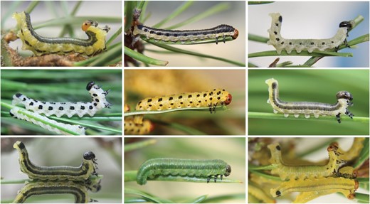
Interspecific variation in Neodiprion larval color. Top row (left to right): Neodiprion nigroscutum, N. rugifrons, N. virginianus. Middle row (left to right): N. pinetum, N. lecontei, N. merkeli. Bottom row (left to right): N. pratti, N. compar, N. swainei. Larvae in the first and last columns are exhibiting a defensive U-bend posture (a resinous regurgitant is visible in N. virginianus, top right). N. pratti photo is by K. Vertacnik, all others are by R. Bagley.
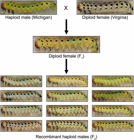
Intraspecific variation in Neodiprion lecontei larval color and cross design. We crossed yellow, light-spotted haploid males from MI to white, dark-spotted diploid females from VA. This produced haploid males with the VA genotype and phenotype (data not shown) and diploid females (F1) with intermediate spotting and color. Virgin F1 females produced recombinant haploid males (F2) with a wide range of body color and spotting pattern (a representative sample is shown).
Under natural conditions, pine sawfly larvae are attacked by a diverse assemblage of arthropod and vertebrate predators, by a large community of parasitoid wasps and flies, and by fungal, bacterial, and viral pathogens (Coppel and Benjamin 1965; Wilson et al. 1992; Codella and Raffa 1993). When threatened, larvae adopt a characteristic “U-bend” posture and regurgitate a resinous defensive fluid (Figure 1), which is an effective repellant against many different predators and parasitoids (Eisner et al. 1974; Codella and Raffa 1995; Lindstedt et al. 2006, 2011). Although most Neodiprion species are chemically defended, larvae vary from a green striped morph that is cryptic against a background of pine foliage to highly conspicuous aposematic morphs with dark spots or stripes overlaid on a bright yellow or white background (Figure 1). Thus, larval color is likely to confer protection against predators either via preventing detection (crypsis) or advertising unpalatability (aposematism) (Ruxton et al. 2004; Lindstedt et al. 2011).
Beyond selection for crypsis or aposematism, there are many abiotic and biotic selection pressures that could act on Neodiprion larval color. For example, insect color can contribute to thermoregulation, protection against UV damage, desiccation tolerance, and resistance to abrasion (True 2003; Lindstedt et al. 2009; Wittkopp and Beldade 2009). Color alleles may also have pleiotropic effects on other traits, such as behavior, immune function, diapause/photoperiodism, fertility, and developmental timing (True 2003; Wittkopp and Beldade 2009; Heath et al. 2013; Lindstedt et al. 2016). Temporal and spatial variation in these diverse selection pressures likely contribute to the abundant color variation in the genus Neodiprion.
As a first step to understanding the proximate mechanisms that generate color variation in pine sawflies, we conducted a QTL mapping study of larval body color and larval spotting pattern in the redheaded pine sawfly, N. lecontei. This species is widespread across eastern North America, where it feeds on multiple pine species. Throughout most of this range, larvae have several rows of dark black spots overlaid on a bright, yellow body (e.g., center image in Figure 1). However, previous field surveys and demographic analyses indicate that there has been a loss of yellow pigmentation in some populations in the mid-Atlantic/northeastern United States and a pronounced reduction in spotting in populations living in the Great Lakes region of the United States and Canada (Bagley et al. 2017; Figure 2). To describe genetic architectures and identify candidate genes underlying these two reduced-pigmentation phenotypes, we crossed white-bodied, dark-spotted individuals from a Virginia population to yellow-bodied, light-spotted individuals from a Michigan population (Figure 2). After mapping larval body-color and spotting-pattern traits in recombinant F2 haploid males, we used our linkage map to anchor the current N. lecontei genome assembly and identified candidate color genes within our QTL intervals. We conclude by comparing these initial findings on color genetics in pine sawflies with published studies from other insect taxa.
Materials and Methods
Cross design
To investigate the genetic basis of sawfly color traits, we crossed N. lecontei females from a white-bodied, dark-spotted population (collected from Valley View, VA; 37°54’47”N, 79°53’46”W) to N. lecontei males from a yellow-bodied, light-spotted population (collected from Bitely, MI; 43°47’46”N, 85°44’24”W). Both populations were collected from the field in 2012 and reared on Pinus banksiana (jack pine) for at least two generations in the laboratory via standard rearing protocols [described in more detail in Harper et al. (2016) and Bendall et al. (2017)]. Our mapping families were derived from four grandparental pairs, which produced 10 F1 females. Like most hymenopterans, N. lecontei adults reproduce via arrhenotokous haplodiploidy, in which unfertilized eggs develop into haploid males and fertilized eggs develop into diploid females (Heimpel and de Boer 2008; Harper et al. 2016). Therefore, to produce an F2 haploid generation, we allowed virgin F1 females to lay eggs and reared their haploid male progeny on P. banksiana foliage until they reached a suitable size for phenotyping.
Color phenotyping
N. lecontei larvae pass through five (males) or six (females) feeding instars and a single nonfeeding instar (Benjamin 1955; Coppel and Benjamin 1965; Wilson et al. 1992). For phenotyping, we chose only mature feeding larvae. For both sexes, mature larvae have an orange-red head capsule with a black ring around each eye and up to four pairs of rows of black spots (Wilson et al. 1992). After phenotyping, we preserved each larva in 100% ethanol for molecular work. In total, we generated color-phenotype data for 30 individuals from the VA population (mixed sex), 30 individuals from the MI population (mixed sex), 47 F1 females, and 429 F2 males (progeny of 10 virgin F1 females).
Larval body color:
We quantified larval body color in two ways: spectrometry and digital photography. First, we immobilized larvae with CO2 and recorded 15 reflectance spectra—five measurements from each of three body regions: the dorsum, lateral side, and ventrum—using a USB2000 spectrophotometer with a PX-2 Pulsed Xenon light source and SpectraSuite software (Ocean Optics, Largo, FL). We then used the program CLR: Color Analysis Programs v1.05 (Montgomerie 2008) to trim the raw reflectance data to 300–700 nm, compute 1-nm bins, and to compute the following summary statistics [described in more detail in the CLR documentation, Montgomerie (2008)]: B1, B2, B3, S1R, S1G, S1B, S1U, S1Y, S1V, S3, S5a, S5b, S5c, S6, S7, S8, S9, H1, H3, H4a, H4b, and H4c. This procedure produced 15 estimates for each summary statistic for each larva, which we then averaged to obtain a single value per statistic per larva. To reduce the 22 color summary statistics to a smaller number of independent variables, we performed a principal component analysis (PCA). To ensure that each variable was normally distributed, we performed a normal-quantile transformation prior to performing the PCA. Based on examination of the resulting scree plot, we retained the first two principal components (PC1 and PC2), which together accounted for 73.7% of the variance in the spectral data. Based on factor loadings, PC1 (percent variance explained: 48.2%) corresponds to saturation (S1G, S1Y, S8) and brightness (B1, B2), whereas PC2 (percent variance explained: 25.5%) corresponds to saturation (S5A, S5B, S5C, S6) and hue (H4c) (Supplemental Material, Table S1 in File S1). Unless otherwise noted, the PCA and all other statistical analyses were performed in R [version 3.1.3 or 3.2.3, R Core Team (2013)].
Because it provides objective and information-rich data, spectrometry is generally considered to be the gold standard for color quantification (Endler 1990; Andersson and Prager 2006). However, despite efforts to keep background lighting and reflectance probe positioning as consistent as possible across samples, measurement of small patches of yellow on rounded larval bodies proved challenging. Given the potential for variation in reflectance probe position to introduce substantial noise into our data (Montgomerie 2006), we used digital photography as a complementary method for quantifying larval body color (Stevens et al. 2007). For this analysis, we photographed CO2-immobilized larvae (dorsal and lateral surfaces) with a Canon EOS Rebel t3i camera equipped with an Achromat S 1.0X FWD 63 mm lens and mounted on a copy stand. All photographs were taken in a dark, windowless room, and larvae were illuminated by two SLS CL-150 copy lamp lights, each with a 23-W (100 W equivalent) soft white compact fluorescent light bulb. We then used Adobe Photoshop CC 2014 or 2015 (Adobe Systems Incorporated, San Jose, CA) to ascertain the amount of yellow present, following O’Quin et al. (2013). First, we converted each digital image (lateral surface) to CMYK color mode. Next, we selected the eye-dropper tool (set to a size of 5 × 5 pixels) as the color sampler tool, which we used to sample three different body locations: the body just behind the head and parallel to the eye, the first proleg, and the anal proleg. For each of the three regions, this procedure yielded an estimate of the proportion of the selected area that was yellow. We then averaged the three measurements to produce a single final measurement of yellow pigmentation (hereafter referred to as “yellow”).
Larval spotting pattern:
On each side, N. lecontei larvae have up to four rows of up to 11 spots extending from the mesothorax to the ninth abdominal segment (Wilson et al. 1992). We quantified the extent of this black spotting in two ways: the number of spots present (spot number) and the proportion of body area covered by spots (spot area). To quantify spot number, we counted the number of spots in digital images of the dorsal and lateral surfaces (one side only). To quantify larval spotting area, we used Adobe Photoshop’s quick selection tool to measure the area of the larval body (minus the head capsule) and the area of each row of lateral black spots. To control for differences in larval size, we divided the summed area of all lateral black spots by the area of the larval body. We also used Adobe Photoshop to calculate the area of the head capsule, which we used as a covariate in some analyses to control for larval size (see below). We used a custom Perl script to process measurement output files in bulk (written by John Terbot II; available in File S3).
Statistical analysis of phenotypic data:
In total, we produced three measures of body color (PC1, PC2, and yellow) and two measures of spotting pattern (spot number and spot area). To determine whether mean phenotypic values for the five color traits differed between the two populations and among the three generations of our cross, we performed Welch’s two-tailed t-tests, followed by Bonferroni correction for multiple comparisons. To determine the extent to which these five traits covaried in the F2 males, we calculated Pearson’s correlation coefficients (r) and associated P-values, followed by Bonferroni correction for multiple comparisons. To determine which covariates to include in our QTL models, we performed ANOVAs to evaluate the relationship between each phenotype in the F2 males (429 total) and their F1 mothers (10 total) and head capsule sizes (a proxy for larval size/developmental stage).
Genotyping
We extracted DNA from ethanol-preserved larvae using a modified CTAB method (Chen et al. 2010) and prepared barcoded and indexed double-digest RAD libraries using methods described elsewhere (Peterson et al. 2012; Bagley et al. 2017). We prepared a total of 10 indexed libraries: one consisting of the eight grandparents and 10 F1 females (18 adults total), and the remaining nine consisting of F2 haploid male larvae (∼48 barcoded males per library). After verifying library quality using a Bioanalyzer 2100 (Agilent, Santa Clara, CA), we sent all 10 libraries to the University of Illinois Urbana-Champaign Roy J. Carver Biotechnology Center (Urbana, IL), where the libraries were pooled and sequenced using 100-bp single-end reads on two Illumina HiSeq2500 lanes. In total, we generated 400,621,900 reads.
We demultiplexed and quality-filtered raw reads using the protocol described in Bagley et al. (2017). We then used Samtools v0.1.19 (Li et al. 2009) to map our reads to our N. lecontei reference genome (Vertacnik et al. 2016) and STACKS v1.37 (Catchen et al. 2013) to extract loci from our reference alignment and to call SNPs. We called SNPs in two different ways. First, for QTL mapping analyses, our goal was to recover fixed differences between the grandparental lines. To do so, we first called SNPs in our eight grandparents and 10 F1 mothers. For these 18 individuals, we required that SNPs had a minimum of 7× coverage and no more than 12% missing data. We then compiled a list of SNPs that represented fixed differences and, as an additional quality check, confirmed that all F1 females were heterozygous at these loci. We then used STACKS to call SNPs in the F2 haploid males, requiring that each SNP had a minimum of 5× coverage, no more than 10% missing data, and was present in the curated list produced from the grandparents. Filtering in STACKs produced 559 SNPs genotyped in 429 F2 males.
Second, to maximize the number of SNPs available for genome scaffolding, we performed an additional STACKS run using only the F2 haploid males, requiring that each SNP had a minimum of 4× coverage. By removing the requirement that SNPs were called in all grandparents, we could recover many more SNPs. We then filtered the data in VCFtools v0.1.14 (Danecek et al. 2011) to remove individuals with a mean depth of coverage <1, retaining 408 F2 males. After removing low-coverage individuals, we used VCFtools to remove sites with a minor allele frequency <0.05, sites with >5 heterozygotes (in a sample of haploid males, high heterozygosity is a clear indication of pervasive genotyping error), and sites with >50% missing data.
Linkage map construction and genome scaffolding
To construct a linkage map for interval mapping, we started with 559 SNPs scored in 429 F2 males. After an additional round of filtering in R/qtl (Broman and Sen 2009), we removed 11 haploid males that had >50% missing data, for a total of 418 F2 males. Additionally, after removing SNPs that were genotyped in <70% of individuals, had identical genotypes to other SNPs, and had distorted segregation ratios (at α < 0.05, after Bonferroni correction for multiple testing), we retained 503 SNPs. To assign these markers to linkage groups, we used the “formLinkageGroups” function, requiring a minimum logarithm of odds (LOD) score of 6.0 and a maximum recombination frequency of 0.35. To order markers on linkage groups, we used the “orderMarkers” function, with the Kosambi mapping function to allow for crossovers, followed by rippling on each linkage group.
Our initial map included 503 SNPs spread across 358 scaffolds (out of 4523 scaffolds; Vertacnik et al. 2016). To increase the number of scaffolds that we could place on our linkage groups, we performed linkage mapping analyses with a larger SNP dataset that was generated as described above. For each of our four grandparental families (N = 54, 73, 120, and 161), we first performed additional data filtering in R/qtl to remove duplicate SNPs and SNPs with distorted segregation ratios, retaining between 2049 and 3155 SNPs per family. We then used the “formLinkageGroups” command with variable LOD thresholds (range: 5–15) and a maximum recombination frequency of 0.35. Because SNPs were not coded according to grandparent of origin, many alleles were switched. We therefore performed an iterative process of linkage group formation, visualization of pairwise recombination fractions and LOD scores (“plotRF” command), and allele switching (“switchAlleles” command) until we obtained seven linkage groups (the number of N. lecontei chromosomes; Smith 1941; Maxwell 1958; Sohi and Ennis 1981) and a recombination/LOD plot indicative of linkage within, but not between linkage groups. Because marker ordering for these larger panels of SNPs was prohibitively slow in R/qtl, we used the more efficient MSTmap algorithm, implemented in R/ASMap v0.4-7 (Taylor and Butler 2017), to order our markers along their assigned linkage groups.
Finally, to order and orient our genome scaffolds along linkage groups (chromosomes), we used ALLMAPS (Tang et al. 2015) to combine information from our five maps (initial map with all individuals, but limited markers; plus four additional maps, each with more markers, but fewer individuals). Because maps constructed from large families are likely to be more accurate than those constructed from small families, we weighted the maps according to their sample sizes.
Interval mapping analysis
To map QTL for our five color traits, we used R/qtl and the linkage map estimated from 503 SNPs and 418 F2 males. We included F1 mothers and head-capsule size as covariates in our analyses of PC1, spot number, and spot area; F1 mothers as covariates in our analysis of PC2; and no covariates in in our analysis of yellow (Table S2 in File S1). For each trait, we performed interval mapping using multiple imputation mapping. We first used the “sim.geno” function with a step size of 0 and 64 replicates. We then used the “stepwiseqtl” command to detect QTL and select the multiple QTL model that optimized the penalized LOD score (Broman and Sen 2009; Manichaikul et al. 2009). To obtain penalties for the penalized LOD scores, we used the “scantwo” function to perform 1000 permutations under a two-dimensional, two-QTL model that allows for interactions between QTL and the “calc.penalties” function to calculate penalties from these permutation results, using a significance threshold of α = 0.05. Finally, for each QTL retained in the final model, we calculated a 1.5 LOD support interval.
Candidate gene analysis
As a first step to moving from QTL intervals to causal loci, we compiled a list of candidate color genes and determined their location in the N. lecontei genome. For larval spotting, we included genes in the melanin synthesis pathway and genes that have been implicated in pigmentation patterning (Wittkopp et al. 2003; Protas and Patel 2008; Wittkopp and Beldade 2009; Sugumaran and Barek 2016). For larval body color, we included genes implicated in the transport, deposition, and processing of carotenoid pigments derived from the diet (Palm et al. 2012; Yokoyama et al. 2013; Tsuchida and Sakudoh 2015; Toews et al. 2017). Although several pigments can produce yellow coloration in insects (e.g., melanins, pterins, ommochromes, and carotenoids), we focused on carotenoids because a heated pyridine test (McGraw et al. 2005) was consistent with carotenoid-based coloration in N. lecontei larvae (Figure S1 in File S1).
We searched for candidate genes by name in the N. lecontei v1.0 genome assembly and NCBI annotation release 100 (Vertacnik et al. 2016). To find missing genes and as an additional quality measure, we obtained FASTA files corresponding to each candidate protein and/or gene from NCBI (using Apis, Drosophila melanogaster, or Bombyx mori sequences, depending on availability). We then used the i5k Workspace@NAL (Poelchau et al. 2014) BLAST (Altschul et al. 1990) web application to conduct tblastn (for protein sequences) or tblastx (for gene sequences) searches against the N. lecontei v1.0 genome assembly, using default search settings. After identifying the top hit for each candidate gene/protein, we used the WebApollo (Lee et al. 2013) JBrowse (Skinner et al. 2009) N. lecontei genome browser to identify the corresponding predicted protein coding genes (from NCBI annotation release 100) in the N. lecontei genome.
We took additional steps to identify genes in the yellow gene family, all of which contain a major royal jelly protein (MRJP) domain (Ferguson et al. 2011). First, we used the search string “major royal jelly protein Neodiprion” to search the NCBI database for all predicted yellow-like and yellow-MRJP-like N. lecontei genes. We then downloaded FASTA files for the putative yellow gene sequences (26 total). Next, we used the Hymenoptera Genome Database (Elsik et al. 2016) to conduct a blastx search of our N. lecontei gene sequence queries against the Apis mellifera v4.5 genome NCBI RefSeq annotation release 103. Finally, we recorded the top A. mellifera hit for each putative N. lecontei yellow gene.
Data availability
Short-read DNA sequences ae available in the NCBI Sequence Read Archive (Bioproject PRJNA434591). The linkage-group anchored assembly (N. lecontei genome assembly version 1.1) is available via NCBI (Bioproject PRJNA280451) and i5k Workspace@NAL (https://i5k.nal.usda.gov/neodiprion-lecontei). File S3 contains the custom script used to process the raw spot-area data. File S4 contains phenotypic data from all generations. File S5 contains the input file for R/qtl. File S6 and File S7 contain the genotype data and linkage maps used in the scaffolding analysis.
Results and Discussion
Variation in larval color traits
Laboratory-reared larvae derived from the two founding populations differed significantly from one another for all color phenotypes (Figure 2, Figure 3, and Table S3 in File S1). Because larvae were reared on the same host under the same laboratory conditions, these results suggest that genetic variance contributes to variance in these larval color traits. Crosses between the VA and MI lines produced diploid F1 female larvae that were intermediate in both body color and spotting pattern (Figure 2 and Figure 3). F1 larvae differed significantly from both grandparents for all color traits except PC2 (Table S3 in File S1), indicating a lack of complete dominance for most traits. We can make additional inferences about trait dominance by comparing the phenotypes of diploid F1 female larvae (dominance effects present) to those of the haploid F2 male larvae (dominance effects absent). For all three body-color measures (yellow, PC1, and PC2), average F1 larval colors were more MI-like (yellow) than those of F2 larvae. In contrast, compared to the F2 larvae, F1 spotting phenotypes (number and area) were more similar to the VA population (dark-spotted). Overall, these data suggest that the more heavily pigmented body-color and spotting-pattern phenotypes (i.e., large values for yellow, spot number, and spot area; small values for PC1 and PC2) are partially dominant to the less pigmented phenotypes.
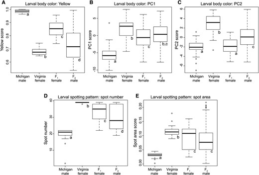
Larval color variation among N. lecontei populations and across generations. For larval body color (A–C), higher scores for yellow (A) and lower scores for PC1 (B) and PC2 (C) indicate higher levels of yellow pigment. For larval spotting pattern (D–E), higher spot numbers (D) and spot area scores (E) indicate more melanic spotting. For all traits, boxes represent interquartile ranges (median ± 2 SD), with outliers indicated as points. For each trait (A–E), lowercase letters indicate which comparisons differ significantly after correction for multiple comparisons (see Table S3 in File S1 for full statistical results).
Larval color variation in the F2 males spanned—and even exceeded—the range of variation in the grandparental populations and F1 females (Figure 3). Recapitulation of the grandparental body-color and spotting-pattern phenotypes in the F2 males suggests that both types of traits are controlled by a relatively small number of loci. There are multiple, nonmutually exclusive explanations for the transgressive color phenotypes in our haploid F2 larvae, including variation in the grandparental lines, reduced developmental stability in hybrids, epistasis, unmasking of recessive alleles in haploid males, and the complementary action of additive alleles from the two grandparental lines (Rieseberg et al. 1999).
We also observed significant correlations between many of the color traits (Figure S2 in File S1). Encouragingly, estimates of body color derived from digital images (yellow) correlated significantly with both estimates derived from spectrometry (PC1 and PC2), suggesting that these independent data sources describe the same underlying larval color phenotype (i.e., amount of yellow pigment). Similarly, we observed strong correlations between the number and area of larval spots, indicating that both measures reliably characterize the extent of melanic spotting on the larval body. We also found that larvae with yellower bodies (small values for PC2) tended to be less heavily spotted (Figure S2 in File S1). However, the correlation between these traits was weak and we observed many different combinations of spotting and pigmentation in the recombinant F2 males (Figure 2).
Linkage mapping and genome scaffolding
Our 503 SNP markers were spread across seven linkage groups, which matches the number of N. lecontei chromosomes (Smith 1941; Maxwell 1958; Sohi and Ennis 1981). The total map length was 1169 cM, with an average marker spacing of 2.4 cM and maximum marker spacing of 24.3 cM (Figure 4 and Table S4 in File S1). Together, these results indicate that this linkage map is of sufficient quality and coverage for interval mapping. With a genome size of 340 Mb (estimated via flow cytometry; C. Linnen, unpublished data), these mapping results yielded a recombination density estimate of 3.43 cM/Mb. This recombination rate is lower than estimates from social hymenopterans, which have among the highest recombination rates in eukaryotes (Wilfert et al. 2007). Nevertheless, our rate estimate is on par with other (noneusocial) hymenopterans, which lends support to the hypothesis that elevated recombination rates in eusocial hymenopteran species is a derived trait and possibly an adaptation to a social lifestyle (Gadau et al. 2000; Schmid-Hempel 2000; Crozier and Fjerdingstad 2001).
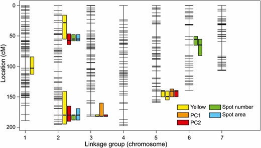
N. lecontei linkage map with larval color QTL and 1.5 LOD support intervals.
Linkage maps estimated for the four grandparental families, each of which contained >2000 markers, ranged in length from 1072 to 3064 cM (Table S4 in File S1). Variation in map length is likely attributable to both decreased mapping accuracy in smaller families and decreased genotyping accuracy in these less-stringently filtered SNP datasets. Nevertheless, marker ordering was highly consistent across linkage maps (Figures S3–S9 in File S1). Additionally, via including more SNPs, we more than tripled the number of mapped scaffolds (from 358 to 1005) and increased the percentage of mapped bases from 41.2 to 78.9% (Tables S5–S6 in File S1). Using this information, we updated the current N. lecontei genome assembly in NCBI and i5k Workspace@NAL (see Data availability). Anchored genome scaffolds, coupled with existing N. lecontei gene annotations, are a valuable resource for identification of candidate genes within QTL.
Genetic architectures of larval body color and larval spotting pattern
Combining the results from our three measures of larval body-color (yellow, PC1, and PC2), our interval mapping analyses detected a total of six distinct QTL regions and one QTL × QTL interaction (Figure 4, Figure 5A, and Table 1). Of these, the largest-effect QTL were on linkage groups 3 and 5. We also recovered a significant interaction between these QTL for yellow (Figure 5B). Compared to analyses of larval body color, analyses of larval spotting pattern yielded fewer distinct QTL (four), but more QTL × QTL interactions (three) (Figure 4, Figure 5, C and D, and Table 1). Both spotting measures (spot number and spot area) recovered two large-effect QTL on LG 2. These spotting QTL also overlapped with QTL with small-to-modest effects on body color (Figure 4 and Table 1). Colocalization of spotting pattern and body color QTL suggests that the phenotypic correlations we observed between body color and spotting pattern in F2 males (Figure S2 in File S1) are caused by underlying genetic correlations via either pleiotropy or physical linkage.
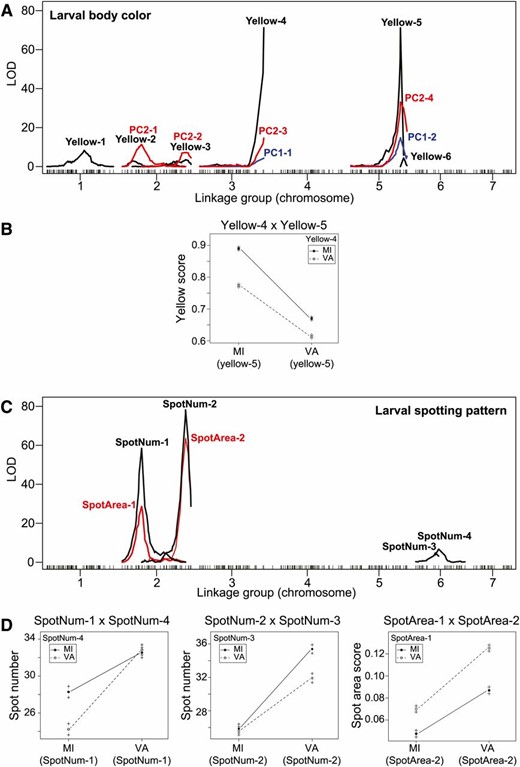
LOD profiles and interaction plots for larval color traits. Interval mapping analyses recovered QTL for larval body color (Yellow, PC1, PC2) on linkage groups 1, 2, 3, and 5 (A) and a single QTL × QTL interaction (B). QTL for larval spotting pattern (spot area and spot number) were on linkage groups 2 and 6 (C), with three QTL × QTL interactions (D). QTL names are as in Table 1.
QTL locations and effect sizes for larval body color (yellow, PC1, and PC2) and larval spotting pattern (spot number and spot area)
| Trait type | Trait | QTL name | Linkage groupa | Position (interval)b | Markerc | LOD | % variance explained | Effect size (SE)d | % Differencee |
|---|---|---|---|---|---|---|---|---|---|
| Body color | Yellow | Yellow-1 | 1 | 105.9 (84.4–112.5) | 5,744 | 8.29 | 1.32 | −0.025 (0.0043) | 8.06 |
| Body color | Yellow | Yellow-2 | 2 | 28.2 (16.2–55.1) | 19,162 | 2.92 | 0.45 | −0.014 (0.0043) | 4.63 |
| Body color | Yellow | Yellow-3 | 2 | 179.9 (140.8–194.0) | 15,279 | 3.51 | 0.54 | −0.016 (0.0043) | 5.13 |
| Body color | Yellow | Yellow-4 | 3 | 181.9 (179.8–181.9) | 1,882 | 71.23 | 16.27 | −0.084 (0.0043) | 27.19 |
| Body color | Yellow | Yellow-5 | 5 | 140.6 (139.9–149.6) | 3,222 | 71.17 | 16.25 | −0.16 (0.0081) | 51.64 |
| Body color | Yellow | Yellow-6 | 5 | 149.6 (140.6–154.8) | 19,661 | 4.37 | 0.68 | −0.035 (0.0082) | 11.43 |
| Body color | Yellow | Interaction | Yellow-3 × Yellow-5 | 12.45 | 2.03 | 0.061 (0.0086) | 19.58 | ||
| Body color | PC1 | PC1-1 | 3 | 181.9 (160.4–181.9) | 1,882 | 4.31 | 3.56 | 1.15 (0.26) | 15.51 |
| Body color | PC1 | PC1-2 | 5 | 140.6 (137.4–149.6) | 3,222 | 14.75 | 12.92 | 2.17 (0.26) | 29.30 |
| Body color | PC2 | PC2-1 | 2 | 55.1 (46.8–63.9) | 21 | 11.37 | 6.42 | 1.18 (0.16) | 23.46 |
| Body color | PC2 | PC2-2 | 2 | 179.8 (165.2–189.9) | 2,143 | 7.24 | 3.99 | 0.91 (0.16) | 17.99 |
| Body color | PC2 | PC2-3 | 3 | 181.9 (179.8–181.9) | 1,882 | 14.60 | 8.39 | 1.33 (0.16) | 26.39 |
| Body color | PC2 | PC2-4 | 5 | 140.6 (139.9–149.6) | 3,222 | 33.13 | 21.13 | 2.09 (0.16) | 41.45 |
| Spotting pattern | Spot number | SpotNum-1 | 2 | 55.1 (48.0–57.6) | 9,282 | 58.46 | 23.52 | 6.31 (0.36) | 33.06 |
| Spotting pattern | Spot number | SpotNum-2 | 2 | 179.9 (179.8–187.5) | 15,279 | 78.19 | 35.45 | 7.81 (0.35) | 40.96 |
| Spotting pattern | Spot number | SpotNum-3 | 6 | 55.7 (51.1–64.9) | 9,040 | 4.84 | 1.43 | −0.58 (0.59) | 3.05 |
| Spotting pattern | Spot number | SpotNum-4 | 6 | 64.9 (55.7–82.2) | 7,485 | 6.75 | 2.02 | −1.00 (0.59) | 5.26 |
| Spotting pattern | Spot number | Interaction | SpotNum-1 × SpotNum-4 | 6.15 | 1.84 | 3.45 (0.71) | 18.09 | ||
| Spotting pattern | Spot number | Interaction | SpotNum-2 × SpotNum-3 | 4.64 | 1.38 | −3.13 (0.71) | 16.39 | ||
| Spotting pattern | Spot area | SpotArea-1 | 2 | 55.1 (48.0–57.6) | 9,282 | 28.62 | 12.99 | 0.029 (0.0025) | 34.86 |
| Spotting pattern | Spot area | SpotArea-2 | 2 | 179.9 (169.1–187.5) | 15,279 | 63.73 | 35.47 | 0.048 (0.0024) | 57.04 |
| Spotting pattern | Spot area | Interaction | Spot-1 × Spot-2 | 1.76 | 0.69 | 0.014 (0.0049) | 16.49 |
Linkage group number.
Position in centimorgan (1.5 LOD support intervals)
Marker closest to QTL peak.
Effect sizes calculated as the difference in the phenotypic averages of among F2 males carrying a VA allele and F2 males carrying an MI allele (± SE).
Effect sizes calculated as a percentage of the difference between average trait values for the two grandparental lines (VA and MI).
| Trait type | Trait | QTL name | Linkage groupa | Position (interval)b | Markerc | LOD | % variance explained | Effect size (SE)d | % Differencee |
|---|---|---|---|---|---|---|---|---|---|
| Body color | Yellow | Yellow-1 | 1 | 105.9 (84.4–112.5) | 5,744 | 8.29 | 1.32 | −0.025 (0.0043) | 8.06 |
| Body color | Yellow | Yellow-2 | 2 | 28.2 (16.2–55.1) | 19,162 | 2.92 | 0.45 | −0.014 (0.0043) | 4.63 |
| Body color | Yellow | Yellow-3 | 2 | 179.9 (140.8–194.0) | 15,279 | 3.51 | 0.54 | −0.016 (0.0043) | 5.13 |
| Body color | Yellow | Yellow-4 | 3 | 181.9 (179.8–181.9) | 1,882 | 71.23 | 16.27 | −0.084 (0.0043) | 27.19 |
| Body color | Yellow | Yellow-5 | 5 | 140.6 (139.9–149.6) | 3,222 | 71.17 | 16.25 | −0.16 (0.0081) | 51.64 |
| Body color | Yellow | Yellow-6 | 5 | 149.6 (140.6–154.8) | 19,661 | 4.37 | 0.68 | −0.035 (0.0082) | 11.43 |
| Body color | Yellow | Interaction | Yellow-3 × Yellow-5 | 12.45 | 2.03 | 0.061 (0.0086) | 19.58 | ||
| Body color | PC1 | PC1-1 | 3 | 181.9 (160.4–181.9) | 1,882 | 4.31 | 3.56 | 1.15 (0.26) | 15.51 |
| Body color | PC1 | PC1-2 | 5 | 140.6 (137.4–149.6) | 3,222 | 14.75 | 12.92 | 2.17 (0.26) | 29.30 |
| Body color | PC2 | PC2-1 | 2 | 55.1 (46.8–63.9) | 21 | 11.37 | 6.42 | 1.18 (0.16) | 23.46 |
| Body color | PC2 | PC2-2 | 2 | 179.8 (165.2–189.9) | 2,143 | 7.24 | 3.99 | 0.91 (0.16) | 17.99 |
| Body color | PC2 | PC2-3 | 3 | 181.9 (179.8–181.9) | 1,882 | 14.60 | 8.39 | 1.33 (0.16) | 26.39 |
| Body color | PC2 | PC2-4 | 5 | 140.6 (139.9–149.6) | 3,222 | 33.13 | 21.13 | 2.09 (0.16) | 41.45 |
| Spotting pattern | Spot number | SpotNum-1 | 2 | 55.1 (48.0–57.6) | 9,282 | 58.46 | 23.52 | 6.31 (0.36) | 33.06 |
| Spotting pattern | Spot number | SpotNum-2 | 2 | 179.9 (179.8–187.5) | 15,279 | 78.19 | 35.45 | 7.81 (0.35) | 40.96 |
| Spotting pattern | Spot number | SpotNum-3 | 6 | 55.7 (51.1–64.9) | 9,040 | 4.84 | 1.43 | −0.58 (0.59) | 3.05 |
| Spotting pattern | Spot number | SpotNum-4 | 6 | 64.9 (55.7–82.2) | 7,485 | 6.75 | 2.02 | −1.00 (0.59) | 5.26 |
| Spotting pattern | Spot number | Interaction | SpotNum-1 × SpotNum-4 | 6.15 | 1.84 | 3.45 (0.71) | 18.09 | ||
| Spotting pattern | Spot number | Interaction | SpotNum-2 × SpotNum-3 | 4.64 | 1.38 | −3.13 (0.71) | 16.39 | ||
| Spotting pattern | Spot area | SpotArea-1 | 2 | 55.1 (48.0–57.6) | 9,282 | 28.62 | 12.99 | 0.029 (0.0025) | 34.86 |
| Spotting pattern | Spot area | SpotArea-2 | 2 | 179.9 (169.1–187.5) | 15,279 | 63.73 | 35.47 | 0.048 (0.0024) | 57.04 |
| Spotting pattern | Spot area | Interaction | Spot-1 × Spot-2 | 1.76 | 0.69 | 0.014 (0.0049) | 16.49 |
Linkage group number.
Position in centimorgan (1.5 LOD support intervals)
Marker closest to QTL peak.
Effect sizes calculated as the difference in the phenotypic averages of among F2 males carrying a VA allele and F2 males carrying an MI allele (± SE).
Effect sizes calculated as a percentage of the difference between average trait values for the two grandparental lines (VA and MI).
These genetic mapping results provide us with our first glimpse of the genetic architecture of naturally occurring color variation in pine sawflies. For both larval body color and larval spotting pattern, we recovered a relatively small number of loci, some of which had a substantial effect on the color phenotype (Table 1). Additionally, our multiple-QTL models explained a considerable percentage of the observed variation in larval color: up to 86% for larval body color (yellow) and up to 73% for larval spotting pattern (spot number) (Table 2). Although limited statistical power precluded us from quantifying the number of QTL of very small effect, our results suggest that the proportion of variation explained by small, isolated QTL is small. It is possible, however, that our large-effect QTL comprise many linked QTL of individually small effect (e.g., Stam and Laurie 1996; McGregor et al. 2007; Bickel et al. 2011; Linnen et al. 2013). Distinguishing between oligogenic architectures (a small number of moderate to large-effect loci) and polygenic architectures (a large number of small-effect loci) will require fine-mapping and functionally validating genes and mutations for both color traits. Nevertheless, for both types of color traits, our results clearly rule out both a monogenic architecture and an architecture in which there are many unlinked, small-effect mutations. The latter architecture is also highly unlikely if gene flow accompanied local color adaptation in pine sawflies (Griswold 2006; Yeaman and Whitlock 2011), as previous demographic analyses seem to indicate is the case (Bagley et al. 2017).
Summary of full multiple-QTL models for five larval color traits
| Trait type | Trait | Covariates | No. of QTL | No. of interactions | LOD | % variance explained |
|---|---|---|---|---|---|---|
| Body color | Yellow | None | 6 | 1 | 182.03 | 85.83 |
| Body color | PC1 | Size, mother | 2 | 0 | 27.14 | 25.48 |
| Body color | PC2 | Mother | 4 | 0 | 65.84 | 50.92 |
| Spotting pattern | Spot number | Size, mother | 4 | 2 | 122.18 | 73.23 |
| Spotting pattern | Spot area | Size, mother | 2 | 1 | 94.77 | 63.93 |
To date, QTL-mapping and candidate-gene studies of color traits have yielded many examples of simple genetic architectures in which one or a small number of mutations have very large phenotypic effects (Rockman 2012; Martin and Orgogozo 2013). However, the relevance of these studies to broader patterns in phenotypic evolution remains unclear due to biases that stem from a tendency to work on discrete phenotypes and specific candidate genes. These biases can be minimized by focusing on continuously varying color traits and employing an unbiased mapping approach as we have done here [see also Greenwood et al. (2011), O’Quin et al. (2013), Albertson et al. (2014), Signor et al. (2016), Yassin et al. (2016)]. Experimental biases aside, some have also argued that color itself—but not color pattern—is atypically genetically simple (Charlesworth et al. 1982; Rockman 2012). In our own data, we see no obvious differences between the architectures of body color and spotting pattern. If anything, the architecture of spotting appears slightly simpler (fewer QTL with larger individual effects) than that of body color (Table 1). That said, more spotting variation remains unexplained (Table 2), which could be attributable to a plethora of undetected small-effect loci, and thus a more complex underlying architecture. A more definitive test of the color/pattern hypothesis will require fine-mapping our QTL, with the prediction that the spotting QTL will fractionate to a greater extent (i.e., break into more QTL of individually smaller effect) than the body color QTL. A rigorous evaluation of the color/pattern hypothesis will also require data on the genetic architectures of color and pattern traits that have evolved independently in other taxa. To this end, ample variation in both body color and color pattern traits make Neodiprion sawflies an ideal system for determining whether there are predictable differences in the genetic architectures of different types of color traits.
Candidate genes for larval color traits
In total, we identified 61 candidate genes with known or suspected roles in melanin-based or carotenoid-based pigmentation and for which we were able to identify putative homologs in the N. lecontei genome (Table S7 in File S2). Of these, 26 appeared to belong to the yellow gene family. Notably, this number is equivalent to the number of yellow-like/yellow-MRJP-like genes found in the genome of the jewel wasp, Nasonia vitripennis, which boasts the highest reported number of yellow-like genes of any insect to date (Werren et al. 2010). Additionally, 13 of these genes (yellow-e, yellow-e3, four yellow-g, yellow-h, yellow-x, and five MJRPs) were found in tandem array along three adjacent scaffolds (548, 170, and 36; ∼1 Mb total) on linkage group 2. This genomic organization is consistent with a conserved clustering of yellow-h, -e3, -e, -g2, and –g found in Apis, Tribolium, Bombyx, Drosophila, and Nasonia (Drapeau et al. 2006; Werren et al. 2010; Ferguson et al. 2011). Like Nasonia and Apis, this cluster also contains MJRPs; like Heliconius, this cluster contains a yellow-x gene. Overall, we placed 57 of our 61 color genes on our linkage-group anchored assembly. With these data, we identified candidate genes for all but two QTL (Yellow-1 on linkage group 1 and SpotNum-3 on linkage group 6) (Table S7 in File S2).
Candidate genes for larval body color:
Both of our largest-effect body color QTL regions contained promising candidate genes with known or suspected roles in carotenoid-based pigmentation (Table S7 in File S2). First, in the linkage group 3 QTL region (Yellow-4, PC1-1, PC2-3; Figure 4 and Table 1), we found a predicted protein-coding region with a high degree of similarity to the B. mori Cameo2 scavenger receptor protein (e-value: 1 × 10⁻¹⁸; bitscore: 92.8). Cameo2 encodes a transmembrane protein that has been implicated in the selective transport of the carotenoid lutein from the hemolymph to specific tissues (Sakudoh et al. 2010; Tsuchida and Sakudoh 2015). In the silkworm B. mori, Cameo2 is responsible for the C mutant phenotype, which is characterized by a combination of yellow hemolymph and white cocoons that arises as a consequence of disrupted transport of lutein from the hemolymph to the middle silk gland (Sakudoh et al. 2010; Tsuchida and Sakudoh 2015).
Second, in the linkage group 5 QTL region (Yellow-5, Yellow-6, PC1-2, PC2-4; Figure 4 and Table 1), we recovered a predicted protein coding gene with a high degree of similarity to the ApoLTP-1 and ApoLTP-2 protein subunits (encoded by the gene apoLTP-II/I) of the B. mori lipid transfer particle (LTP) lipoprotein (e-value: 0; bitscore: 391). LTP is one of two major lipoproteins present in insect hemolymph and appears to be involved in the transport of hydrophobic lipids (including carotenoids) from the gut to the other major lipoprotein, lipophorin, which then transports lipids to target tissues (Tsuchida et al. 1998; Palm et al. 2012; Yokoyama et al. 2013). Based on these observations, we hypothesize that loss-of-function mutations in both Cameo2 and apoLTP-II/I contribute to the loss of yellow pigmentation in white-bodied N. lecontei larvae.
Candidate genes for larval spotting pattern:
Our two largest-effect spotting pattern QTL also yielded promising candidate genes—this time in the well-characterized melanin biosynthesis pathway (Table S7 in File S2). In both linkage group 2 QTL regions, we found protein-coding genes that belong to the yellow gene family. The first linkage group 2 QTL region (SpotNum-1 and SpotArea-1; Figure 4 and Table 1) contained two yellow-like genes that were most similar to Apis yellow-x1 (e-value: 1.2 × 10−160; bitscore: 471.47 and e-value: 3.9 × 10−151; bitscore: 448.36). At present, there is little known about the function of yellow-x genes, which appear to be highly divergent from other yellow gene families (Ferguson et al. 2011). The second linkage group 2 QTL region (SpotNum-2 and SpotArea-2; Figure 4 and Table 1) contained a cluster of 13 yellow genes, including yellow-e. In two different mutant strains of B. mori, mutations in yellow-e produced a truncated gene product that results in increased pigmentation in the head cuticle and anal plate compared to wild-type strains (Ito et al. 2010). Thus, one possible mechanism for the reduced spotting observed in the light-spotted MI population is an increase in yellow-e expression.
The second linkage group 2 spotting QTL region also contained a predicted protein that was highly similar to tyrosine hydroxylase (TH) (e-score: 6 × 10−123, bitscore: 406). TH (encoded by the gene pale) catalyzes the hydroxylation of tyrosine to 3,4-dihydroxyphenylalanine, a precursor to melanin-based pigments (Wright 1987). Work in the swallowtail butterfly Papilio xuthus and the armyworm Pseudaletia separata demonstrates that TH and another enzyme, dopa decarboxylase, are expressed in larval epithelial cells containing black pigment (Futahashi and Fujiwara 2005; Ninomiya and Hayakawa 2007). Furthermore, inhibition of either enzyme prevented the formation of melanin-based larval pigmentation patterns (Futahashi and Fujiwara 2005). Thus, a reduction in the regional expression of pale is another plausible mechanism underlying reduced spotting in the light-spotted MI population.
We also found candidate genes in some of our QTL of more modest effect. As noted above, the Yellow-2 and Yellow-3 QTL overlap with the two large-effect spotting QTL (Figure 4, Figure 5, and Table 1). One possible explanation for this observation is that genes in the melanin biosynthesis pathway impact overall levels of melanin throughout the integument and therefore overall body color. Finally, the SpotNum-4 QTL contained a gene encoding dopamine N-acetyltransferase (Dat). Dopamine N-acetyltransferase, which catalyzes the reaction between dopamine and N-acetyl dopamine and ultimately leads to the production of a colorless pigment, is responsible for a difference in pupal case color between two Drosophila species (Ahmed-Braimah and Sweigart 2015).
Comparison with color loci in other taxa:
Identification of candidate genes in our QTL peaks provides an opportunity to compare our results with those from other insect taxa. For melanin-based traits, the bulk of existing genetic studies involve Drosophila fruit flies (Massey and Wittkopp 2016), with a handful of additional studies in wild and domesticated lepidopterans (e.g., Ito et al. 2010; Van’t Hof et al. 2016; Nadeau et al. 2016). A recent synthesis of Drosophila studies suggests that cis-regulatory changes in a handful of genes controlling melanin biosynthesis (yellow, ebony, tan, Dat) and patterning (bab1, bab2, omb, Dll, and wg) explain much of the intra- and interspecific variation in pigmentation (Massey and Wittkopp 2016). Although our data cannot speak to the contribution of cis-regulatory vs. protein-coding changes, we do recover some of the same melanin biosynthesis genes (yellow and Dat). By contrast, all of the Drosophila melanin patterning genes fell outside of our spotting pattern QTL intervals (Table S7 in File S2). Although we cannot rule these genes out completely, our results suggest that none of them plays a major role in this intraspecific comparison. Whether the same is true of patterning differences within and between other Neodiprion species remains to be seen.
Compared to melanin-based pigmentation, little is known about the genetic underpinnings of carotenoid-based pigmentation, which is widespread in nature (Heath et al. 2013; Toews et al. 2017). Nevertheless, studies in the domesticated silkworm (Sakudoh et al. 2010; Tsuchida and Sakudoh 2015), salmonid fish (Sundvold et al. 2011), and scallops (Liu et al. 2015) collectively suggest that scavenger receptor genes such as our candidate Cameo2 may be a common and taxonomically widespread source carotenoid-based color variation (Toews et al. 2017). Beyond evaluating patterns of gene reuse, extensive intra- and interspecific variation in larval body color across the genus Neodiprion (Figure 1) has the potential to provide novel insights into the molecular mechanisms underlying carotenoid-based pigmentation.
Summary and conclusions
Our study, which focuses on naturally occurring color variation in an undersampled life stage (larva), taxon (Hymenoptera), and pigment type (carotenoids), represents a valuable addition to the invertebrate pigmentation literature. Our results also have several implications for both hymenopteran evolution and color evolution. First, we provide the first recombination-rate estimate for the Eusymphyta, the sister group to all remaining Hymenoptera (e.g., bees, wasps, and ants) (Peters et al. 2017). Our estimate suggests that the exceptionally high recombination rates observed in some social hymenopterans represents a derived state, supporting the hypothesis that increased recombination is an adaptation for increasing genetic diversity in a colony setting (Gadau et al. 2000; Schmid-Hempel 2000; Crozier and Fjerdingstad 2001; Wilfert et al. 2007). Second, for both larval body color and spotting pattern, we can conclude that intraspecific variation is due neither to a single Mendelian locus nor to a large number of unlinked, small-effect loci. However, it remains to be seen whether color, color pattern, and other types of phenotypes differ predictably in their genetic architectures (Dittmar et al. 2016; Rockman 2012). Third, our QTL intervals contain several key players in melanin-based and carotenoid-based pigmentation in other taxa, including yellow, Dat, and Cameo2 (Massey and Wittkopp 2016; Toews et al. 2017). Although functional testing is needed to establish causal links, we can rule out a major role for several core melanin-patterning genes in this intraspecific comparison. Finally, although much work remains—including fine-mapping QTL, functional analysis of candidate genes, and genetic dissection of diverse color traits in additional Neodiprion populations and species—our rapid progression from phenotypic variation to strong candidate genes demonstrates the tremendous potential of this system for addressing fundamental questions about the genetic basis of color variation in natural populations.
Acknowledgments
For assistance with collecting and maintaining sawfly colonies, we thank past members of the Linnen laboratory, especially Robin Bagley, Adam Leonberger, Kim Vertacnik, Mary Collins, and Aubrey Mojesky. For assistance with phenotypic data collection, we thank Aubrey Mojesky, Mary Collins, and Ismaeel Siddiqqi. For advice on linkage mapping in R/qtl, we thank Karl Broman and Kelly O’Quin. For constructive comments on earlier versions of this manuscript, we thank Danielle Herrig, Emily Bendall, Kim Vertacnik, Katie Peichel, and two anonymous reviewers. For assistance with NCBI submissions, we thank Scott Geib. For computing resources, we thank the University of Kentucky Center for Computational Sciences and the Lipscomb High Performance Computing Cluster. Funding for this research was provided by the National Science Foundation (DEB-1257739; to C.R.L.), the United States Department of Agriculture National Institute of Food and Agriculture (2016-67014-2475; to C.R.L.), the Academy of Finland (project no. 257581; to C.L.), and the University of Kentucky (Ribble summer undergraduate research fellowship, honors program independent research grant, and summer research and creativity fellowship to T.S.).
Footnotes
Supplemental material is available online at www.genetics.org/lookup/suppl/doi:10.1534/genetics.118.300793/-/DC1.
Communicating editor: K. Peichel
Literature Cited
Vertacnik, K. L., S. Geib, and C. R. Linnen, 2016 Neodiprion lecontei genome assembly Nlec1.0, NCBI/GenBank. Available at: http://dx.doi.org/10.15482/USDA.ADC/1235565. Accessed: 11/04/2016
Author notes
Present address: Department of Biological Sciences, University of Cincinnati, Cincinnati, OH 45221.
