A simple method for earthquake location by surface-wave time reversal

SUMMARY

The scalar 2-D Helmholtz equation (i.e. ‘membrane waves’) can be used to model surface-wave propagation in a laterally smooth, lossless half-space. Building on this known result, we develop an algorithm to localize earthquake sources based on surface-wave data, via numerical time reversal on a membrane, where monochromatic waves propagate with the phase velocity of Rayleigh or Love waves at the same frequency. By conducting monochromatic membrane-wave time-reversal simulations at various frequencies and combining the results, broad-band time-reversed surface waves can be modelled. Importantly, membrane-wave modelling is computationally much less expensive than 3-D surface-wave modelling. We first explain rigorously the relationship between surface waves and membrane waves. Our mathematical treatment is slightly different from those found in the literature, in that it does not invoke variational principles. We next implement our time-reversal algorithm via spectral elements as well as simple ray tracing. Both implementations account for the effects of lateral variations in phase velocity. We validate the two resulting tools by means of several numerical experiments. This includes synthetic tests, as well as the localization of a virtual source based on a data set of real ambient-noise cross-correlations, and the localization of the epicentre of a real earthquake from real, raw data. In this study, applications are limited to northern Italy and the Alpine arc, where we have access to recent, high-resolution phase velocity maps, ambient-noise cross-correlations and data from a recent, relatively large earthquake. The accuracy of epicentre location despite non-uniformity in station coverage encourages further applications of our method, in particular to the task of mapping large-earthquake rupture in space and time.

Earthquake dynamics, Earthquake source observations, Theoretical seismology, Wave propagation

1 INTRODUCTION

Estimates of seismic slip as a function of position and time for a given earthquake are obtained today in different ways, depending on the magnitude and depth of the earthquake, and on the instrumental coverage. Several different types of seismic and geodetic observations are employed. Dense networks of strong-motion accelerometers are currently deployed in seismic regions worldwide; they are designed to record the high-frequency oscillations generated by a nearby event, but they have little sensitivity to the lower frequencies, and cannot be used to constrain the properties of far earthquakes. At the opposite end of the frequency spectrum, data from GPS networks and satellite geodesy are used as constraints of the final slip associated with an earthquake; they provide good resolution of the surface expression of the rupture, but have little or no sensitivity to fault geometry at depth (e.g. Mai et al.2016,and references therein). Wherever the coverage provided by nearby instruments is insufficient, local and/or global broad-band seismic networks at teleseismic distances are used to image slip. As a general rule, fault geometry is particularly hard to constrain on the basis of seismic data alone, and is determined based on geodetic data or, wherever possible, field geology observations.

Once a data set for a given event has been compiled, seismic oscillations and geodetic offsets are translated to slip on the fault via (1) least-squares inversions, (2) seismic time reversal, or (3) the back-projection method.

1. Least-squares inversions are based on the representation theorem (e.g. Aki & Richards 2002), that is, the mathematical expression of the physical law relating the geometry of an arbitrary rupture to the resulting deformation at any point of a given medium. Because the spatiotemporal evolution of seismic ruptures is generally very complex, it is not surprising that their solutions tend to be very non-unique, as shown in detail by Mai et al. (2016).

2. The physics of acoustic or seismic time reversal can be heuristically summarized as follows: a signal is emitted by a source and recorded by multiple receivers; if receivers are then turned into sources, each emitting its own recorded signal (with the corresponding delay) flipped with respect to time, the resulting wave field will ‘focus’ at the original source location (e.g. Fink 1999). This means that by recording real data from an unknown source and then conducting the time-reversal exercise numerically, the location of the source could be determined, provided, of course, that the error associated with modelling of propagation is small, that is to say, that the complexity of the medium of propagation is accounted for within a good approximation. From the standpoint of seismology, this amounts to a kinematic, extended-source inversion, with the additional possibility of monitoring the backward propagation of time-reversed waves before focusing at the source. In seismology, applications of time reversal (e.g. Larmat et al.2006, 2008) are hindered by the high computational costs of accurate wave-propagation modelling, unless only very long periods are considered.

3. The back-projection method as described, for example, by Ishii et al. (2005) and currently employed by many authors in seismology, is usually thought of as a simplification of wavefield reverse-time migration, a tool for imaging structure in reflection seismology. This is in many ways similar to time reversal, but involves some further, fundamental simplifications. Namely, the term back-projection refers to studies where the effects of time-reversed wave propagation are not modelled, but approximately corrected for by stacking the signals recorded by an array of nearby receivers. One of the practical consequences of this is that the physical nature of the computed, time-reversed wave field that focuses at the source remains undefined. Its interpretation in terms of rupture mechanics is complicated by the fact, for example, that it is not known whether it more closely approximates a slip or a rate of slip (Fukahata et al.2014).

We provide in this study the building blocks of a new algorithm for constraining extended-source geometry and time evolution. The algorithm is based on the time-reversal concept, and thus overcomes the limitations of P-wave back-projection, but it is designed so as to reduce significantly the computational costs of full-waveform time reversal. One of the key aspects of our method is that surface waves, instead of P waves, are time-reversed and backward-propagated. This is preferable for several reasons: (i) Surface waves are dispersive, that is, they ‘spread out’ along the time axis as they travel across the surface of the earth: time reversal turns this process around, enhancing the focusing of backward-propagating waves onto the source. (ii) The problem of surface-wave propagation modelling, although inherently 3-D, can be reduced to 2-D by separating the signal into narrow frequency bands (e.g. Tanimoto 1990; Tromp & Dahlen 1993; Peter et al.2007, 2009), to be back-projected separately, and subsequently ‘stacked’ together: this reduces the computational costs drastically. (iii) Our knowledge of the 3-D structure of the Earth’s deep interior, essential to backward-propagate numerically the time-reversed signal, is limited; but surface-wave propagation is confined to the upper mantle, which is relatively well known; recent, robust global phase-velocity maps of Rayleigh- and Love-wave velocities are available in the frequency band relevant to this project at the global and, where possible, regional scales (e.g. Ekström 2011; Kaestle et al.2018). In seismology/acoustics jargon, point (iii) is equivalent to saying that very accurate surface-wave ‘Green’s functions’ are available and will be used to backward-propagate time-reversed surface-wave data. This further enhances focusing of the time-reversed wave field, and thus the robustness and resolution of mapped seismic slip.

We expect our method to be effective over a broad range of epicentral distances. At distances of 30° or more from the epicentre, surface waves carry more energy than body waves, and they can be easily identified and isolated on seismograms. At shorter epicentral distances, where they are obscured by the body-wave coda, surface waves can still emerge in a time-reversal exercise as a result of focusing: this is confirmed by our results, discussed in Section 6.3.

Today, broad-band ‘full-waveform’ information is not routinely utilized by researchers interested in mapping the seismic source. Tentative implementations of fault imaging via seismic-waveform time reversal such as those by Larmat et al. (2006, 2008) were successful from a theoretical standpoint, but seem too computationally heavy for systematic practical application. Most seismologists only back-project seismogram peaks associated with the arrival of P waves (e.g. Ishii et al.2005) so as to avoid costly simulations of broad-band seismic-wave propagation in a heterogeneous, 3-D medium (the Earth), whose heterogeneity is only approximately known. The only published experiment in surface-wave back-projection that we are aware of is that of Roten et al. (2012). While the basic idea of Roten et al. (2012) is similar to some of the concepts presented here, their approach is essentially a form of back-projection, with the inherent approximations.

We provide in Section 2 a description of surface-wave propagation in terms of ‘potentials’ (e.g. Udías 1999; Aki & Richards 2002). Aki & Richards (2002) state (box 7.5) that ‘potentials are of no direct interest, and are awkward to use. . .’. We maintain that, as shown, for example, by Tanimoto (1990) or Peter et al. (2007), there is interest in using potentials, particularly for surface waves. For instance, if only the phase, and not the amplitude, of the data is studied, many useful applications (e.g. imaging, backward propagation) become possible by using the potentials and the associated simple, 2-D equations, without having to solve the more cumbersome radial equations, or the general 3-D equations. This is strictly true within a high-frequency approximation, but applications to real data have often shown that, in practice, this approximation works remarkably well. Our theoretical formulation in Section 2 is different from that of Aki & Richards (2002) in that we use potentials, and from those of Tanimoto (1990) and Tromp & Dahlen (1993) in that we do not invoke variational principles.

The main implication of Section 2 is that the scalar 2-D Helmholtz equation can be used to model surface-wave propagation in a laterally smooth, lossless half space, confirming earlier results by Tanimoto (1990) and Tromp & Dahlen (1993). In Sections 3 and 4 we accordingly derive the theory of time reversal in a 2-D ‘acoustic’ medium (i.e. a medium whose deformations are described by the 2-D Helmholtz equation). Finally (Section 6), theoretical results are validated by direct application to synthetic and real surface-wave data. The applications presented here are limited to 2-D; in future work, we shall explore the resolving power of our method in the vertical direction, combining the results of multiple, Love- and Rayleigh-wave 2-D time-reversal simulations conducted at different frequencies.

2 SURFACE WAVES AND THE 2-D HELMHOLTZ EQUATION

The scalar 2-D Helmholtz equation can be used to model surface-wave propagation in a laterally smooth, lossless half space. We shall give a simplified proof of this fundamental result by briefly summarizing some parts of earlier studies by Tanimoto (1990) and Tromp & Dahlen (1993). Let us start by writing the displacement equation for an elastic, isotropic medium in the frequency (ω) domain (Udías 1999,eq. 2.60),

\begin{equation*} \frac{\partial }{\partial x_j} \left[ \lambda \delta _{ij} \frac{\partial u_k}{\partial x_k} + \mu \left(\frac{\partial u_i}{\partial x_j} + \frac{\partial u_j}{\partial x_i} \right) \right] = - \rho \omega ^2 u_j, \end{equation*}

(1)

where x₁, x₂, x₃ are Cartesian coordinates, with the x₃-axis perpendicular to Earth’s surface (which we assume to be flat) and oriented downward; δ_ij is Kronecker’s delta, ρ denotes density and λ, μ Lamé’s parameters. Repeated indices are implicitly summed over. Following Tanimoto (1990), we assume the Earth to be smooth laterally (horizontal derivatives of ρ, λ, μ, etc. are negligible) but not vertically (x₃-derivatives of the same parameters are not negligible); eq. (1) then takes a slightly different form for i = 3 with respect to i = 1,2; namely

\begin{equation*} ( \lambda + \mu ) \frac{\partial }{\partial x_{1,2}} \left( \frac{\partial u_k }{\partial x_k} \right) + \mu \nabla ^2 u_{1,2} + \frac{\partial \mu }{\partial x_3} \left( \frac{\partial u_{1,2}}{\partial x_3} + \frac{\partial u_3 }{\partial x_{1,2}} \right) = - \rho \omega ^2 u_{1,2}, \end{equation*}

(2)

and

\begin{equation*} ( \lambda + \mu ) \frac{\partial }{\partial x_3} \left( \frac{\partial u_k}{\partial x_k} \right) + \mu \nabla ^2 u_{3} + 2{\ } \frac{\partial \mu }{\partial x_3} {\ } \frac{\partial u_3}{\partial x_3} + \frac{\partial \lambda }{\partial x_3} {\ }\frac{\partial u_k }{\partial x_k} = - \rho \omega ^2 u_3. \end{equation*}

(3)

The displacement eqs (1) or (2) and (3) are accompanied by the requirement that no tractions exist on the outer surface of the Earth (‘free surface’ boundary conditions); for an isotropic elastic medium, the stress tensor

\begin{equation*} \sigma _{ij}=\lambda \frac{\partial u_k}{\partial x_k} \delta _{ij} + 2 \mu \left( \frac{\partial u_i}{\partial x_j} + \frac{\partial u_j}{\partial x_i} \right), \end{equation*}

(4)

and the zero-traction requirement at the outer (horizontal) surface is equivalent to requiring that σ₁₃ = σ₂₃ = σ₃₃ = 0 when x₃ = 0. Displacements and stresses are also usually required to be continuous across all discontinuities.

We next introduce a Rayleigh-wave displacement Ansatz in the frequency domain,

\begin{equation*} {\bf u}_R=U(x_3,\omega ){\bf x}_3 \phi _R (x_1,x_2,\omega ) + V(x_3,\omega ) \nabla _1 \phi _R (x_1,x_2,\omega ), \end{equation*}

(5)

where the unit-vectors x₁, x₂, x₃ are parallel to the Cartesian axes, and |$\nabla _1={\bf x}_1\frac{\partial }{\partial x_1}+ {\bf x}_2\frac{\partial }{\partial x_2}$|⁠. The functions U(x₃, ω) and V(x₃, ω) control the dependence of surface-wave amplitude on depth; they do not need to be known explicitly at this stage. The function ϕ_R can be thought of as a ‘Rayleigh-wave potential’. For Love waves,

\begin{equation*} {\bf u}_L=W(x_3,\omega )(-{\bf x}_3\times \nabla _1 ) \phi _L (x_1,x_2,\omega ), \end{equation*}

(6)

with ϕ_L the ‘Love-wave potential’, and W(x₃, ω) playing the same role as U and V above. It can be seen by inspection of expressions (5) and (6) that they indeed describe Rayleigh- and Love-wave motion, respectively. The functions U, V, W need not be specified at this point, but, if only surface-wave solutions are of interest, it must be required that

\begin{equation*} \lim _{x_3\longrightarrow \infty } U(x_3,\omega )=0\, ; \, \, \lim _{x_3\longrightarrow \infty } V(x_3,\omega )=0\, ; \, \, \lim _{x_3\longrightarrow \infty } W(x_3,\omega )=0. \end{equation*}

(7)

We next use our surface-wave Ansätze (5) and (6), together with the mentioned boundary conditions, to simplify and solve the displacement eqs (2) and (3).

2.1 Love waves

We first substitute u in eqs (2) and (3) with the expression (6) for u_L. It is useful to note that the x₃-component of u_L is 0, and that u_L is divergence-free; as a result, eq. (3) is always verified by u_L as given by eq. (6), whatever the functions W(x₃) and ϕ_L(x₁, x₂). After some algebra, the remaining equations are reduced to

\begin{equation*} \left(\mu \frac{\partial ^2 W}{\partial x_3^2} + \frac{\partial \mu }{\partial x_3} \frac{\partial W}{\partial x_3} + \rho \omega ^2 W\right){\frac{\partial \phi _L}{\partial x_2} } +\mu W \left( \frac{\partial ^3 \phi _L}{\partial x_1^2 \partial x_2} + \frac{\partial ^3 \phi _L}{\partial x_2^3} \right)=0, \end{equation*}

(8)

\begin{equation*} \left(\mu \frac{\partial ^2 W}{\partial x_3^2} + \frac{\partial \mu }{\partial x_3} \frac{\partial W}{\partial x_3} + \rho \omega ^2 W\right){\frac{\partial \phi _L}{\partial x_1} } +\mu W \left( \frac{\partial ^3 \phi _L}{\partial x_2^2 \partial x_1} + \frac{\partial ^3 \phi _L}{\partial x_1^3} \right)=0. \end{equation*}

(9)

Remember that ϕ_L is only a function of x₁, x₂, while μ = μ(x₃), ρ = ρ(x₃) and W = W(x₃). If we divide eq. (8) by |$\mu W \frac{\partial \phi _L}{\partial x_2}$| we find

\begin{equation*} \frac{\mu \frac{\partial ^2 W}{\partial x_3^2} + \frac{\partial \mu }{\partial x_3} \frac{\partial W}{\partial x_3} + \rho \omega ^2 W}{\mu W } = -\frac{\frac{\partial ^3 \phi _L}{\partial x_1^2 \partial x_2} + \frac{\partial ^3 \phi _L}{\partial x_2^3} }{\frac{\partial \phi _L}{\partial x_2}}, \end{equation*}

(10)

which can be solved by separation of variables (e.g. Tromp & Dahlen 1993,section 3) since the right-hand side depends only on x₁, x₂, and the left-hand side only on x₃. This means that we can introduce a constant k_L such that

\begin{equation*} \mu \frac{\partial ^2 W}{\partial x_3^2} + \frac{\partial \mu }{\partial x_3} \frac{\partial W}{\partial x_3} + \rho \omega ^2 W= \mu k_L^2 W \end{equation*}

(11)

and

\begin{equation*} \frac{\partial ^3 \phi _L}{\partial x_1^2 \partial x_2} + \frac{\partial ^3 \phi _L}{\partial x_2^3} =-k_L^2 \frac{\partial \phi _L}{\partial x_2}. \end{equation*}

(12)

It might be noted that the ‘radial’ eq. (11) is equivalent to eq. (46) of Takeuchi & Saito (1972), or eq. (7.24) of Aki & Richards (2002), even though those treatments are limited to plane waves (which affects ϕ_L but not W).

Applying the same procedure to eq. (9) additionally gives

\begin{equation*} \frac{\partial ^3 \phi _L}{\partial x_1 \partial x_2^2} + \frac{\partial ^3 \phi _L}{\partial x_1^3} =-k_L^2 \frac{\partial \phi _L}{\partial x_1}, \end{equation*}

(13)

and a sufficient condition for ϕ_L to solve both (12) and (13) is the Helmholtz equation

\begin{equation*} \frac{\partial ^2 \phi _L}{\partial x_1^2} + \frac{\partial ^2 \phi _L}{\partial x_2^2} =-k_L^2 \phi _L. \end{equation*}

(14)

The boundary conditions can also be simplified when applied to our Love-wave Ansatz: it follows from (4) and (6) that, for Love waves, σ₃₃ = 0, and |$\sigma _{13}=-\sigma _{23}=\mu \frac{\partial W}{\partial x_3}\frac{\partial \phi _L}{\partial x_1}$|⁠. The zero-traction boundary condition at the outer surface thus reduces to

\begin{equation*} \frac{\partial W}{\partial x_3}=0 \, \, \mbox{at} \, \, x_3=0. \end{equation*}

(15)

2.1.1 Love-wave radial equation

Several different approaches to the (semi-analytical or numerical) solution of the ‘radial’ eq. (11) are reviewed in sections 7.1 and 7.2 of Aki & Richards (2002), starting with a simple one-layer-over-half-space model and then generalizing to the cases of an arbitrary number of layers, and of continuous velocity and density profiles. We need not repeat here the detailed treatment of Aki & Richards (2002), but it is useful to point out some of its essential implications.

Eq. (11) is a second-order ordinary differential equation, whose general solution thus contains two arbitrary constants. Two boundary conditions must be taken into account: eqs (7) and (15). These two equations allow in principle to determine both arbitrary constants.

If the Earth is modelled as a set of one or more uniform, horizontal layers overlying a half space, then within each layer i we have |$\frac{\partial \mu }{\partial x_3}=0$|⁠, and eq. (11) is simplified to the Helmholtz equation

\begin{equation*} \frac{\partial ^2 W}{\partial x_3^2} + (\rho _i \omega ^2 -\mu _i k_L^2) W = 0, \end{equation*}

(16)

where ρ_i and μ_i denote the (constant) values of density and rigidity within layer i, respectively. Each layer adds one second-order equation, and therefore two arbitrary constants to the problem, but also one interface with the associated two continuity conditions (on W and |$\frac{\partial W}{\partial x_3}$|⁠): again, all arbitrary constants can be determined.

The parameters ω and k_L, however, have not been specified, and, as a consequence, one cannot simply identify a unique solution for W to be substituted into the Ansatz (6). According to Aki & Richards (2002), this problem is solved in general as follows: (i) a numerical value ω₀ is assigned to ω; (ii) a numerical, ‘trial’ value is likewise assigned to k_L; (iii) the selected numerical values ω₀ and k_L are substituted into eq. (11) which can then be integrated numerically, or via the ‘propagator matrix’ method (e.g. Aki & Richards 2002,section 7.2.2), starting with W = 0 at large depth x₃; (iv) it is verified whether condition (15) is met at x₃ = 0; (v) if this condition is not met, eq. (11) is integrated again, with the same ω₀ but a different trial value for k_L; (vi) if, instead, the condition (15) is met, the whole process is repeated for a new value ω₀, until the frequency range of interest is entirely covered.

It is found that a discrete set of one or more (depending on ω₀) values of k_L for which the free-surface boundary condition is met can be determined (e.g. Aki & Richards 2002,figs 7.2 and 7.3). These values are dubbed ‘eigenvalues’ in analogy with free-oscillation theory, and each corresponds to a different solution, or ‘mode’, for W. If more than one eigenvalue exist at a given frequency, the mode corresponding to the largest k_L eigenvalue is referred to as ‘fundamental mode’, followed by ‘higher modes’ (‘overtones’).

2.1.2 Helmholtz equation for the Love-wave potential ϕ_L

The parameters k_L and ω in eq. (14) must be substituted with one of the eigenvalues of k_L, and with the corresponding value ω₀, respectively, before this equation is solved for ϕ_L. Substitution of ϕ_L(x₁, x₂, ω₀) and of the corresponding W(x₃, ω₀) into expression (6) yields a monochromatic Love-wave solution. The process can be iterated at each frequency ω₀ for which the eigenvalues k_L and eigenfunctions W have been determined as described in Section 2.1.1.

Note that, for a monochromatic wave of frequency ω₀, eq. (14) coincides with the 2-D wave equation with wave speed |$\frac{\omega _0}{k_L}$|⁠. The curve k_L = k_L(ω₀) is thus the ‘dispersion curve’ describing how surface-wave phase velocity depends on frequency.

It is easy to show that a monochromatic plane wave ϕ_L would solve eq. (14), and in fact most seismology textbooks replace ϕ_L (and ϕ_R) with plane-wave formulae in the surface-wave Ansätze (e.g. Aki & Richards 2002). In view of the applications to be discussed here, however, circular (cylindrical) surface waves are more relevant. This case can be described, in our formulation, starting with the known solution G_2D to the Green’s problem associated with eq. (14), obtained, for example, in appendix E of Boschi & Weemstra (2015); G_2D(x₁, x₂, ω) is clearly not a monochromatic wave, but the response of the medium to a monochromatic point source can be obtained, according to eq. (E34) of Boschi & Weemstra (2015), by time-domain convolution or frequency-domain multiplication of G_2D(x₁, x₂, ω) with a sinusoidal signal δ(ω − ω₀).

2.2 Rayleigh waves

In analogy with Section 2.1, we next substitute u in eqs (2), (3) with the expression (5) for u_R. This results, after some algebra, in the system of equations

\begin{equation*} \left[ \mu \frac{\partial ^2 V}{\partial x_3^2} + \frac{\partial \mu }{\partial x_3} \left( U + \frac{\partial V}{\partial x_3}\right) + (\lambda + \mu )\frac{\partial U}{\partial x_3} + \rho \omega ^2 V \right] \frac{\partial \phi _R}{\partial x_1} +(\lambda + 2\mu ) V \left( \frac{\partial ^3 \phi _R}{\partial x_1^3} + \frac{\partial ^3 \phi _R}{\partial x_2^2 \partial x_1} \right) =0, \end{equation*}

(17)

\begin{equation*} \left[ \mu \frac{\partial ^2 V}{\partial x_3^2} + \frac{\partial \mu }{\partial x_3} \left( U + \frac{\partial V}{\partial x_3}\right) + (\lambda + \mu )\frac{\partial U}{\partial x_3} + \rho \omega ^2 V \right] \frac{\partial \phi _R}{\partial x_2} +(\lambda + 2\mu ) V \left( \frac{\partial ^3 \phi _R}{\partial x_2^3} + \frac{\partial ^3 \phi _R}{\partial x_1^2 \partial x_2} \right) =0, \end{equation*}

(18)

\begin{equation*} \left[ (\lambda + 2\mu )\frac{\partial ^2 U}{\partial x_3^2} + 2 \frac{\partial \mu }{\partial x_3} \frac{\partial U}{\partial x_3} + \frac{\partial \lambda }{\partial x_3} \frac{\partial U}{\partial x_3} + \rho \omega ^2 U \right] \phi _R +\left[ (\lambda + \mu )\frac{\partial V}{\partial x_3} +\frac{\partial \lambda }{\partial x_3} V +\mu U \right] \left( \frac{\partial ^2 \phi _R}{\partial x_1^2} + \frac{\partial ^2 \phi _R}{\partial x_2^2} \right) =0, \end{equation*}

(19)

which, again, can be solved by the method of separation of variables. After dividing it by |$(\lambda + \mu )\frac{\partial V}{\partial x_3} +\frac{\partial \lambda }{\partial x_3} V +\mu U$|⁠, eq. (19) can be separated into

\begin{equation*} (\lambda + 2\mu )\frac{\partial ^2 U}{\partial x_3^2} + 2 \frac{\partial \mu }{\partial x_3} \frac{\partial U}{\partial x_3} + \frac{\partial \lambda }{\partial x_3} \frac{\partial U}{\partial x_3} + \rho \omega ^2 U = k_R^2 \left[ (\lambda + \mu )\frac{\partial V}{\partial x_3} +\frac{\partial \lambda }{\partial x_3} V +\mu U \right] \end{equation*}

(20)

and the Helmholtz equation

\begin{equation*} \frac{\partial ^2 \phi _R}{\partial x_1^2} + \frac{\partial ^2 \phi _R}{\partial x_2^2}= -k_R^2 \phi _R, \end{equation*}

(21)

where k_R is, at this point, an arbitrary constant. If one then substitutes eq. (21) into (17) and (18), it becomes apparent that a sufficient condition for both of them to be solved is given by

\begin{equation*} (\lambda + \mu )\frac{\partial U}{\partial x_3} + \mu \frac{\partial ^2 V}{\partial x_3^2} + \frac{\partial \mu }{\partial x_3} \left( U + \frac{\partial V}{\partial x_3} \right) + \rho \omega ^2 V - k_R^2 (\lambda + 2\mu ) V =0. \end{equation*}

(22)

The ‘radial’ eqs (20) and (22) form a linear system of second-order ordinary differential equations that can be solved to determine U and V. Since two equations and two unknown functions are now involved, the solution is more cumbersome, but qualitatively similar to the Love-wave case of Section 2.1.1. Again, as shown by Takeuchi & Saito (1972) and Aki & Richards (2002) for the plane-wave case, a set of Rayleigh-wave ‘modes’ can be found by numerical integration: each mode is defined by a frequency ω₀ and a value of k_R for which (20) and (22) are solved, and the boundary conditions met. The definitions of fundamental mode and overtone given in Section 2.1.1 naturally hold also for Rayleigh waves.

The discussion of Section 2.1.2 on the Love-wave potential ϕ_L also applies to the Rayleigh-wave potential ϕ_R, which is controlled by the Helmholtz eq. (21); in analogy with Section 2.1.2, k_R can be interpreted as the ratio between the frequency and phase velocity of the corresponding Rayleigh-wave mode.

3 RECIPROCITY THEOREM IN 2-D

Consider the non-homogeneous 2-D Helmholtz equation

\begin{equation*} \nabla _1^2 p(x_1,x_2,\omega ) + \frac{\omega ^2}{c^2} p(x_1,x_2,\omega ) = -\rm{\small I}\omega q(x_1,x_2,\omega ), \end{equation*}

(23)

where p could represent the displacement of a stretched membrane (whose density and tension determine the parameter c), and the forcing term |$-\rm{\small I}\omega q$| a pressure exerted on the membrane per unit of surface density (e.g. Kinsler et al.1999,secstions 4.2 and 4.8). Here and in the following we denote by f(ω) the Fourier transform of a generic function f(t), and by |${\rm{\small I}}$| the imaginary unit. The following mathematical treatment makes it convenient to denote forcing as |$-\rm{\small I}\omega q(x_1,x_2,\omega )$|⁠.

Let us define a vector |${\bf v}=-\frac{1}{\rm{\small I}\omega }\nabla _1 p$|⁠, such that

\begin{equation*} \nabla _1 p +{\rm{\small I}\omega }{\bf v}={\bf 0}. \end{equation*}

(24)

Substituting eq. (24) into eq. (23), we then find

\begin{equation*} \nabla _1 \cdot {\bf v} +\frac{\rm{\small I}\omega }{c^2}p-q={0}. \end{equation*}

(25)

The following treatment follows closely that of Boschi & Weemstra (2015), who summarized earlier results by, for example, Wapenaar & Fokkema (2006) and Snieder (2007), limited to 3-D space. Let us consider a surface S bounded by the closed curve ∂S. (∂S is just an arbitrary closed curve within a 2-D medium, and generally does not represent a physical boundary.) Let q_A(x₁, x₂, ω), p_A(x₁, x₂, ω) and v_A(x₁, x₂, ω) denote a possible combination of the fields q, p and v coexisting at (x₁, x₂) in S and ∂S. A different forcing q_B would give rise, through eqs (24) and (25), to a different ‘state’ B, defined by p_B(x₁, x₂, ω) and v_B(x₁, x₂, ω).

A useful relationship between the states A and B, known as ‘reciprocity theorem’, is obtained by combining eqs (24) and (25) as follows:

\begin{equation*} \int _S \mbox{d}^2{\bf x} \left[ (24)_A\cdot {\bf v}_B^\ast + (24)_B^\ast \cdot {\bf v}_A + (25)_A\, {p}_B^\ast + (25)_B^\ast \, {p}_A \right]=0, \end{equation*}

(26)

where x = (x₁, x₂), d²x = dx₁dx₂, and * denotes complex conjugation. (24)_A is short for the expression one obtains after substituting p = p_A(x, ω) and v = v_A(x, ω) into the left-hand side of eq. (24), etc. Namely,

\begin{equation*} (24)_A\cdot {\bf v}_B^\ast = \nabla _1 p_A \cdot {\bf v}_B^\ast + {\rm i}\omega {\bf v}_A \cdot {\bf v}_B^\ast \end{equation*}

(27)

\begin{equation*} (24)_B^\ast \cdot {\bf v}_A = \nabla _1 p_B ^\ast \cdot {\bf v}_A - {\rm i}\omega {\bf v}_B ^\ast \cdot {\bf v}_A \end{equation*}

(28)

\begin{equation*} (25)_A\, {p}_B^\ast = \nabla _1 \cdot {\bf v}_A \, p_B^\ast + \frac{{\rm i} \omega }{c^2} p_A p_B^\ast - q_A p_B^\ast \end{equation*}

(29)

\begin{equation*} (25)_B^\ast \, {p}_A = \nabla _1 \cdot {\bf v}_B^\ast \, p_A - \frac{{\rm i} \omega }{c^2} p_B^\ast p_A - q_B^\ast p_A. \end{equation*}

(30)

After substituting expressions (27) through (30) into eq. (26), the latter simplifies to

\begin{equation*} \int _S \mbox{d}^2{\bf x} \left( \nabla _1 p_A \cdot {\bf v}_B^\ast + \nabla _1 p_B ^\ast \cdot {\bf v}_A + \nabla _1 \cdot {\bf v}_A \, p_B^\ast + \nabla _1 \cdot {\bf v}_B^\ast \, p_A \right) = \int _S \mbox{d}^2{\bf x} \left( q_A p_B^\ast + q_B^\ast p_A\right). \end{equation*}

(31)

The integrand at the left-hand side of eq. (31) can be further simplified via the relationship |$\nabla _1\cdot (p_A {\bf v}_B^*)=\nabla _1 p_A \cdot {\bf v}_B^* + \nabla _1 \cdot {\bf v}_B^* p_A$| (which naturally holds also if A and B are swapped). We next apply the 2-D version of the divergence theorem to the resulting expression, and eq. (31) collapses to

\begin{equation*} \int _{\partial S} \mbox{d}{\bf x} \left( p_A {\bf v}_B^\ast + p_B ^\ast {\bf v}_A \right) \cdot {\bf n} = \int _S \mbox{d}^2{\bf x} \left( q_A p_B^\ast + q_B^\ast p_A\right), \end{equation*}

(32)

where n is a unit vector everywhere perpendicular to ∂S. For instance, ‘Green’s identity’ [eq. 4.22 of Baker & Copson (1950)] or the ‘reciprocity theorem of the correlation type’ [eq. 5 of Wapenaar & Fokkema (2006)] are 3-D versions of eq. (32).

3.1 Application of the reciprocity theorem to impulsive point sources: exact equations

Let us next consider the states A and B resulting from the impulsive forcing terms q_A = δ(x − x_A) and q_B = δ(x − x_B), respectively, with x_A, x_B two arbitrary locations on S. It follows that |$p_A=\mathscr {G}_{\text{2D}}({\bf x},{\bf x}_A, \omega )$| and |$p_B=\mathscr {G}_{\text{2D}}({\bf x},{\bf x}_B, \omega )$|⁠, with |$\mathscr {G}_{\text{2D}}$| the Green’s function corresponding to a 2-D membrane excited by a non-zero right-hand side in eq. (23), and eq. (24) then implies that |${\bf v}_{A,B}=-\frac{1}{\rm{\small I}\omega }\nabla _1 \mathscr {G}_{\text{2D}}({\bf x},{\bf x}_{A,B}, \omega )$|⁠.

|$\mathscr {G}_{\text{2D}}$| is the solution of the non-homogeneous eq. (23) with q = δ(x − x_{A, B}). Based on eq. (E34) of Boschi & Weemstra (2015),

\begin{equation*} \begin{split} \mathscr {G}_{\text{2D}}({\bf x},{\bf x}_{A,B},\omega ) & =\int _{\mathbb {R}^2}\mbox{d}^2 {\bf x}^{\prime } {\ } G_{\text{2D}} ({\bf x},{\bf x}^{\prime },\omega ) (-\rm{\small I} \omega ) \delta ({\bf x}^{\prime }-{\bf x}_{A,B})\\ & = -\rm{\small I} \omega G_{\text{2D}} ({\bf x},{\bf x}_{A,B},\omega ), \end{split} \end{equation*}

(33)

where G_2D(x, x′, ω) is the Green’s function associated with a non-zero initial velocity at x′, derived explicitly, for example, by Boschi & Weemstra (2015). To translate the time-domain formula of Boschi & Weemstra (2015) into frequency domain, it is useful to note that eq. (E34) of Boschi & Weemstra (2015) involves the time-domain convolution of G_2D with the non-homogeneous term (forcing term) of the wave equation, and to remember that a convolution in the time-domain maps to a product in the frequency domain.

Replacing p_{A, B} and v_{A, B} in eq. (32) with their expressions in terms of G_2D, and q_{A, B} with a Dirac delta,

\begin{equation*} \begin{split} & G_{\text{2D}}^*({\bf x}_A,{\bf x}_{B},\omega ) - G_{\text{2D}}({\bf x}_B,{\bf x}_{A},\omega ) \\ & = \int _{\partial S}\mbox{d} {\bf x}^{\prime } \left[ G_{\text{2D}}^* ({\bf x}^{\prime },{\bf x}_B,\omega ) \nabla _1 G_{\text{2D}} ({\bf x}^{\prime },{\bf x}_A,\omega )- G_{\text{2D}} ({\bf x}^{\prime },{\bf x}_A,\omega ) \nabla _1 G_{\text{2D}}^* ({\bf x}^{\prime },{\bf x}_B,\omega ) \right] \cdot {\bf n}. \end{split} \end{equation*}

(34)

Eq. (34) can be thought of as the 2-D version of eq. (19) in Wapenaar & Fokkema (2006) or eq. (96) in Boschi & Weemstra (2015).

The above treatment holds if x_A and x_B are not within S; in that case, q_{A, B} are zero within S. The integral at the right-hand side of eq. (32) is therefore zero, and so is, as a result, the left-hand side of (34). It follows that the integral at the right-hand side of (34) is zero if x_A and x_B are not within S (Baker & Copson 1950,section 6.2).

3.2 Application of the reciprocity theorem to impulsive point sources: far-field/high-frequency approximation

Eq. (34) can be simplified by the ‘far-field’ approximation, which requires that the locations x_A and x_B be separated from one another and from δS by at least a few wavelengths. We additionally require that x − x_A ≈ x − x_B for any point x on ∂S (i.e. x_A and x_B are both very far from ∂S). The Green’s function G_2D can be replaced by its far-field approximation, which reads

\begin{equation*} G_{\text{2D}}({\bf x},{\bf y},\omega ) \approx \frac{1}{4\rm{\small I}\pi c^{3/2}} \frac{{\text{e}}^{-{\rm{\small I}}\left(\frac{\omega |{\bf x}-{\bf y}|}{c} -\frac{\pi }{4}\right) }}{\sqrt{\omega |{\bf x}-{\bf y}|}} \end{equation*}

(35)

(e.g. Boschi & Weemstra 2015,eq. E17). We next take advantage of this approximation to find a simple expression for ∇₁G_2D. Let us consider for example ∇₁G_2D(x, x_A, ω) and call r = |x − x_A|. Then,

\begin{equation*} \begin{split} \nabla _1 G_{\text{2D}} ({\bf x},{\bf x}_A,\omega ) & \approx \frac{1}{4\rm{\small I}\pi c^{3/2}} \left({\bf x}_1 \frac{\partial }{\partial x_1} + {\bf x}_2 \frac{\partial }{\partial x_2} \right) \left[ \frac{{e}^{-{\rm{\small I}}\left(\frac{\omega r}{c} -\frac{\pi }{4}\right) }}{\sqrt{\omega r}}\right]\\ & = \frac{1}{4\rm{\small I}\pi c^{3/2}} \left({\bf x}_1 \frac{\partial r}{\partial x_1} + {\bf x}_2 \frac{\partial r}{\partial x_2}\right) \frac{\partial }{\partial r} \left[ \frac{{e}^{-{\rm{\small I}}\left(\frac{\omega r}{c} -\frac{\pi }{4}\right) }}{\sqrt{\omega r}}\right]\\ & = \frac{1}{4\rm{\small I}\pi c^{3/2}} \left[\frac{\rm{\small I}\omega }{c} + \frac{1}{2r}\right] \frac{{e}^{-{\rm{\small I}}\left(\frac{\omega r}{c} -\frac{\pi }{4}\right) }}{\sqrt{\omega r}} \nabla _1 r \\ & = G_{\text{2D}} ({\bf x},{\bf x}_A,\omega ) \left[\frac{\rm{\small I}\omega }{c} + \frac{1}{2r}\right] \nabla _1 r. \end{split} \end{equation*}

(36)

In the far-field approximation, r is large and r⁻¹ is much larger than r⁻²: the second term inside square brackets in eq. (36) can be neglected. If one takes the origin, for example, at x_A, the condition x − x_A ≈ x − x_B implies that both x − x_A and x − x_B can be replaced by x, and |$\nabla _1 r \approx \frac{\bf x}{|{\bf x}|}$|⁠. We are left with

\begin{equation*} \nabla _1 G_{\text{2D}} ({\bf x},{\bf x}_A,\omega ) \approx \frac{\rm{\small I}\omega }{c} G_{\text{2D}} ({\bf x},{\bf x}_A,\omega ) \frac{\bf x}{|{\bf x}|}, \end{equation*}

(37)

which we can finally substitute into eq. (34), to find

\begin{equation*} \begin{split} & G_{\text{2D}}^*({\bf x}_A,{\bf x}_{B},\omega ) - G_{\text{2D}}({\bf x}_B,{\bf x}_{A},\omega ) \\ & \approx \frac{\rm{\small I}\omega }{c} \int _{\partial S}\mbox{d} {\bf x}^{\prime } {\ } \left[ G_{\text{2D}} ({\bf x}^{\prime },{\bf x}_A,\omega ) G_{\text{2D}}^* ({\bf x}^{\prime },{\bf x}_B,\omega )+ G_{\text{2D}}^* ({\bf x}^{\prime },{\bf x}_B,\omega ) G_{\text{2D}} ({\bf x}^{\prime },{\bf x}_A,\omega ) \right] \frac{{\bf x}^{\prime }}{|{\bf x}^{\prime }|} \cdot {\bf n}. \end{split} \end{equation*}

(38)

Remember that the closed curve ∂S does not correspond to a physical boundary. We choose it to be circular (we shall see in the following that this assumption does not affect the relevant physical interpretations of our results), so that |$\frac{\bf x}{|{\bf x}|} = {\bf n}$| on ∂S. Eq. (38) collapses to

\begin{equation*} G_{\text{2D}}^*({\bf x}_A,{\bf x}_{B},\omega ) - G_{\text{2D}}({\bf x}_B,{\bf x}_{A},\omega ) \approx \frac{2\rm{\small I}\omega }{c} \int _{\partial S}\mbox{d} {\bf x}^{\prime } {\ } G_{\text{2D}} ({\bf x}^{\prime },{\bf x}_A,\omega ) G_{\text{2D}}^* ({\bf x}^{\prime },{\bf x}_B,\omega ), \end{equation*}

(39)

which is the 2-D counterpart of eq. (102) in Boschi & Weemstra (2015). (It is also consistent with eq. (65) of the same study, valid for a 2-D medium, derived via the stationary-phase approximation and setting source density to 1.)

4 IMPLICATIONS FOR SURFACE WAVES: DIFFUSE-FIELD INTERFEROMETRY, TIME REVERSAL

We know from Section 2 that the Rayleigh- and Love-wave potentials ϕ_R, ϕ_L, just like the ‘membrane-wave’ field p, obey the Helmholtz eq. (23). It follows that eqs (34) and (39) continue to be valid if p is replaced by potentials ϕ_R or ϕ_L, and if c is the Rayleigh- or Love-wave phase velocity at that frequency. We also know that the vertical displacement associated with a Rayleigh wave is proportional to ϕ_R and thus obeys (23) exactly at the frequency ω (e.g. Boschi & Weemstra 2015); slightly more complicated relations exist between Love-wave displacement (and the horizontal component of Rayleigh-wave displacement) and the Love-wave (Rayleigh-wave) potential, which are given, for example, by Kaestle et al. (2016). In summary, the results of Section 3 can be applied to the propagation of seismic surface waves, which will be the focus of the remainder of this study.

Eq. (34) and its approximate version (39) describe the physics underlying both ambient-noise interferometry and acoustic/seismic time reversal. Analogies between these two techniques were first discussed by Derode et al. (2003).

4.1 Analogy with diffuse-field interferometry

In the context of diffuse-field interferometry, the far-field eq. (39) is invoked more often than its exact counterpart (34). The points x_A, x_B in eq. (39) are taken to represent the locations of two receivers, while the points on δS are thought of as point sources. The right-hand side of (39) is the cross-correlation of the signal recorded at receiver x_A with that recorded at receiver x_B, averaged (integrated, ‘stacked’...) over all sources. It is usually assumed that sources are approximately distributed along a closed curve surrounding the receivers in the far field. (If that is the case, it has also been shown that the cross-correlation of signals generated by different sources that act simultaneously will tend to cancel out; see Boschi & Weemstra (2015) for a more detailed discussion.) Eq. (39) then implies that the receiver-receiver cross-correlation at its right-hand side coincides approximately with the imaginary part of the frequency-domain Green’s function G_2D at the left-hand side. Since G_2D is real in the time-domain, and non-zero only at positive times, G_2D(x_A, x_B, t) is determined without ambiguity by the imaginary part of its Fourier transform G_2D(x_A, x_B, ω) (Boschi & Weemstra 2015). It follows that the surface-wave Green’s function between two locations can be reconstructed from the cross-correlation of a diffuse surface-wave field recorded at those locations.

Recall now that, at the beginning of Section 3.1, the assumption has been made that sources be impulsive. In practice, this amounts to selecting q(x, ω) = δ(x − x_{A, B}), that is, in the time domain, q(x, t) = δ(x − x_{A, B})δ(t). Let us next consider the case of arbitrary, unspecified time-dependence h(t) of the source signal, that is, q(x, t) = δ(x − x_{A, B})h(t). Eq. (33) here was obtained from eq. (E34) of Boschi & Weemstra (2015), replacing the generic source signal there with the right-hand side of the non-homogeneous Helmholtz eq. (23). The solution p corresponding to an arbitrary source signal h(t) is therefore obtained by updating the right-hand side of eq. (23), which in the frequency domain now reads |$-\rm{\small I} \omega \delta ({\bf x}-{\bf x}_{A,B})h(\omega )$|⁠. After substituting this into eq. (E34) of Boschi & Weemstra (2015), we find

\begin{equation*} p({\bf x},{\bf x}_{A,B},\omega ) = -\rm{\small I} \omega G_{\text{2D}} ({\bf x},{\bf x}_{A,B},\omega ) h(\omega ), \end{equation*}

(40)

which replaces our eq. (33).

Substituting (40) and q(x, ω) = δ(x − x_{A, B})h(ω) into eqs (24) and (32), we find that introducing the time-dependence h(t) of the source boils down to multiplying both sides of eq. (34), and therefore (39), by the squared Fourier spectrum |h(ω)|².

In ambient-noise interferometry, this means that if all noise sources had the same spectrum then the cross-correlation of recorded ambient signal would also exhibit that spectrum (squared): consequently, we would not be reconstructing the Green’s function but rather its time-domain convolution with the source-related term |h(ω)|². Indeed, it is well known that the spectrum of seismic ambient-noise cross-correlation is dominated by peaks that correspond to the spectrum of oceanic microseisms (Longuet-Higgins 1950; Stehly et al.2006). In many derivations of ambient-noise theory, the signals emitted by different noise sources are simply assumed to be random and uncorrelated, which results in the |h(ω)|² factor cancelling out (e.g. Campillo & Roux 2014).

4.2 Surface-wave time reversal

If eq. (34) is to be used as an illustration of time-reversal acoustics (e.g. Fink 1999), x_B should be thought of as the location of a source; G_2D(x′, x_B, ω) is the Fourier-transform of the signal generated at x_B and recorded by a far-away receiver at x′; its complex-conjugate |$G_{\text{2D}}^*({\bf x}^{\prime },{\bf x}_B,\omega )$| is the Fourier transform of the same signal, reversed in time. Imagine that the time-reversed signal be then emitted from x′ and recorded at another point x_A: this amounts to convolving (in the frequency domain, multiplying) the time-reversed signal with the Green’s function G_2D(x_A, x′, ω). Eq. (39) then shows that by repeating time reversal and propagation (‘backward in time’) for all points x′ on ∂S and summing all the resulting traces at x_B, the imaginary part of the Green’s function between x_B and x_A is obtained.

If ∂S is in the near field of x_A, x_B, the approximate eq. (39) should be replaced by (34), which is the 2-D version of eq. (3) in Fink (2006). In practice, this means that to reconstruct the Green’s function between x_A and x_B one needs to (i) time-reverse (in the frequency domain, take the complex-conjugate of) the signal G_2D(x′, x_B, ω) emitted by x_B and recorded at x′; (ii) take the spatial derivative of the time-reversed signal in the n direction at x′, that is, |${\bf n}\cdot \nabla _1 G_{\text{2D}}^* ({\bf x}^{\prime },{\bf x}_B,\omega )$|⁠; (iii) convolve the time-reversed signal |$G_{\text{2D}}^* ({\bf x}^{\prime },{\bf x}_B,\omega )$| with the dipole response (see Appendix  A) n · ∇₁G_2D(x_A, x′, ω) between x_A and x′; (iv) convolve its spatial-derivative with the impulse response between the same two points; (v) sum the two signals obtained at (iii) and (iv). In other words, rather than simply backward-propagating the signal recorded at receivers on ∂S, as in the far-field case, we must backward-propagate the sum of a dipole and a monopole source, to which the initial signal itself and its spatial derivative are ‘fed’, respectively.

The backward-propagated signal so obtained coincides, approximately (if eq. 39 is implemented) or exactly (eq. 34), with the difference

\begin{equation*} G_{\text{2D}}^*({\bf x}_A,{\bf x}_{B},\omega ) - G_{\text{2D}}({\bf x}_B,{\bf x}_{A},\omega )= -2 {\mbox{i}}\, \Im \left[G_{\text{2D}}({\bf x}_A,{\bf x}_B,\omega )\right]. \end{equation*}

(41)

To understand the physical meaning of this expression, let us take its inverse Fourier transform (⁠|$\mathscr {F}^{-1}$|⁠). It follows from eqs (B6) and (B9) of Boschi & Weemstra (2015) that

\begin{equation*} \mathscr {F}^{-1} \left\lbrace - 2\mbox{i} \Im \left[G_{\text{2D}}({\bf x}_A,{\bf x}_B,\omega )\right] \right\rbrace = G_{\text{2D}}({\bf x}_A,{\bf x}_B,t) - G_{\text{2D}}({\bf x}_A,{\bf x}_B,-t), \end{equation*}

(42)

similar, for example, to eq. (6) of Fink (2006). Consider an arbitrary observation point x_A within ∂S, and recall that G_2D is non-zero only at positive time. As t grows from −∞ to 0, only the second term at the right-hand side of (42) is non-zero, which means that x_A records a time-reversed Green’s function. In space, a time-reversed impulsive circular wave converging towards the original source location x_B is observed. As t|$\longrightarrow$|0, the value of x_A for which the field is maximum approaches x_B, where the backward-propagating circular wave eventually ‘focuses’. As t grows from 0 to ∞, only the first term at the right-hand side of (42) is non-zero, and x_A records a regular Green’s function with inverted sign. That is to say, another circular wave is emitted from x_B after focusing.

In the words of Fink (2006), ‘if we were able to create a film of the propagation of the acoustic field during’ propagation of the signal from the original source at x_B to receivers on ∂S, ‘the final result could be interpreted as a projection of this film in the reverse order, immediately followed by a reprojection in the initial order’. Fink (2006) notes that acoustic time reversal, as described here, does not involve the ‘time reversal of the source’, and in ‘an ideal time-reversed experiment, the initial active source (that injects some energy into the system) must be replaced by a sink (the time reversal of a source)’, that is, ‘a device that absorbs all arriving energy without reflecting it’.

Result (41) is limited to impulsive signals. If the signal emitted at x_B is an arbitrary function of time, h(t), the signal recorded at each receiver location x′ is the convolution G_2D(x′, x_B, ω)h(ω). Accordingly, let us replace |$G_{\text{2D}}^* ({\bf x}^{\prime },{\bf x}_B,\omega )$| at the right-hand side of eq. (34) with the convolution |$G_{\text{2D}}^* ({\bf x}^{\prime },{\bf x}_B,\omega ) h^*(\omega )$|⁠. Since the function h does not depend on any other variable but t (or ω in the frequency domain), it can be pulled out of the x′-integral; it then follows from eq. (34) itself that

\begin{equation*} \begin{split} & h^*(\omega )\left[G_{\text{2D}}^*({\bf x}_A,{\bf x}_{B},\omega ) - G_{\text{2D}}({\bf x}_B,{\bf x}_{A},\omega )\right] \\ & = \int _{\partial S}\mbox{d} {\bf x}^{\prime } \left\lbrace \left[h(\omega ) G_{\text{2D}} ({\bf x}^{\prime },{\bf x}_B,\omega ) \right]^* \nabla _1 G_{\text{2D}} ({\bf x}^{\prime },{\bf x}_A,\omega )- G_{\text{2D}} ({\bf x}^{\prime },{\bf x}_A,\omega ) \nabla _1 \left[h(\omega ) G_{\text{2D}} ({\bf x}^{\prime },{\bf x}_B,\omega ) \right]^* \right\rbrace \cdot {\bf n}. \end{split} \end{equation*}

(43)

If one denotes s(x′, x_B, ω) = h(ω)G_2D(x′, x_B, ω), eq. (43) takes the more compact form

\begin{equation*} \begin{split} & h^*(\omega )\left[G_{\text{2D}}^*({\bf x}_A,{\bf x}_{B},\omega ) - G_{\text{2D}}({\bf x}_B,{\bf x}_{A},\omega )\right] \\ & = \int _{\partial S}\mbox{d} {\bf x}^{\prime } \left[s^* ({\bf x}^{\prime },{\bf x}_B,\omega ) \nabla _1 G_{\text{2D}} ({\bf x}^{\prime },{\bf x}_A,\omega )- G_{\text{2D}} ({\bf x}^{\prime },{\bf x}_A,\omega ) \nabla _1 s^* ({\bf x}^{\prime },{\bf x}_B,\omega ) \right] \cdot {\bf n}. \end{split} \end{equation*}

(44)

Alternatively, the far-field approximation (37) can be applied to (43), which, in analogy with Section 3.1, collapses to

\begin{eqnarray*} h^*(\omega )\left[G_{\text{2D}}^*({\bf x}_A,{\bf x}_{B},\omega ) - G_{\text{2D}}({\bf x}_B,{\bf x}_{A},\omega )\right] \approx \frac{2\mbox{i}\omega }{c} \int _{\partial S}\mbox{d} {\bf x}^{\prime } \left[s^* ({\bf x}^{\prime },{\bf x}_B,\omega ) G_{\text{2D}} ({\bf x}^{\prime },{\bf x}_A,\omega ) \right]. \end{eqnarray*}

(45)

Eqs (44) and (45) stipulate that the same results obtained above for impulsive signals also apply to arbitrary signals h(t), except that in this case the backward-propagating Green’s function is convoluted with the time-reversed signal, h*(ω) or h( − t), itself. Importantly, the backward-propagating wave field focuses, again, on the source location x_B.

5 IMPLEMENTATION

The so-called membrane-wave approach is based on the horizontal/radial decoupling of the equation of motion illustrated in Section 2, where it is shown that the membrane eq. (23) holds for both the Love- and Rayleigh-wave potentials ϕ_L and ϕ_R. In Section 3, some properties of the solution of (23), that naturally apply to both ϕ_R and ϕ_L, are derived. Their most important implication in the context of our study is explained in Section 4: the theory of acoustic time reversal as developed by, for example, Fink (2006) holds on a flat membrane, and, as a result, the time-reversed potentials ϕ_L, ϕ_R can be obtained from eqs (44) or (45), that is, by time-reversing and backward propagating the potentials associated with the recorded waveforms. Surface-wave time reversal then consists of (i) extracting ϕ_L and ϕ_R from the data, for a broad and dense set of surface-wave fundamental and higher modes; (ii) determining radial eigenfunctions (U and V, or W) for each mode; (iii) backward propagating ϕ_L and ϕ_R for each mode; (iv) combining potentials with radial eigenfunctions at all available frequencies, via eqs (5) and (6), to find the time-reversed displacements u_R and u_L.

An important limitation of this procedure, as discussed in some detail in Section 4.2, is that the time-reversed wave field necessarily includes an impulse propagating away from the reconstructed source location after focusing. This is not a problem for point sources (or of less-than-wavelength spatial extent, as in this study), but the time-reversed wave field at each point of a finite-extent source will include a non-physical contribution that cannot easily be subtracted from it, and that pollutes images of seismic slip. It should be noted that back-projection methods suffer from the same problem, although this is rarely (if ever) discussed. This issue will have to be addressed in future work. One possible strategy would be to subdivide the source-imaging process into two steps. First, time reversal could be interrupted before focusing occurs: this way, the surface-wave field in the immediate vicinity of the source could be reconstructed. In a second step, the reconstructed near-field displacement could be treated as data in a classic linear inverse problem, based on the representation theorem (e.g. Ide 2007): the unknown being slip on the fault. The accuracy of near-field displacement as reconstructed by time reversal would significantly reduce non-uniqueness.

Only monochromatic, fundamental-mode Rayleigh-wave propagation is implemented here. At each frequency of interest ω, propagation of the corresponding sinusoidal Rayleigh wave is modelled in the time domain. It is apparent from eq. (5) that, at frequency ω, ϕ_R is directly proportional to the vertical component of displacement, narrow-band-pass-filtered around ω; that is, before time reversal, ϕ_R(ω) can be obtained by the vertical component of the displacement by simply multiplying it by 1/U(ω). The implementation of time reversal is exactly the same for Love waves (except that membrane-wave propagation of the Love-wave potential must naturally be modelled in a Love-wave phase velocity map); the Love-wave potential ϕ_L, however, needs to be extracted from the transverse component of cross-correlations, which will require some more subtle data processing to be addressed in future work.

Accordingly, we do not yet reconstruct time-reversed displacements from time-reversed potentials. This requires that the eigenfunctions U, V and W be computed for a selected reference model. Because the crust/lithosphere depth range (i.e. the depth range of interest to surface-wave propagation) is characterized by large lateral heterogeneity, it is likely that a 3-D reference model will need to be employed, through the implementation of ‘local’ radial eigenfunctions (e.g. Boschi & Ekström 2002). Studying the focusing of the Rayleigh-wave vertical component at various frequencies is, however, sufficient to verify the feasibility of our approach, which is the main goal of the present study. In the following, we model the propagation of time-reversed surface-wave potentials via two different approaches: ray theory and the spectral-element method.

In the ray-theory case, the value of G_2D for any given source and receiver position is determined approximately by tracing the ray between source and receiver, computing the propagation time along such ray path, and shifting by such time the signal prescribed at a source. Rays are traced by means of the algorithm described by Fang et al. (2015). Geometrical spreading is accounted for approximately by simply multiplying the signal by the inverse squared root of the source-receiver distance, according, for example, to eq. (E17) of Boschi & Weemstra (2015).

In the spectral-element case, following Tape et al. (2007), SPECFEM2D (Komatitsch & Tromp 1999) is used to simulate the propagation, on a stretched, flat membrane, of a displacement perpendicular to the unperturbed membrane surface. Displacement is generated by prescribing a point force/acoustic pressure (rather than an initial displacement as in the ray-theory case), which implies, importantly, that our comparison between ray-theory and SPECFEM2D results is only qualitative. Additionally, to model wave propagation via SPECFEM2D, we need to project our spherical-Earth phase-velocity map onto a flat surface. This is done via a transverse Mercator projection centred at 12°E, 46°N. Errors are introduced near the corners of the region of interest, that will (slightly) alter modelled waveforms and might reduce the quality of focusing: the flat-membrane approach is adequate to the feasibility study presented here, but curved membranes will have to be implemented for future applications.

6 VALIDATION

We test both ray-theory and spectral-element methods on synthetic membrane-wave data, on ambient-noise vertical-component cross-correlations (which are theoretically equivalent to recordings of Rayleigh-wave impulse responses) and on vertical-component recordings of a 5.6-magnitude earthquake. To make sure that we can rely on robust, high-resolution Rayleigh-wave phase-velocity maps and a dense station coverage, we select Northern Italy, including most of the Alpine mountain range, as our study region. This area is characterized by complex tectonics, and at this scale surface waves are difficult to identify as they are hidden in the body-wave coda: if we can validate our theory in such an unfavourable situation, we can then expect that it will hold also at teleseismic scales. Furthermore, by limiting the experiments presented here to a relatively small region, we reduce the associated computational costs.

Earthquake data were downloaded from EIDA (http://www.orfeus-eu.org/data/eida/) and from all permanent broad-band stations that recorded the earthquake within the region of interest; this includes INGV (INGV Seismological Data Centre 1997), SED (Swiss Seismological Service (SED) at ETH Zurich 1983), OGS (Istituto Nazionale di Oceanografia e di Geofisica Sperimentale 2002), MedNet (MedNet project partner institutions 1988) and the University of Genova data archive. Continuous ambient data for the year 2010 were downloaded from all available permanent broad-band stations that were active during that time, via the INGV data centre. Time-domain cross-correlations were computed as described by Molinari et al. (in preparation, 2018).

As a general rule, computational costs are much reduced with respect to typical 3-D wave-propagation modelling applications in seismology. A time-reversal simulation, such as the ones shown in the following, involves one single run of SPECFEM2D with multiple sources (one per station), which requires about two hours on a single CPU. Ray-theory-based simulations are much cheaper: a time-reversal simulation can be completed in less than two minutes on similar hardware.

6.1 Synthetic tests

Theoretical traces associated with a selected point-source location and a realistic station distribution in the region of interest are obtained via ray theory and SPECFEM2D. The source signal h(t) is a Ricker wavelet as implemented in SPECFEM2D, Butterworth-filtered between 6 and 26 s. Membrane waves are propagated through the 16 s Rayleigh-wave phase-velocity map of Kaestle et al. (2018), shown here in Fig. 1(b). While only one particular surface-wave mode is implemented for this synthetic test, it is understood that the exact same procedure can be applied in the calculation of other Rayleigh- and Love-wave fundamental modes and overtones. No random noise is added to the synthetic signal.

Figure 1.

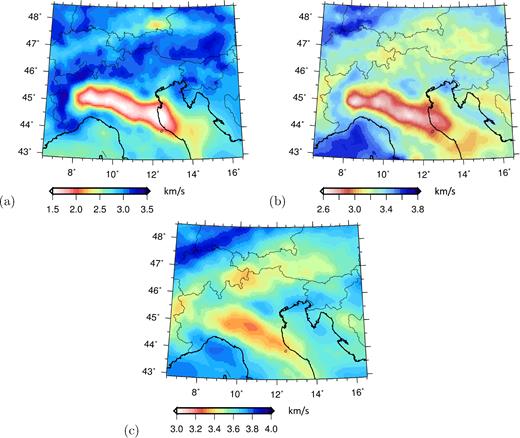
Rayleigh-wave phase-velocity maps of Kaestle et al. (2018), at periods of (a) 6 s, (b) 16 s and (c) 25 s.

Because the station distribution is non-uniform, the curve ∂S and, as a consequence, the vector n in eq. (34) are not uniquely defined. We avoid this difficulty by replacing eq. (34) with its far-field approximation (39), which can be implemented without specifying n. Preliminary experiments show that, despite the small size of the study region, the location of the backward propagating wave field’s focus is not visibly affected by this approximation. We plan to find ways to implement (34) exactly in future work, but we believe that the simplified approach employed here is adequate to the scope of this article. We accordingly time-reverse the traces, and propagate them backward in time, essentially implementing the right-hand side of eq. (45). Again, waves are propagated through the map of Fig. 1(b).

We obtain a pair of animations, one based on ray theory and the other on SPECFEM2D. Samples of both are shown in Fig. 2. Fig. 3 shows the prescribed and reconstructed signal at the known source location, again for both methods. While the backward propagating wave fields differ because of the mentioned physical differences in the implementation (excitation by initial displacement versus point force, curved membrane versus Mercator projection), it appears from Figs 2(c) and (d) that the maximum amplitude with respect to time and position in both simulations corresponds to the known, initial source location. This confirms the validity of surface-wave time reversal as a tool to localize/image a seismic source, despite the severe non-uniformity in receiver distribution. The maximum is less pronounced in the spectral-element simulation, resulting in normalized amplitudes throughout the simulation to be larger than ray-theory-based amplitudes. After focusing, in the absence of an ‘acoustic sink’ (Section 4.2), a non-physical wave field propagates away from the source. There are no major differences in the quality of focusing achieved by ray-theory versus SPECFEM2D backward-propagation.

Figure 2.

Snapshots of the ray-theory (left) and SPECFEM2D (right) synthetic-data time-reversal simulations (Section 6.1). Station locations are denoted by red triangles, the source location by a yellow circle. We define t = 0 as the time when the source experiences the maximum displacement according to the Ricker wavelet in the forward simulations; backward propagation starts at the time corresponding to the last data sample employed in our exercise, and time increments in time-reversal simulations are considered to be negative. For each of the two time-reversal simulations, amplitudes are normalized to the maximum value obtained in the simulation, corresponding to source location at t = 0. Snapshots (a) and (b) are taken at time t = 65 s; (c) and (d) at t = 0 s, (e) and (f) at t =−35 s. As explained in Section 6, ray-theory and SPECFEM2D wavefields can be compared only qualitatively. Snapshots (c) and (d) show that the time-reversed wavefield focuses at the ‘epicentre’ location.

Figure 3.

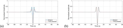
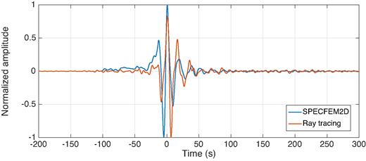
Synthetic test of Section 6.1. Normalized time-reversed and backward-propagated displacement (dashed red curves) computed at the known location of the source, via (a) SPECFEM2D and (b) ray theory. In both cases, the known source time function is shown (blue curve) for comparison. In panel (a), the difference between forcing term and reconstructed signal is explained by the fact that, in SPECFEM2D, displacement is initiated by prescribing a point force, rather than a displacement as in the ray-theory case.

6.2 Ambient-noise cross-correlations

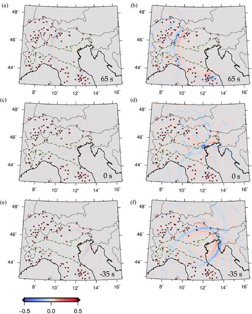
Cross-correlations of ambient signal form a perfectly suited data set to validate a source-localization method: each cross-correlation is an approximation for the corresponding receiver–receiver Green’s function, and the location of both receivers is naturally well known. We select station LSD.GU as our virtual ‘test’ source, and time-reverse and backward propagate ambient-noise based Green’s functions associated with it. (Noise cross-correlations will be described in a separate study (Molinari et al. in preparation, 2018).) This amounts to implementing the right-hand side of eq. (39) via our two algorithms. We first Butterworth-filter vertical-component cross-correlations around 16 s (low and high corner frequencies corresponding to periods of 26 and 6 s, respectively), and, as in Section 6.1, propagate time-reversed signal through the Rayleigh-wave phase-velocity map of Fig. 1(b). The results of this exercise are shown in Figs 4 and 5. Again, despite the poor azimuthal station coverage in this example, the time-reversed wave field focuses quite precisely on the virtual source, in both the ray-theory and SPECFEM2D implementations. In both cases, the maxima of the time-reversed wave field at the known source location are correctly achieved at t = 0. Similar to Section 6.1, non-physical signal naturally emerges after focusing.

Figure 4.

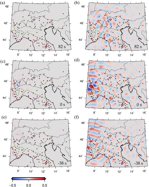
Snapshots of the ray-theory (left) and SPECFEM2D (right) time-reversal simulations of real noise cross-correlations described in Section 6.2, in the 6-to-26 s period band. This is similar to Fig. 2, but synthetic traces are replaced by cross-correlations of ambient data recorded at station LSD.GU (yellow circle) and all other stations whose locations are denoted by red triangles. Ambient-noise cross-correlations approximate the Green’s function for each station pair, and, in this exercise, station LSD.GU can accordingly be thought of as a ‘virtual source’. Snapshots (a) and (b) are taken at time t = 82 s; (c) and (d) at t = 0 s, (e) and (f) at t =−38. Snapshots (c) and (d) show that the time-reversed wave field indeed focuses at the location of station LSD.GU.

Figure 5.

Time-reversed and backward-propagated empirical, ambient-noise based Green’s functions (Section 6.2), computed at the location of the virtual source, that is, station LSD.GU, via SPECFEM2D (blue curve) and ray theory (red).

If station coverage were uniform and the noise-based Green’s functions perfectly reconstructed, the time-reversed signal at LSD.GU (Fig. 5) should closely approximate an impulse, which is not the case. We have seen, however, from the results of Section 6.1 and in particular Fig. 3, that the source time function can be reconstructed well even when the station coverage is poor. We infer that artefacts in the trace of Fig. 5 result from inaccuracies in the reconstructed Green’s function. This is not surprising because, while the phase of Green’s functions is reconstructed well by ambient-noise cross-correlation, their amplitude probably is not (e.g. Ekström et al.2009).

We next iterate the ray-theory procedure for the 4-to-10 s and 20-to-30 s period bands, and show the results in Figs 6 and 7. Membrane-wave propagation is modelled using phase-velocity maps at 6 and 25 s periods (Figs 1 a and c), respectively, again from Kaestle et al. (2018). The quality of focusing is comparable to the intermediate-period case (Fig. 4), and can be considered high, in view of the non-uniformity of station distribution. This result confirms that our algorithm can be applied to a variety of surface-wave modes, and, as far as reliable phase-velocity and Green’s function estimates are available, is fairly independent of period, and of the width of the passband.

Figure 6.

Snapshots of time-reversal simulations of real noise cross-correlations, in the 4-to-10 s (left) and 20-to-30 s (right) period bands. As in Fig. 4, cross-correlated data were recorded at station LSD.GU (yellow circle) and all other stations whose locations are denoted by red triangles. Snapshots were selected at the same times as in Fig. 4. Snapshots (c) and (d) show that, also in these period bands, the time-reversed wave field focuses at the location of station LSD.GU.

Figure 7.

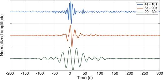
Same as Fig. 5, but traces obtained (via ray theory only) in the period bands 4-to-10 s (blue curve), 6-to-26 s (red) and 10-to-20 s (green) are shown.

6.3 Recordings of the Emilia earthquake of 2012 May 29

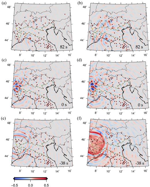
We apply our ray-theory- and SPECFEM2D-based algorithms to vertical-component recordings of the magnitude Mw=5.6 (MI=5.8) Emilia earthquake of 2012 May 29, 7:00:03 AM. These data, discussed in detail by Molinari et al. (2015), are shown here in Fig. 8. Traces are filtered around 16 s, the same way as in Section 6.2, before time reversal and backward propagation; propagation is modelled according to the 16s Rayleigh-wave phase velocity map of Fig. 1(b). Results are summarized in Figs 9 and 10. Early time-steps (e.g. Figs 9 a and b) are characterized by the emergence of time-reversed late arrivals, that we believe to be associated with reverberations, for example, at the sharp boundaries between Po plain and surrounding mountain ranges. This signal does not focus sharply anywhere on our membrane, and can accordingly be neglected in this context. Direct-arrival surface waves, on the other hand, do focus at the known epicentre location in both our implementations (Figs 9 c and d). Similar to Sections 6.1 and 6.2, non-physical signal again emerges after focusing (Figs 9 e and f).

Figure 8.

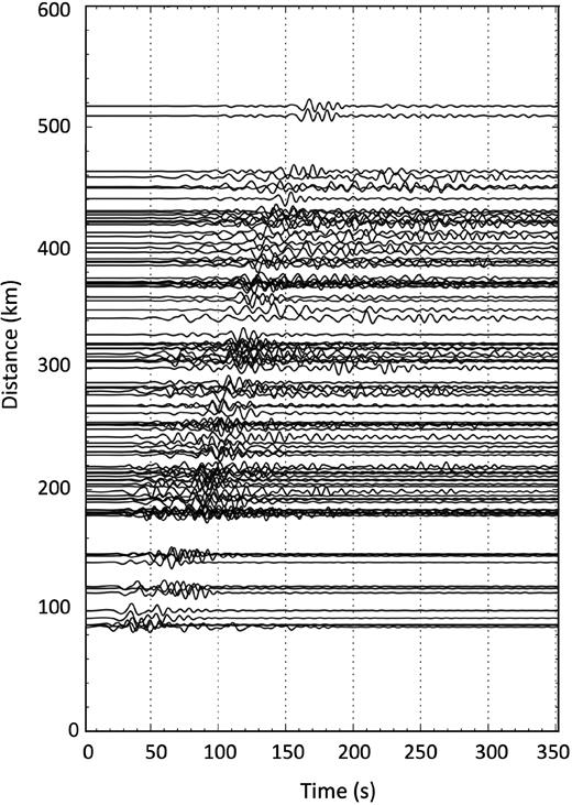
Normalized vertical-component recordings of the M_w = 5.6 (MI=5.8) Emilia earthquake of 2012 May 29 (e.g. Molinari et al.2015), that we time-reverse and backward-propagate as discussed in Section 6.3. The vertical axis corresponds to epicentral distance, and each trace is plotted about its associated epicentral distance. All traces are Butterworth-filtered around 16 s as described in Section 6.3.

Figure 9.

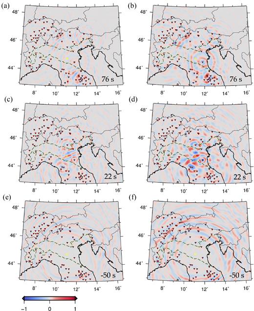
Snapshots of the ray-theory (left) and SPECFEM2D (right) time-reversal simulations of real earthquake data described in Section 6.3. Again, the locations of stations utilized in the time-reversal simulation are denoted by red triangles, while the earthquake epicentre is marked by a yellow circle. We define t = 0 as the earthquake origin time as reported by the Centro Nazionale Terremoti at INGV. Snapshots (a) and (b) are taken at time t = 76 s; (c) and (d) at t = 22 s, (e) and (f) at t = −50. Snapshots (c) and (d) show that the time-reversed wave field focuses at the epicentre of the earthquake.

Figure 10.

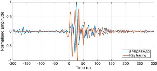
Time-reversed signal at the epicentre of the Emilia earthquake as reconstructed by SPECFEM2D (blue curve) and ray theory (red) time reversal. Again, we define t = 0 as the earthquake origin time; t should be interpreted as in Fig. 9, that is, negative t corresponds to time after focusing in a time-reversal simulation.

Fig. 10 shows that the maximum amplitude of the reconstructed vertical displacement at the epicentre occurs at t = 22s according to spectral-element time reversal; this delay with respect to the reported earthquake origin time is comparable with the considered surface-wave period, and, in order of magnitude, with typical discrepancies between body- and surface-wave-based estimates of rupture times. The ray-theory simulation results in multiple maxima between 0 and 50 s. All this presumably reflects the complexity of surface-wave generation at the source, as well as errors introduced by the mentioned, non-physical propagation of the time-reversed wave field after focusing.

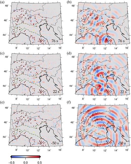
We repeat ray-theory time reversal in the 4-to-10 s and 20-to-30 s passbands, and show the results in Figs 11 and 12. Focusing of the time-reversed wave field is less sharp both in space and time (although, interestingly, in late snapshots of the time-reversal simulation (Figs 11 e and f), wave fronts are nicely centred on the earthquake epicentre). We ascribe the loss in source localization accuracy to the significant reduction in the width of the passbands, with respect to the previously discussed, 6-to-26 s simulation: we had anticipated in Section 1 that focusing of the time-reversed wave field is enhanced by combining as many time-reversed surface-wave modes as possible. In our future work, we plan to more rigorously take advantage of this effect, multiplication surface-wave potential and their horizontal gradients by the radial eigenfunctions U(ω), V(ω), W(ω) according to eqs (5) and (6), before integrating over the entire surface-wave frequency range.

Figure 11.

Snapshots of ray-theory time-reversal simulations of real earthquake data, in the 4-to-8 s (left) and 20-to-30 s (right) period bands. Snapshots were selected at the same times as in Fig. 9. All symbols are defined as in Fig. 9.

Figure 12.

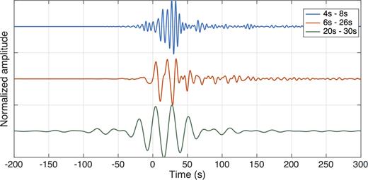
The ray-tracing based trace of Fig. 10 (red curve, 6-to-26s period band) is compared to analogous traces obtained for the 4-to-8s (blue) and 20-to-30s (green) bands. Each trace is normalized to its maximum.

Importantly, our analysis of time-reversed earthquake data shows that even at relatively short epicentral distances, where they are obscured by the body-wave coda, surface waves can still emerge in a time-reversal exercise. Focusing of the backward-propagated signal at the source can be thought of as a form of constructive interference. For time-reversed waves emitted at various station locations to interfere constructively, their backward propagation has to be modelled correctly. In our approach, time-reversed seismograms are filtered around one surface-wave frequency, and backward-propagated via the known Green’s function (i.e. phase-velocity map) for that frequency. In other words, only the propagation of time-reversed signal associated with surface waves at that frequency is modelled correctly, and it is only this signal that will contribute to ‘constructive interference’ and to focusing of the time-reversed wave field. Accordingly, circular wave fronts that can be associated with body-wave signal, and that do not focus at the epicentre (or elsewhere) are visible in Figs 9(a) and (b). We infer that surface-wave time reversal can indeed function as a source-imaging method also at relatively small epicentral distances, independently of how clearly surface waves can be identified visually on seismograms.

7 CONCLUSIONS

By taking advantage of the theory of surface-wave ‘potentials’, we have reduced the problem of surface-wave propagation to 2-D (‘membrane waves’). We have shown that 3-D wave fields can then be reconstructed from monochromatic 2-D ones, once radial surface-wave eigenfunctions (Section 2) are known; in this study, however, we only studied the propagation of surface-wave potentials in 2-D. We implemented a surface-wave time-reversal algorithm that can rely on either spectral-element or ray-theory models of wave propagation. In both cases, the theory is validated by application to real seismometer arrays in Central Europe. First, a synthetic test is implemented by computing approximately monochromatic membrane-wave seismograms at all receiver positions, from an arbitrary selected source location in Northern Italy. In a second experiment, synthetic traces are replaced by approximate Green’s functions, obtained by cross-correlating the real ambient signal recorded at one station of the array with that recorded at all other stations. Finally, waveforms from a magnitude-5.6 event in the Po plain are used. In all three cases, time reversal and backward propagation of the data result in focusing of the signal at the location and time of the source, despite the severe non-uniformity of data coverage, inaccuracies in ambient-noise-based Green’s function reconstruction, and difficulties in disentangling surface-wave signal from the body-wave coda. Importantly, our experiment described in Section 6.3 suggests that time reversal and backward propagation using the surface-wave Green’s function result in focusing of surface waves at the epicentre even at distances less than teleseismic, where surface waves carry less energy than body waves and their coda. These results encourage further applications of our method, in particular to the task of mapping, in space and time, rupture processes associated with large earthquakes.

ACKNOWLEDGEMENTS

We are indebted to Julien de Rosny, Jean-Paul Montagner, Daniel Peter, Piero Poli and Kees Wapenaar for their insightful advice, and to the editor Michael Ritzwoller for having handled our manuscript. Emanuel Kaestle provided his phase-velocity maps while Piero Poli shared his ambient-noise cross-correlations. Several figures were created with the Generic Mapping Tools software (Wessel & Smith 1991), and we made wide use of the ObsPy software (Krischer et al.2015). LB and MR are supported by the European Union’s Horizon 2020 research and innovation programme under the Marie Sklodowska-Curie grant agreement 641943 (WAVES network). IM is supported by the Swiss National Science Foundation SINERGIA Project CRSII2-154434/1 (Swiss-AlpArray).

APPENDIX A: DIPOLE SOURCES

The term ‘dipole source’ refers here to the superposition of two impulsive point sources of opposite sign, located at two different points separated by a very small distance d. In this study, the concept of dipole emerges from the physical interpretation (Section 4.2) of eq. (34), relating the time-reversed, backward propagating wave field to the signals initially recorded by a receiver array. In the general context of wave physics, dipole sources are used, for example, to formulate a modern, ‘corrected’ version of Huygens’ principle (Baker & Copson 1950; Miller 1991).

The mathematical expression for a dipole source can be obtained by first writing the forcing term q defined in Section 3 as the sum of two equal source distributions f(x, ω) shifted in space by the vector d (of magnitude d) and switched in sign one with respect to the other, that is,

\begin{equation*} q({\bf x},\omega )=f\left({\bf x}+{\bf d}\right)-f({\bf x}). \end{equation*}

(A1)

A first-order Taylor expansion around the point x_S then gives

\begin{equation*} f\left({\bf x}+ {\bf d}\right) \approx f({\bf x}) + {\bf d} \cdot \nabla _1 f({\bf x},{\bf x}_S). \end{equation*}

(A2)

Substituting expression (A2) into expression (A1), we find

\begin{equation*} q({\bf x},\omega ) \approx {\bf d} \cdot \nabla _1 f({\bf x},{\bf x}_S). \end{equation*}

(A3)

Finally, the sought expression is found by replacing f with a Dirac δ(x − x_S); since q accordingly becomes infinitely large at x_S and zero elsewhere, the magnitude of d ceases to have meaning and d can be replaced by the corresponding unit vector |${\hat{\bf d}}$|⁠, so that

\begin{equation*} q({\bf x},\omega )={\hat{\bf d}} \cdot \nabla _1 \delta ({\bf x}-{\bf x}_S) \end{equation*}

(A4)

(e.g. Wapenaar & Berkhout 1989,section I.3.1).

Let us next find a simple expression for the response of a medium to dipole forcing. Recall that we have introduced the Green’s function |$\mathscr {G}_{\text{2D}}({\bf x},{\bf x}_S,\omega )$| in Section 3 as the solution of eq. (23) with q(x, ω) =δ(x − x_S), that is,

\begin{equation*} \nabla _1^2 \mathscr {G}_{\text{2D}}({\bf x},{\bf x}_S,\omega ) + \frac{\omega ^2}{c^2} \mathscr {G}_{\text{2D}}({\bf x},{\bf x}_S,\omega ) = -\rm{\small I}\omega \delta ({\bf x}-{\bf x}_S). \end{equation*}

(A5)

Applying the operator |${\hat{\bf d}} \cdot \nabla _1$| to both sides of eq. (A5) yields

\begin{equation*} \nabla _1^2 \left[{\hat{\bf d}} \cdot \nabla _1 \mathscr {G}_{\text{2D}}({\bf x},{\bf x}_S,\omega ) \right] + \frac{\omega ^2}{c^2} \, {\hat{\bf d}} \cdot \nabla _1 \mathscr {G}_{\text{2D}}({\bf x},{\bf x}_S,\omega ) = -\rm{\small I}\omega \, {\hat{\bf d}} \cdot \nabla _1 \delta ({\bf x}-{\bf x}_S). \end{equation*}

(A6)

We infer from eq. (A6) that the solution of eq. (23) with q(x, ω) = |${\hat{\bf d}} \cdot \nabla _1 \delta ({\bf x}-{\bf x}_S)$| is simply |${\hat{\bf d}} \cdot \nabla _1 \mathscr {G}_{\text{2D}}({\bf x},{\bf x}_S,\omega )$|⁠.

Alternatively, Boschi & Weemstra (2015, eqs E1–E3) define the Green’s function G_2D in the time domain as the solution of

\begin{equation*} \nabla ^2 G_{\text{2D}} - \frac{1}{c^2} \frac{\partial ^2 G_{\text{2D}}}{\partial t^2} = 0 \end{equation*}

(A7)

with initial conditions

\begin{equation*} G_{\text{2D}}({\bf x},{\bf x}_S,0) = 0, \end{equation*}

(A8)

\begin{equation*} \frac{\partial G_{\text{2D}}}{\partial t} ({\bf x},{\bf x}_S,0) = \delta ({\bf x}-{\bf x}_S). \end{equation*}

(A9)

Applying, again, |${\hat{\bf d}} \cdot \nabla _1$| to both sides of eqs (A7)–(A9), we find that |${\hat{\bf d}} \cdot \nabla _1 G_{\text{2D}}({\bf x},{\bf x}_S,t)$| is the field resulting from a dipole initial velocity at x_S. This, or rather its Fourier transform |${\hat{\bf d}} \cdot \nabla _1 G_{\text{2D}}({\bf x},{\bf x}_S,\omega )$|⁠, is what we call ‘dipole response’ throughout this study.