


Abstract
The simulation of product behavior is a vital part of current virtual product development. It can be expected that soon there will be more product simulations due to the availability of easy-to-use finite element analysis software and computational power. Consequently, the amount of accessible new simulation data adds up to the already existing amount. However, even when using easy-to-use finite element software tools, errors can occur during the setup of finite element simulations, and users should be warned about certain mistakes by automatic algorithms. To use the vast amount of available finite element simulations for a data-driven finite element support tool, in this paper, a methodology will be presented to transform different finite element simulations to unified matrices. The procedure is based on the projection of nodes onto a detector sphere, which is converted into a matrix in the next step. The generated matrices represent the simulation and can be described as the DNA of a finite element simulation. They can be used as an input for any machine learning model, such as convolutional neural networks. The essential steps of preprocessing the data and an application with a large dataset are part of this contribution. The trained network can then be used for an automatic plausibility check for new simulations, based on the previous simulation data from the past. This can result in a tool for automatic plausibility checks and can be the backbone for a feedback system for less experienced users.
Method for plausibility checks of finite element simulations.
Conversion of finite element analysis into a readable format for neural networks.
Application of convolutional neural networks on finite element analysis.
1. Introduction
Modern technology enables us to capture and store vast quantities of data, but the main challenge is to turn data into information and information into knowledge (Witten, Hall, Frank, & Pal, 2017). Many organizations realize that survival is only possible by exploiting available data intelligently (Van der Aalst, 2014). Furthermore, the available data are increasing faster than ever before in history (Smolan & Erwitt, 2012), and methods for the imputation of missing data are available (Meechai, Tongsima, & Chan, 2016). In product development, a huge source of data is the simulation of product behavior. These simulations are a vital part of the development process (Spruegel, Schroeppel, & Wartzack, 2017), and various tools can be applied to simulate the later product behavior: multibody simulation, modal analysis, manufacturing simulation, fluid simulation, or structural mechanic finite element (FE) simulation. This is state of the art, and most companies perform numerical simulations. Often, the results are only used for the design and validation process of one specific product or part. The data will be stored afterward only on the legal duty of proof, but will not be processed for any other purpose. However, a massive amount of knowledge is included in these datasets, such as the reduction of the real load case to a numerically solvable problem or unique material data. In today's industry, this information is lost because the huge amount of simulation data cannot be investigated automatically.
Furthermore, these data could be used for applications such as plausibility checks of new simulations or to maintain knowledge in companies even when personnel changes. Plausibility checks are a method to check the simulation results whether the calculated values are plausible for the given load case or not. Especially employees with less knowledge in this area or with a specific component can benefit significantly from this type of examination.
Several procedures are necessary to apply plausibility checks in FE simulations. One important part is the data labeling for supervised learning (Sixt, Wild, & Landgraf, 2018), and even more mandatory for the execution of the method is the transformation of the heterogeneous simulation data to a fixed form of numerical values. These values can then be used as input for convolutional neural networks (CNNs). Some methods for 3D object classification exist to transfer geometry data to machine learning algorithms: RS-CNN (Liu, Fan, Xiang & Pan 2019), Point2Sequence (Liu, Han, Liu & Zwicker, 2019), binVoxNetPlus (Ma, An, Lei, & Guo, 2019), PANORAMA-ENN (Sfikas, Pratikakis, & Theoharis, 2018), VoxNet (Maturana & Scherer, 2015) or DeepPano (Shi, Bai, Zhou, & Bai, 2015). However, all of these mentioned models apply different methods to a point cloud to predict the corresponding geometry model. However, these various techniques only use the geometry of the individual points and geometrical properties derived from them, such as normal directions or images.
In contrast to that, this new approach is capable of using FE simulations as input. The simulation data also contain the geometry of the part, but more information regarding boundary conditions and calculated results. This novel approach uses all the data necessary for and all the data generated by an FE simulation to make the simulation more accessible and readable for neural networks. The idea of this new procedure model is to classify both inputs and outputs of simulations according to prespecified labels. This leads to the advantage that obviously false simulations can be automatically identified. Deep learning can eliminate the need for further feature engineering and is therefore used in this paper. A CNN is used for the classification task because it combines the benefits of neural networks, the processing of large amounts of data, and the ability to process large matrices. Every other machine learning algorithm is also suitable for this problem, as the stated method is a data preprocessing procedure, which generates a uniform input matrix.
In the following, a methodology for automatic plausibility checks is demonstrated, which is described in detail after the preliminaries. Numerical finite element simulations are classified as either plausible simulations (likely valid) or non-plausible simulations (very likely to contain errors and wrong results). Subsequently, the database, the CNN architecture, and the classification accuracy of the trained network are shown.
2. Preliminaries
For numerous applications in architecture, computer vision, or robotics, it is necessary to transfer geometry data to machine learning algorithms. In general, a differentiation is established between the task and the type of input data (Xu, Kim, Huang, & Kalogerakis, 2017). The goal of transforming geometry data to machine learning algorithms can be the segmentation of the shape into smaller patches, the classification of a specific part, the retrieval of similar objects, or the matching of different point clouds into one. Examples for other 3D data input are numerical simulation data (Duesing, Sadiki, & Janicka, 2006), scan data from optical (Bosche & Haas, 2008) and tactile measuring techniques (Aldoma et al., 2011), similarity recognition with computer-aided design (CAD) models (Zehtaban, Elazhary, & Roller, 2016), different geographical (Verschoof & Lambers, 2019), airborne (Antonarakis, Richards, & Brasington, 2008) and vehicle (Ogawa, Sakai, & Suzuki, 2011) LiDAR images, and magnetic fields and images from coronal diagnostic spectrometer (Ireland, Walsh, & Galsgaard, 1998).
A large amount of such data already illustrates the need to transfer these data to machine learning algorithms for multiple reasons. For the transfer of such data to the previously described algorithms, several methods are already available. As the effectiveness of new techniques is usually shown with an application to a dataset, each new method needs a certain amount of data. Based on the four tasks mentioned above, the stated method in this paper can best be sorted in the shape classification. Many of these methods use the Princeton ModelNet10 or ModelNet40 dataset (Wu et al., 2015) to classify a large amount of 3D shapes in 10 or 40 categories. Currently, the three methods with the highest classification accuracy for the ModelNet40 dataset are HGNN with 96.6% (Feng, You, Zhang, Ji, & Gao, 2019), iMHL with 97.16% (Zhang, Lin, Zhao, Ji, & Gao, 2018), and RotationNet with 97.37% (Kanezaki, Matsushita, & Nishida, 2018). These methods are especially good in the data preparation and the given classification task. Broader approaches that are applicable for multiple use cases with point clouds are PointNet (Qi, Su, Mo, & Guibas, 2017) and PointNet++ (Qi, Yi, Su, & Guibas, 2017). In contrast to 3D shape classification, the method stated in this paper can transform additional information. This ability should be demonstrated by its application to FE simulations.
2.1. Available data from finite element analysis
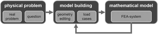
Finite element analysis (FEA) is a standard method in modern product development processes (see simulation-driven design; Tatipala, Suddapalli, Pilthammar, Sigvant, & Johansson, 2017). In general, the task of an FE analysis is to transfer a real existing problem into a mathematical model. Figure 1 shows an overview of the model building process in FE analysis. This generated virtual model can then be used for drawing conclusions about reality. The starting point is the physical problem, which consists of the real problem and the associated questions. From this physical problem, a model is derived, which contains the geometry and load cases. Simplifications have to be assumed in the modeling phase, such as approximation of geometry and physical parameters, neglect of molecular structure, or simplification of material behavior.
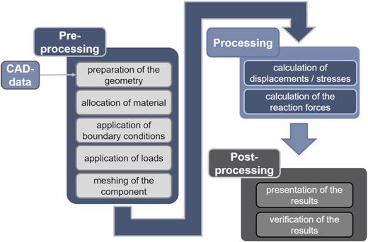
Typically the FEA is divided into three sequential steps, which are preprocessing, solving, and postprocessing, as shown in Fig. 2 (Vajna et al., 2018). During the preprocessing several input information must be specified, such as the geometry (in most cases, CAD models are used), material properties (Young's modulus, shear modulus, yield strength, etc.), boundary conditions (supports, displacements, etc.), and loads (forces, moments, pressures, pretensions, etc.). If assemblies are simulated, also the contacts need to be defined. Often the geometry must be prepared because not all details are necessary or essential for the structural analysis. During the preprocessing, also the FE mesh (discretized representation of the geometry) is generated. After the solving/processing step, the results of the FE simulation can be used in the postprocessing step. Typical results of a structural mechanic FEA are safety factors, deformations, stresses, surface pressures, or reaction forces. These results are node-bound to the FE mesh; this means that for each node of the FE mesh, the stresses or deformations in different directions are available after the simulation. Since FE analysis is often the basis for severe decisions and thus has a significant influence on costs, methods for controlling the results have been developed. Examples are the application of simple analytical models, calculation of FE models with different complexity, comparison of results with analytical solutions, or validation by testing (Vajna et al., 2018).
2.2. Neural networks
Neural networks are applied in many fields of today's research, such as modeling new mechanical processes like deep drawing-extrusion (Ashhab, Breitsprecher, & Wartzack, 2014), challenging gender determination task from CT-scan images of human crania (Trentin, Lusnig, & Cavalli, 2018), segmentation of CT images using CNNs (Vania, Mureja & Lee, 2019), learning to calculate the heat transfer for 2D geometries (Edalatifar, Tavakoli, Ghalambaz, & Farbod, 2020), or understanding the dynamic folding process and predicting its dynamic behaviors of origami structures (Liu, Fang, & Xu, 2019).
Data preprocessing plays an important role before neural networks can be trained to perform regression or classification on the data (Famili, Shen, Weber, & Simoudis, 1997). This includes data reduction and data normalization (Bishop, 1996). Especially deep learning algorithms try to discover useful representations of the data defined in terms of lower level features (Bengio, 2012). Graphics processing units (GPU) excel at fast matrix and vector multiplications and are therefore very well suited for the training of neural networks (Schmidhuber, 2015) and these features.
Even though current CNNs have some disadvantages (e.g. the need for large amounts of training data or high computational cost; Van Doorn, 2014), they can be used for the classification of large, multidimensional input matrices with many numeric input values effectively.
3. Methodology
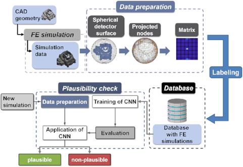
The whole process of classifying an FE simulation is depicted in Fig. 3. The process starts with the simulation itself and ends with a defined label for a new simulation, whether the results are plausible or not.
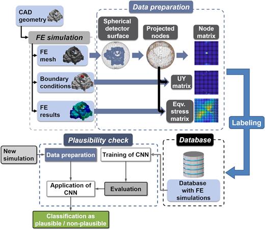
Overview of the entire plausibility check procedure.
To classify new simulations based on their results, a database must first be established, which serves as a foundation for training the neural network. The calculated results are then used for generating the input data for the CNN. In order to generate a sufficient amount of data, many parameter studies must be carried out and afterward prepared. In addition to the pure generation of the data, these must also be labeled accordingly so that a subsequent classification is possible. Each of the different steps in the procedure is explained in detail in the following.
The overall aim is to generate a detector matrix with 36 × 36 pixels from nodal simulation input; any other source of 3D Cartesian coordinates is possible as well. The number of pixels can also be changed with the same methodology. The more pixels the detector sphere has, the more precise is the representation of the simulation data and the geometry of the considered part. The size of the input for the neural network increases in size with more pixels. The basic idea of the method is to generate detector pixels of the same surface area on a spherical surface, which is located around the part or point cloud.
Figure 4a shows the detector surface and a very simple meshed part inside the detector sphere. The mesh is generated during the FEA and is stored as a matrix in Cartesian coordinates together with the node numbers. The center of gravity of the point cloud of the FE nodes is the same as the center of the detector surface. The orientation of the part can be unified by principal component analysis (PCA). A detailed explanation of the application of this analysis can be found in Spruegel et al. (2018). Other methods, such as the standardized orientation of bounding boxes of the parts, are also possible. All nodes are projected onto the surface of the sphere (Fig. 4b).
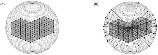
Exemplary representation of the spherical detector surface with a meshed part.
Angle ϴ for detector sphere with 36 × 36 pixels.
| Segment 1 | |${{\rm{\Theta }}_n}$| | |${{\rm{\Theta }}_{n + 1}}$| | |${{\rm{\Theta }}_{n + 1}} - {{\rm{\Theta }}_n}$| |
|---|---|---|---|
| Pixel 1 | 0° | 19.1881° | 19.1181° |
| Pixel 2 | 19.1881° | 27.2660° | 8.0779° |
| Pixel 3 | 27.2660° | 33.5573° | 6.2913° |
| … | … | … | … |
| Pixel 17 | 83.6206° | 86.8153° | 3.1946° |
| Pixel 18 | 86.8153° | 90° | 3.1847° |
| … | … | … | … |
| Pixel 35 | 152.7339° | 160.8119° | 8.0779° |
| Pixel 36 | 160.8119° | 180° | 19.1881° |
In Fig. 5, the different angles ϴ are shown on the detector surface. Furthermore, the area of the corresponding pixel is displayed.
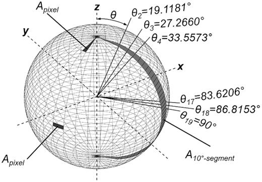
Segments of the sphere and corresponding angles.
At each pixel, the number of projected nodes can be monitored. In Fig. 6a, the projected surface of the detector sphere is shown together with the number of projected nodes at each pixel. The projection can be converted to a numerical matrix of 36 × 36, which includes the number of projected nodes in each pixel (see Fig. 6b).
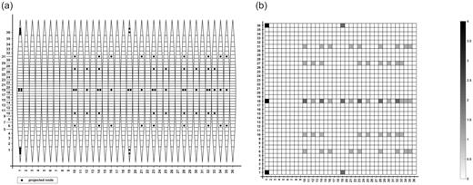
Generation of detector matrix from the spherical surface.
In FEA, all the relevant information is nodal bound; therefore, the described methodology can be used to generate matrices for all the needed FE information, such as boundary conditions, loads, or the results from the simulation. If meshed structures are applied with boundary conditions, the resulting displacements can be calculated. With Hooke's law, the stresses at each corner node of each element can be calculated as well. Figure 7 illustrates the equivalent (von Mises) stress in MPa of a cross-section of the L-shaped block. Besides the corner nodes also the intermediate nodes of each of the eight elements are shown. All the equivalent stress values of the block are projected to a 2D detector sphere, and the sum of the stresses can be calculated.
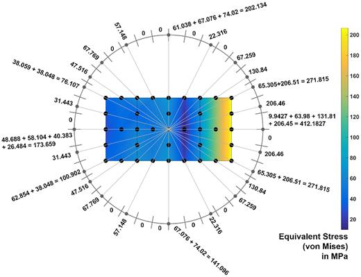
Projection of equivalent (von Mises) stress onto the detector sphere (here: 2D example).
Currently, the methodology uses one matrix for each of the following 20 FE simulation inputs and outputs: mesh (1), fixed displacements in x-, y-, and z-direction (3), fixed rotation in x-, y-, and z-direction (3), applied positive forces in x-, y-, and z-direction (3), applied negative forces in x-, y-, and z-direction (3), positive deformations in x-, y-, and z-direction (3), negative deformations in x-, y-, and z-direction (3), and equivalent stress (1). All these matrices with a fixed size of 36 × 36 can be combined into a large matrix with the size 36 × 720. This assembled matrix is called the DNA of an FE simulation as it contains all relevant information about the simulation.
4. Application
In this chapter, the previously presented methods are demonstrated in more detail. First, the data basis is explained and the different simulation models are presented. Then, the parameters for the data preparation and normalization of the results are pointed out. The training parameters for the different CNN architectures are also part of the chapter, as well as the listing of the results and presentation of the effects of different CNN layouts.
4.1. Database
In industry, a broad pool of FE simulations is usually available. Some suppliers of the automotive sector perform several thousand FE simulations a day. For the illustration of the whole process, a simulation database is generated with multiple geometries and different load cases for the individual parts. At first, the geometries are modeled as parametric CAD models. These models vary in shape according to specified geometry parameters. The database consists of three very different parts; each part can be modified in geometry by the specified parameters. The first part type is a wheel frame of an inline skate, the second part type is a mountain bike linkage plate, and the third part type is a six-cylinder crankshaft from an automotive combustion engine. The three different types of parts are shown in Fig. 8; each of these parts can be slightly modified regarding the geometry. The components were selected in a way that many basic shapes are represented. In this case, the database includes long, rotatory components, flat parts, and rather voluminous, cubic shapes. In Fig. 8, the minimal dimensions of each piece are shown in blue, and the maximum dimensions in transparent gray.
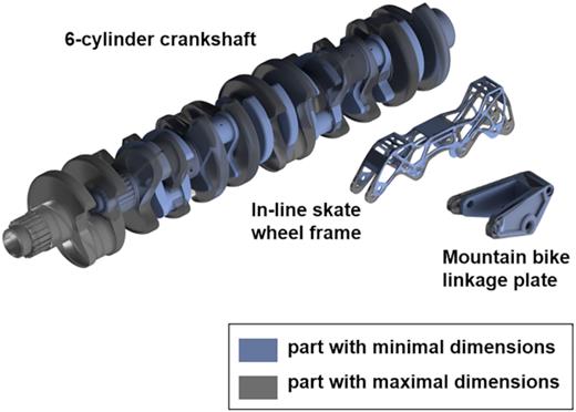
Part variations within the dataset.
Both the geometry dimensions and the applied forces, and the constant mesh size (10-node tetrahedral elements) for the FE mesh generator of the parts are sampled using D-optimal DoE (Design of Experiments) methods (Murray-Smith, 2015). The combination of DoE input parameters and parametric CAD models enables the buildup of extensive simulation studies. The different parameters and simulation model setups can be found in detail in Appendix 1.
The D-optimal DoE is performed twice, first for the combined training and validation data, and for a second testing dataset (Pareto split with 80:20). The first dataset is then separated randomly in training and validation dataset with a ratio of 90:10. Therefore, the overall ratio between training, testing, and validation is 72:20:8.
The finite element simulations are performed with ANSYS workbench, and the results are exported as text files during the postprocessing step of each simulation. The number of available data samples and the amount of raw simulation data are shown in Tables 2 and 3. These data are used to generate the DNA for each of the simulations, previously mentioned in Section 3.
Available finite element simulations.
| Part type | Training samples | Testing samples | Validation samples |
|---|---|---|---|
| Wheel frame | 6912 | 1920 | 768 |
| Linkage plate | 16 632 | 4200 | 1848 |
| Crankshaft | 7776 | 2160 | 864 |
| ∑ | 31 320 | 8280 | 3480 |
| Part type | Training samples | Testing samples | Validation samples |
|---|---|---|---|
| Wheel frame | 6912 | 1920 | 768 |
| Linkage plate | 16 632 | 4200 | 1848 |
| Crankshaft | 7776 | 2160 | 864 |
| ∑ | 31 320 | 8280 | 3480 |
Available raw simulation data in terabyte (TB).
| Part type | Training samples (TB) | Testing samples (TB) | Validation samples (TB) |
|---|---|---|---|
| Wheel frame | 1.080 | 0.410 | 0.120 |
| Linkage plate | 2.009 | 0.558 | 0.224 |
| Crankshaft | 6.210 | 1690 | 0.690 |
| ∑ | 9.299 | 2.658 | 1.034 |
| Part type | Training samples (TB) | Testing samples (TB) | Validation samples (TB) |
|---|---|---|---|
| Wheel frame | 1.080 | 0.410 | 0.120 |
| Linkage plate | 2.009 | 0.558 | 0.224 |
| Crankshaft | 6.210 | 1690 | 0.690 |
| ∑ | 9.299 | 2.658 | 1.034 |
4.2. Data preparation and application
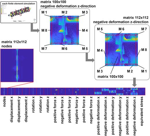
In Fig. 9, the generated DNA of one FE simulation of the crankshaft is shown. At first, 20 matrices with a size of 100 × 100 pixels are obtained. Such a matrix is shown for the negative deformation in the z-direction. In this matrix, one point in the upper left corner has no connection to the lower left or lower right corner, even so, these pixels are directly connected on the surface of the detector sphere. Therefore, 6 pixels on each side are projected to the other side of the matrix (these parts are labeled as “M1” to “M8” in Fig. 9). The result of these projections is a matrix with 112 × 112 entries, which can be derived for all 20 matrices. If these matrices are combined, as shown in the figure, the DNA of the FE simulation is generated, which has 20 matrices of 112 × 112 numeric values each.
Part variations within the dataset.
Each of these 20 matrices is different in the range of the individual values, and therefore needs normalization to archive typical input values for CNNs in the range from 0 to 1 (depending on the used deep learning framework).
Two different normalization strategies are applied to the data.
Strategy 1: each of the 20 matrices is divided by its maximum (for positive value matrices) or minimum (for negative value matrices).
Strategy 2: each of the matrices is normalized with an individual normalization strategy with additional knowledge from the finite element simulations:
node matrix: divided by a constant value of 10 000
displacement and rotation matrices: divided by the individual maximum of each matrix (similar to strategy 1)
force matrices: divided factor S1
deformation matrices: divided factor S2
equivalent stress matrix: divided factor S3
The constant value for the node matrix is chosen so that even very finely meshed components can be considered in the investigation. It is because by this value, theoretically 100 000 000 (matrix size 100 × 100) points can still be mapped by the projection method.
Factor S1 is defined by the ultimate tensile strength of the material Rm and the maximum dimensions of the finite element mesh in Cartesian x-, y-, and z-direction (xdim, ydim, and zdim). It is based on the maximum acceptable pressure load, and the constant factor of 800 has proven to be most appropriate in the investigations.
The second factor S2 is composed of the maximum dimension of the component in one direction and a fixed value. This value results from the reason that FE simulations usually show small displacements. Therefore, the value is chosen so that as many simulations as possible can be considered, in this case, up to a displacement of 5% related to the maximum component length.
As usual, an extensive amount of work lies in the correct labeling of the datasets, which defines the later applications. Besides plausibility checks, labels such as correct/incorrect or safe part design/part design near the load limit/unsafe part design could be used as other examples. The idea behind plausibility checks is to classify plausible simulations (likely valid) and non-plausible simulations (very likely to contain errors and wrong results) automatically. The used database contains two different labels for plausible and non-plausible datasets. Non-plausible simulations contain obvious errors, which an experienced simulation engineer would be able to identify. These incorrect results can have various causes. One source identified by the plausibility check is a global stress peak caused by a too coarse mesh. Furthermore, unrealistic tensions and deformations can be detected, which often results from incorrect load parameters or material data. Also, the user himself can bring errors into an FE simulation, resulting from a faulty model setup or wrongly entered load parameters.
The different datasets for training, validation, and testing of the CNNs are balanced and contain slightly more plausible simulations. The individual percentages are shown in Table 4.
Available finite element simulations.
| Plausible | Non-plausible | ∑Plausible & non-plausible | |
|---|---|---|---|
| Training | 17 519 (55.94%) | 13 801 (44.06%) | 31 320 (100%) |
| Validation | 1947 (55.95%) | 1533 (44.05%) | 3480 (100%) |
| Testing | 4645 (56.10%) | 3635 (43.90%) | 8280 (100%) |
| ∑Train & val & test | 24 111 (55.97%) | 18 969 (44.03%) | 43 080 (100%) |
4.3. Model training
After generating the different DNAs for each finite element simulation, various convolutional neural networks are trained, and the results are compared in Section 4.4. The overall aim is to demonstrate the novel approach to handle arbitrary finite element simulations to machine learning algorithms—especially neural networks. This enables deep neural networks to perform plausibility checks for new finite element simulations with the knowledge from previous simulations of different parts—this is one possible application, but many more are imaginable.
The basic CNN architecture is a VGG16 network, as published by Simonyan and Zisserman (2014). The network is adapted to a smaller image size of 100 × 100 and 112 × 112. Due to the smaller input size, the 5th convolution sequence group is no more necessary, as the input image can be reduced to 7 × 7 images after the 4th convolution layer sequence. The number of input channels is increased from 3-channel RGB input to 20-channel input for the described simulation dataset. For faster and more feasible training on a Tesla K40 GPU, the number of filters in the first sequence of convolution layers is 8 instead of 32 from the original VGG16 network. The number of filters is doubled in each new sequence of convolution layers. In Fig. 10, the network is shown for the training of the extended matrices (112 × 112 pixels). The network architecture for the 100 × 100 matrices has a smaller input layer; instead of 112 × 112 × 20, the input layer uses 100 × 100 × 20.
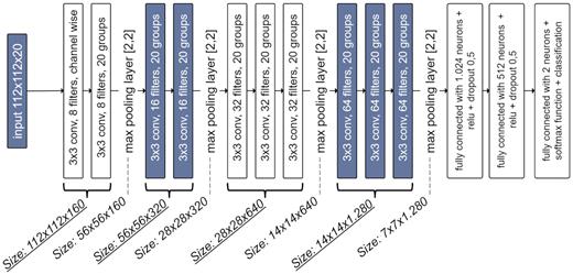
Adapted CNN architecture from VGG16 with a reduced number of convolution filters due to 20-channel input images.
In Table 5, the four different networks are listed with the corresponding matrix size and the used normalization strategy. The used deep learning framework is the MATLAB Deep Learning Toolbox R2019a, and a Tesla K40c is used for the training of the networks. The separate validation dataset is used to monitor the risk of overfitting to the training data. The performance of each trained network is evaluated with a separate testing dataset.
The four different CNNs and their parameters.
| Matrix size | Normalization | |
|---|---|---|
| CNN #1 | 100 × 100 | Strategy 1 |
| CNN #2 | 100 × 100 | Strategy 2 |
| CNN #3 | 112 × 112 | Strategy 1 |
| CNN #4 | 112 × 112 | Strategy 2 |
| Matrix size | Normalization | |
|---|---|---|
| CNN #1 | 100 × 100 | Strategy 1 |
| CNN #2 | 100 × 100 | Strategy 2 |
| CNN #3 | 112 × 112 | Strategy 1 |
| CNN #4 | 112 × 112 | Strategy 2 |
The different training options (mini-batch size, epochs, and iterations/epoch) are shown in Table 6, as well as the training time for 50 epochs. The batch size varies for the different projection resolutions due to hardware limitations; for the matrices with higher resolution, the limitation of the GPU is a mini-batch size of 200, and for the 100 × 100 matrices, the limit is 256. The solver for the training is an Adam optimizer, and an adaptive learn rate is used. The initial learn rate is 0.001, and the learn rate is reduced after every five epochs by a multiplicative factor of 0.1. Networks CNN #1, CNN #2, and CNN #3 use the Glorot weights and bias initializer (also known as Xavier initializer) for the convolution and fully connected layers. Due to insufficient learning behavior of CNN #4 with 112 × 112 matrices and normalization Strategy 2, another approach is used for this network. Instead of initializing the weights with Glorot, the trained weights and bias values of all convolution layers from CNN #3 after epoch 50 are used as initial weights and bias values for all convolution layers before the training of CNN #4.
Training options for the CNN architecture.
| 100 × 100 matrices | 112 × 112 matrices | |
|---|---|---|
| Mini-batch size | 256 | 200 |
| Training time | ≈ 2960 min | ≈ 4200 min |
| Iterations/epoch | 122 | 156 |
| Epochs | 50 | 50 |
| Initial learn rate | 0.001 (decreasing) | 0.001 (decreasing) |
| beta 1 (gradient decay rate) | 0.9 | 0.9 |
| beta 2 (decay rate of squared gradient moving average) | 0.99 | 0.99 |
In Fig. 11, the different training processes are shown. The training and validation accuracy is evaluated after each epoch. The validation accuracy is evaluated during the training process, but the testing accuracy is calculated after the 50th epoch. Checkpoints from the CNN during the training are used for this purpose after each epoch.
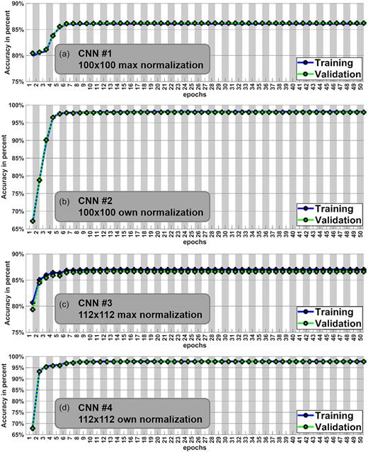
Training process of the four trained CNNs with the evaluation of the accuracies.
For the training process, a predefined epoch value of 50 was set for all different CNN variations, as can be seen in Table 6. Early stopping was not considered in this study because all nets should be trained under the closest possible conditions. However, Fig. 12 shows a section of the training process for the first 10 epoch steps for better visibility. The first graph displays the training accuracy for the different CNN versions, whereas the second graph illustrates the validation accuracy.

The training process of the four trained CNNs with the evaluation of the training and validation accuracies for the first 10 epochs.
TP: true positives
TN: true negatives
FP: false positives
FN: false negatives
4.4. Results and evaluation
The different training process evaluations from CNN #1, CNN #2, CNN #3, and CNN #4 (shown in Figs 11 and 12) show promising results without indications of overfitting. It is obvious that CNN #1 and CNN #3 achieve lower accuracies below 90%, whereas CNN #2 and CNN #4 with normalization Strategy 2 result in accuracies near 100%.
Especially the normalization strategy shows a significant impact on the performance of the trained networks. Consequently, the normalization Strategy 2 from Section 4.2 should be used for further investigations. The extended matrices do not lead to clearly better results; nevertheless, slight improvements from the extended matrices over the 100 × 100 matrices can be observed. If simulations of parts in different spatial orientations should be combined and used for the training, the extended matrices will probably perform a lot better than the standard matrices without extended margins. If the orientations from the finite element simulations are well known, there is no need to extend the matrices to 112 × 112, assuming that the classification task is to identify simulations that contain errors (plausibility checks).
Figure 13 shows the testing and validation accuracies for each of the four CNNs after the 50th epoch of the training process. The highest accuracy from the validation dataset and the testing dataset achieves CNN #2. A testing accuracy of 99.21% and a validation accuracy of 97.96% indicate a very well-trained network for the task of plausibility checks.
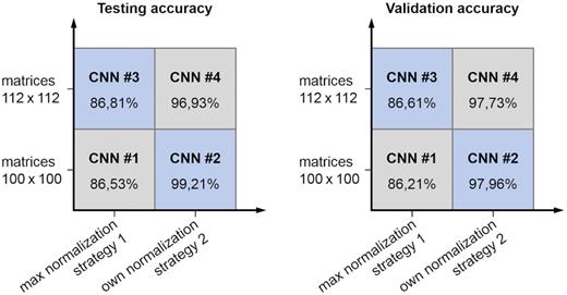
Testing and validation accuracy of the trained CNNs for different normalization strategies and matrix sizes.
5. Discussion
The described methodology with spherical detector surfaces can transfer inputs and outputs from finite element simulation to machine learning algorithms (i.e. convolutional neural networks). The spherical detector surface methodology with an individual normalization strategy performs very well at the given tasks of classifying static structural simulations of parts as plausible or non-plausible.
Nevertheless, there are still some issues that should be debated. The first point is the type of projection. Due to the implementation of the method, there will always be a geometry information loss during the conversion of the components into a matrix. Especially small geometric features or hidden areas are difficult to map with this method. The loss can be reduced by enlarging the size of the projection matrix. But the geometry loss can be helpful for the classification because only important parts of the geometry are taken into account, e.g. a small company logo will not be represented while applying this method.
Besides the projection method, the normalization of the results files has a significant impact on the overall prediction, as shown in Fig. 13. The total number of considered results must represent the problem and provide the necessary data input for successful classification. Using the example of the application presented in this paper, it is not possible to consider the boundary conditions moment or cylindrical bearing in the procedure. However, these additional result variables can be integrated into the method without major changes. An additional bottleneck is the type of normalization. At the edges of its effective range, it can no longer produce precise transformations. This can, for example, be observed at very high tension values (more than four times the ultimate tensile strength) because the normalization method can no longer experience different representations in the input variable of the model.
The current status of the method has limitations in the range of models that can be examined. Only single components can be checked for plausibility at the moment, and no part assembly can be considered. This limitation can be overcome by adding more matrices for contacts and other parts, as explained in the following section.
6. Summary
In summary, this paper shows a methodology for transforming FE simulations into neural networks. The process can be divided into four parts so that neural networks can use them as inputs. It starts with the FE simulation, and then the results are processed by the projection method. Many processed simulations form the basis of the database, which is necessary for training the neural network.
The whole process is used for a plausibility check of new simulations, based on prior simulation results. Plausible means that the examined simulation contains no obvious errors that an experienced simulation engineer would identify fast and easily. The advantage of the described methodology lies in the usage of only data to perform the classification; hardly, any more knowledge from finite element simulation is needed once the methodology is set up and running correctly. The described methodology forms the basis to train multiple machine learning models. These models can be used both for automatic checks by algorithms without user interaction and for tools that directly interact with the user. By using machine learning, the class labels can also be modified and therefore classify specific errors. This gives the user the possibility to get feedback on his errors.
7. Outlook
There are many steps, which could be considered in further research. At first, the methodology can be extended to larger datasets of finite element simulations. For this purpose, additional components should be created and simulated, which differ clearly from the previous ones in their primary shape. Possible parts to extend the database are short, rotatory components, and flat objects. This extension should also improve the generalization of the method.
In academia, the amount of available simulations is limited, but the available simulations in the automotive industry are immense. The problem that arises is the need for labeled data. There is a considerable need to combine different sources of information and data, like available information on quality gates or iterations during the development with the corresponding finite element simulations. Another possibility is to extend the described methodology to finite element simulations of assemblies. Consequently, also the defined contacts between parts must be considered. One option is to use additional matrices, which represent the contact definitions similar to the boundary definitions. Other result matrices must be added as well, i.e. contact pressures between parts.
In the same context, the methodology can be extended to crash simulations or NVH simulations (noise, vibration, and harshness). Other applications, such as the projection of 3D scan data to spherical surfaces, are also possible. This can enable better automated quality assurance during or at the end of assembly lines. Further application idea for the projection method is the classification of 3D geometry into classes. This allows to find components automatically and to simplify or replace them if necessary.
The size of the detector matrix is another important parameter in the methodology. An increase in size results in larger inputs for the neural networks and therefore results in more GPU memory during training. Smaller matrices reduce the amount of needed GPU memory but do not represent the geometry and the FE simulation as good as a detector sphere with more pixels. The size of 100 × 100 or 112 × 112, respectively, is the maximum for the used framework and the Tesla K40 GPU. Naturally, the architecture, hyperparameters, and training parameters of the neural networks must be considered, especially if the methodology is adapted to other fields of applications and new or larger datasets. Moreover, the described methodology can also be used with different labels, i.e. to classify specific errors or to evaluate the quality of an investigated simulation.
ACKNOWLEDGEMENTS
This research work is part of the FAU “Advanced Analytics for Production Optimization” project (E|ASY-Opt) and funded by the Bavarian program for the “Investment for growth and jobs” objective financed by the European Regional Development Fund (ERDF), 2014–2020. It is managed by the Bavarian Ministry of Economic Affairs and Media, Energy and Technology. The authors are responsible for the content of this publication.
We gratefully acknowledge the support of NVIDIA Corporation with the donation of the Tesla K40 GPU used for this research.
Conflict of Interest Statement
None declared.
References
Appendix 1
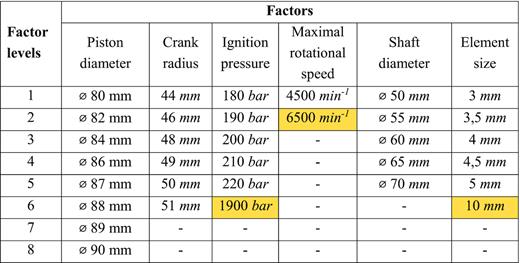
In the following subchapters, the parameters, which served to create the dataset, are presented in detail through tables and pictures. The orange highlighted cells in the tables contain the implausible values.
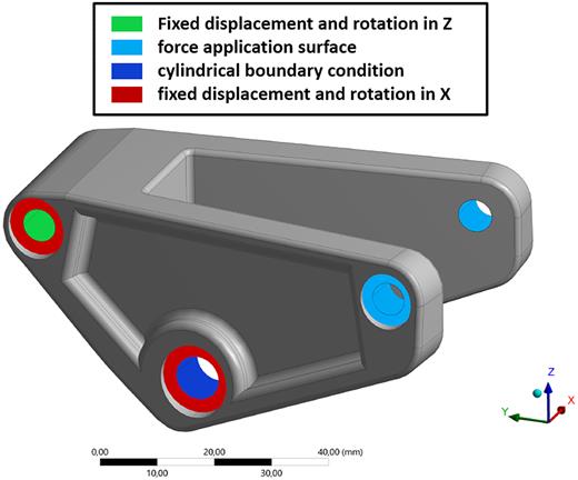
A1.1 Inline-skate rail
Setup of the FE simulation for the inline-skate rail.
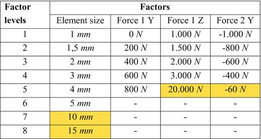
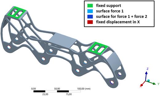
A1.2 Mountain bike bracket
Setup of the FE simulation for the mountain bike bracket.
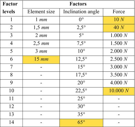
A1.3 Crankshaft
To convert the values from Table A3 into a simulation model, some calculations are necessary first. On the one hand, the compensation force has to be calculated and, on the other hand, the gas force.
|$r$| crank radius
|${d_{rod}}$| connecting rod bearing diameter
|${b_{cheek}}$| cheek width
|$\beta $| opening angle of the balance weight
|${\rho _{steel}}$| steel density
|${r_C}$| radius of the center of mass (Formula A.3)
|$n$| rotational speed
The calculation of the forces caused by the gas forces of the six cylinders of the combustion engine can be calculated using the following sources (Wackerbauer, Stuppy, & Meerkamm, 2009; Koehler & Flierl, 2011; Basshuysen & Schaefer, 2014). It is a relation, which consists of the following input variables:
- Crank angle
- Number of cylinders
- Piston diameter
- Ignition pressure
- Connecting rod length
- Connecting rod ratio (here = 0; 3)
- Crank radius
- Piston mass
- Connecting rod mass
- The rotational speed of the crankshaft
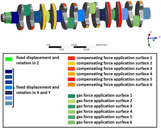
Setup of the FE simulation for the crankshaft.
