Inference from the small scales of cosmic shear with current and future Dark Energy Survey data

Abstract

Cosmic shear is sensitive to fluctuations in the cosmological matter density field, including on small physical scales, where matter clustering is affected by baryonic physics in galaxies and galaxy clusters, such as star formation, supernovae feedback, and active galactic nuclei feedback. While muddying any cosmological information that is contained in small-scale cosmic shear measurements, this does mean that cosmic shear has the potential to constrain baryonic physics and galaxy formation. We perform an analysis of the Dark Energy Survey (DES) Science Verification (SV) cosmic shear measurements, now extended to smaller scales, and using the Mead et al. (2015) halo model to account for baryonic feedback. While the SV data has limited statistical power, we demonstrate using a simulated likelihood analysis that the final DES data will have the statistical power to differentiate among baryonic feedback scenarios. We also explore some of the difficulties in interpreting the small scales in cosmic shear measurements, presenting estimates of the size of several other systematic effects that make inference from small scales difficult, including uncertainty in the modelling of intrinsic alignment on non-linear scales, ‘lensing bias’, and shape measurement selection effects. For the latter two, we make use of novel image simulations. While future cosmic shear data sets have the statistical power to constrain baryonic feedback scenarios, there are several systematic effects that require improved treatments, in order to make robust conclusions about baryonic feedback.

gravitational lensing: weak, large-scale structure of Universe

1 INTRODUCTION

The high galaxy number densities of typical weak lensing data sets, and the subsequent large number of galaxy pairs with ∼arcminute angular separation, make shear two-point correlations a powerful probe of the density field on ≲1 Mpc physical scales, where density fluctuations are highly non-linear. The shear two-point signal depends on the matter power spectrum, P_δ(k, z), which describes statistically the two-point clustering of matter as a function of scale (the physical wavevector, k) and redshift, z. We need to be able to predict P_δ(k, z) accurately, given a set of cosmological parameters, if we are to infer anything about those cosmological parameters.

For k ≳ 0.1 h Mpc⁻¹, N-body simulations are required to predict the non-linear matter clustering. Epic computational demands come from the requirement that the simulations are large enough to include the effects of large-scale power and subdue sampling variance, and have sufficiently high resolution to reach the large k required to make predictions of e.g. the small-scale cosmic shear signal (see e.g. Heitmann et al. 2010 for discussion of the simulation requirements for matter power spectrum prediction). To make predictions for a range of different cosmological models, we require the simulations to be re-run many times i.e. a suite of simulations is required. The most advanced example of this sort of suite is the Extended Coyote Universe simulations (Heitmann et al. 2014), which was used to build a matter power spectrum emulator accurate to 5 per cent up to k = 10 h Mpc⁻¹ and z = 4. These types of simulations are often called ‘dark matter only’ simulations, although ‘gravity-only’ would perhaps be more appropriate since they do have Ω_b > 0, but do not include the effects of non-gravitational physics. As we discuss below, non-gravitational or ‘baryonic’ physics may have a significant effect on the matter clustering on non-linear scales.

White (2004), Zhan & Knox (2004), and Huterer & Takada (2005) first identified the potential of baryonic physics to contaminate the cosmic shear signal, using simple theoretical models to predict several percent changes in the shear power spectrum at multipoles l ≳ 1000. Jing et al. (2006), Rudd et al. (2008), Hearin & Zentner (2009), Guillet, Teyssier & Colombi (2010), Casarini et al. (2012) used hydrodynamic simulations to account for the many complex baryonic processes such as active galactic nuclei (AGNs) feedback, gas cooling, and supernovae feedback which affect the matter power spectrum. Hydrodynamic simulations incorporate gas physics by including fluid dynamics as well as gravity, and are consequently more computationally expensive than gravity-only simulations. To fully simulate the relevant baryonic physical processes would require far higher resolution than can currently be achieved for the large volumes required for cosmology, so they are added using ‘sub-grid’ prescriptions. Since we have incomplete understanding of these physical processes, these sub-grid prescriptions need to be calibrated against observables. For example in the state-of-the-art EAGLE simulations (Schaye et al. 2015; Crain et al. 2015), stellar and AGNs feedback efficiency is calibrated to reproduce the observed z ∼ 0 galaxy stellar mass function (GSMF). While this guarantees that the feedback implementation is accurate in its effect on the z ∼ 0 GSMF, it does not guarantee the feedback implementation is accurate in its effect on e.g. the z ∼ 1 GSMF or the non-linear matter power spectrum. One might conclude that although hydrodynamic simulations can give us indications of the size and scale dependence of baryonic effects on the matter power spectrum, they are not yet sufficiently advanced to make predictions at the level of accuracy required for precision cosmology.

Various works have made use of the overwhelmingly large simulations (OWLS, Schaye et al. 2010), a suite of hydrodynamic simulations incorporating a variety of baryonic physics scenarios, for assessing the possible impact of baryonic physics on cosmic shear. van Daalen et al. (2011) measure matter power spectra from the different OWLS simulations which Semboloni et al. (2011) propagate to the shear two-point functions, finding deviations from the dark matter only case as large as 10–20 per cent for shear correlation functions ξ₊(θ = 1 arcmin) and ξ₋(θ = 10 arcmin).

Most previous cosmic shear studies have either ignored baryonic effects or discarded small scales from their analysis to reduce any potential bias from baryonic effects (see e.g. Kitching et al. 2014; MacCrann et al. 2015 for the latter approach). Recently however, Joudaki et al. (2016) performed a tomographic analysis of the CFHTLenS (Heymans et al. 2012) data, and marginalized over the possible baryonic feedback on the matter power spectrum, using a one free parameter version of the Mead et al. (2015) halo model (see Section 3 for further details). Unlike this work, their aim is to investigate the much discussed (e.g. Planck Collaboration XVI 2013; Battye & Moss 2014; MacCrann et al. 2015) tension with the Planck cosmic microwave background (CMB) constraints, rather than attempting to differentiate baryonic feedback scenarios, and they do not report constraints on baryonic feedback models.

Kitching et al. (2016) also investigate the tension between CFHTLenS and Planck by fixing the cosmological parameters to best-fitting values from Planck Collaboration XIII (2016b), and constraining various weak lensing nuisance parameters using the CFHTLenS data, including those sensitive to baryonic effects and intrinsic alignments. When allowing a free intrinsic alignment amplitude, they demonstrate a weak preference for a decrement in the matter power spectrum at small scales (compared to the no-baryonic feedback prediction), but no significant evidence for baryonic feedback. Harnois-Déraps et al. (2015) also use the CFHTLenS data to investigate baryonic feedback by fixing the cosmological parameters to best-fitting WMAP9 (Hinshaw et al. 2013) values, and constraining a 15 free parameter fitting formula describing deviations in the matter power spectrum due to baryonic feedback.

Most recently, Hildebrandt et al. (2016) use the same prescription as Joudaki et al. (2016) to marginalize over uncertainty due to baryonic feedback in their cosmic shear analysis of KiDS¹ survey data. Viola et al. (2015) also use KiDS weak lensing data, but use the tangential shear signal around galaxy groups. They compare the group mass as a function of BCG luminosity to predictions from the OWLS simulations, and observe a decrement in group mass at high luminosity that favours the prediction of the OWLS simulation containing AGNs feedback.

The Dark Energy Survey Collaboration et al. (2016) (DES16 henceforth) presented cosmological constraints from 150 deg² of Dark Energy Survey Science Verification (DES-SV) data. Using DECam (Flaugher et al. 2015), the final DES survey will image an area around 30 times this size. The DES-SV galaxy shear catalogues are described in Jarvis et al. (2016), the photometric redshift estimates in Bonnett et al. (2016), and the shear two-point measurements in Becker et al. (2016). They used the matter power spectra from van Daalen et al. (2011) to calculate a set of minimum angular scales on which to use the measured shear correlation functions, that would reduce any bias due to baryons to below the level of the statistical errors. This paper is motivated by the significant signal to noise (S/N) that this procedure wastes. Fig. 1 demonstrates this; it shows the total S/N of the DES-SV non-tomographic shear correlation functions ξ_±(θ), as a function of θ_min(ξ_±), the minimum scales used in ξ_±(θ). The red star marks the minimum scales used in DES16, and it is clear that more S/N (from ∼8 up to ∼13) can be gained by reducing these minimum scales. Even if astrophysical uncertainties are such that we cannot reliably infer cosmological parameters from the small-scale cosmic shear signal, it may be possible to learn about the astrophysical effects themselves. Therefore, it is tempting to try and exploit the extra S/N by including the small scales, and attempting to model the effects of baryons.

Figure 1.

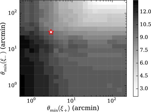
S/N of the DES-SV non-tomographic correlation functions ξ_±(θ), as a function of the minimum scale use in ξ_±, θ_min(ξ_±). The red outlined star marks the minimum scales used in DES16; clearly there is further signal to be exploited by reducing the minimum scales used.

In Section 2, we present new DES-SV cosmic shear measurements, using the galaxy shape catalogues described in Jarvis et al. (2016). These measurements are extended to smaller scales than those used in Becker et al. (2016) and DES16. In Section 3, we review some methods for modelling or parametrizing the effect of baryons on the matter power spectrum, including the extended halo model of Mead et al. (2015), and apply the Mead et al. (2015) model to these new cosmic shear measurements. We also forecast the potential of the final DES 5-yr (Y5) data to constrain this model.

Although baryonic effects may be the largest, there are several additional systematic effects that arise on small scales, which we describe in Section 4. We estimate several of these, and test their impact on the DES Y5 forecasted results. First, the observed (two-point) cosmic shear signal is usually considered to be sensitive only to second-order correlations in the underlying density field (and hence can be written as an integral over the matter power spectrum, see e.g. Bartelmann & Schneider 2001). In Section 4.1, we describe the corrections at third order in the density field that become significant on small scales. Meanwhile, the removal of blended objects during shape measurement can introduce a selection bias on the cosmic shear signal at small scales (Hartlap et al. 2011); we call this ‘blend-exclusion bias’, and investigate this effect using image simulations in Section 4.2. A further possible complication in interpreting the small-scale signal is intrinsic alignments, for which the successful large-scale models such as the (non-linear–) linear alignment (LA) model (Catelan, Kamionkowski & Blandford 2001; Hirata & Seljak 2004; Bridle & King 2007) are likely to break down; we discuss this in Section 4.3. Finally, we note that constraints from cosmic shear will of course be cosmology dependent, and one would expect the constraints on baryonic physics to be most degenerate with other phenomena that produce a scale-dependent change in the matter power spectrum, for example massive neutrinos. We investigate this degeneracy in Section 4.4.

2 SMALL-SCALE EXTENDED DES-SV SHEAR CORRELATION FUNCTIONS

In this section, we extend the DES-SV shear correlation function measurements to smaller scales. Fig. 2 shows measurements of the shear correlation functions ξ_± in 15 angular bins between 0.5 and 300 arcmin, in the same three redshift bins described in Becker et al. (2016) and DES16 (0.30 < z_mean < 0.55, 0.30 < z_mean < 0.55, and 0.55 < z_mean < 1.30, where z_mean is the mean of the photometric redshift PDF). We follow DES16 by excluding angular scales greater than 60 arcmin from ξ₊, to reduce the impact of additive systematics. There is a significant signal at scales down to 0.5 arcmin, particularly for the highest redshift bin. At scales less than a few arcminutes shape-noise, which arises from the uncorrelated intrinsic (unsheared) shapes of galaxies, is the dominant contribution to the covariance, so the data points are only weakly correlated. We conservatively choose 0.5 arcmin as the smallest separation used. While there still may be some signal below this, shape measurement systematics due to blending may become important.

Figure 2.

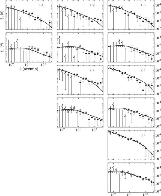
Shear correlation functions, ξ_±(θ) from DES-SV data, now using a data vector extended to smaller scales than in DES16 (open symbols indicate these smaller scales). The redshift bin pairing is shown in the upper right corner of each ξ₊ panel, and the corresponding ξ₋ measurement in the panel below. The solid line in each panel is the prediction using the Planck 2015 cosmology described in Section 3.2, and using the Takahashi et al. (2012) version of halofit (Smith et al. 2003). The dashed line shows the prediction from the OWLS AGN matter power spectrum (see Section 2 for details.)

The original DES16 cosmic shear analysis used a covariance matrix calculated from 126 mock survey simulations, as described in Becker et al. (2016). Becker et al. (2016) discussed the limitations on the accuracy of the parameter constraints that can be achieved when the number of simulation realizations is not much greater than the number of data points in the data vector (Dodelson & Schneider 2013; Taylor, Joachimi & Kitching 2013). For the extended tomographic data vector that we use in this work, this requirement is clearly not satisfied. We therefore use a covariance inferred from lognormal realizations of the lensing convergence across the survey area.

On large scales, the weak lensing convergence field (and therefore shear fields) is well described by Gaussian statistics, so a simple approximation to the cosmic shear covariance can be obtained by generating many Gaussian random shear fields with the expected shear power spectrum, and computing a sample covariance matrix using the same method as on the mocks. Since generation of the Gaussian realizations is very fast, the covariance uncertainty due to having a finite number of realizations can be made negligible. On smaller scales, the convergence field is sensitive to non-linearities in the density field, and the Gaussian approximation is no longer a good approximation. However, Taruya et al. (2002) and Takahashi et al. (2011) demonstrate that lognormal statistics provide a good description of the convergence field, while Hilbert, Hartlap & Schneider (2011) demonstrate that a covariance matrix obtained under the lognormal approximation results in very accurate confidence intervals on cosmological parameters, even when using sub-arcminute scales. Clerkin et al. (2016) found that the probability distribution function of both galaxy overdensity and convergence in the DES-SV data could be well approximated as lognormal, although they only investigated large (>10 arcmin) scales.

It is probable that the non-Gaussian terms in the covariance will be more accurately accounted for using the halo model (Peacock & Smith 2000; Seljak 2000), as in e.g. Sato et al. (2009), Takada & Hu (2013), and Eifler et al. (2014), which is a more physically motivated analytic description for the non-Gaussianities. However, accounting for the survey mask is likely to be more difficult in this approach.

3 MODELLING BARYONIC EFFECTS ON THE MATTER POWER SPECTRUM

3.1 Modelling approaches

We know from hydrodynamic simulations that baryonic physics can have a significant effect on the matter power spectrum at small scales. However, as described in Section 1, given the uncertainty in what physical processes to add to the simulations at the sub-grid level (as well as the uncertainties due to different implementations of the same sub-grid physics), the magnitude, scale dependence, and redshift dependence of the effect is very uncertain. In order to extract any information from the small scales, a model or nuisance parametrization that is sufficiently flexible to describe the baryonic effects, is required. Judging how flexible is ‘sufficiently’ flexible is always a challenge when assessing the suitability of a nuisance parametrization. The fact that a nuisance parametrization is required means that we lack knowledge about the physical process. However, deciding on a parametrization and priors on the nuisance parameters requires assumptions (presumably based on some knowledge) about the same physical process.

In the case of baryonic effects on the matter power spectrum, hydrodynamic simulations arguably provide a level of knowledge sufficient to provide the basis of a nuisance parametrization, or usefully test the flexibility of a modelling approach. The proposal of Eifler et al. (2015) makes this assumption; they propose using principal component analysis (PCA) to identify modes with the most variance between multiple simulations with different baryonic treatments. These modes can then be projected out of the analysis, providing a way of retaining only the information unaffected by baryonic effects that is more sophisticated than e.g. simply imposing a minimum angular scale.

More recently, Foreman, Becker & Wechsler (2016) present a method for using cosmic shear to constrain the matter power spectrum in a fairly model independent way; by allowing deviations from the dark matter only P_δ(k, z) at grid points in k and z. They demonstrate that using PCA to identify the best-constrained modes allows a decrease in the number of free parameters used, while retaining most of the information on any power spectrum deviation.

Another approach is to use a theoretical model for the matter power spectrum, with some physically motivated free parameters to account for possible baryonic effects. Zentner, Rudd & Hu (2008) and Hearin & Zentner (2009) showed that the effect of baryons on the matter power spectrum could be qualitatively reproduced in the halo model framework. The halo model (Peacock & Smith 2000; Seljak 2000) is an analytic model for the matter distribution in the Universe, that, given its simplicity, is extremely successful at reproducing the matter power spectrum, even on non-linear scales. The model assumes that all matter is contained in spherical haloes. The halo radial density profile is assumed to depend only on the mass of the halo. The statistical properties of the matter field are then set by three inputs: (i) the relation between the halo density profile and mass, (ii) the number density of haloes of a given mass, and (iii) the large-scale distribution of haloes, which just depends on the linear matter power spectrum. The halo density profile is usually taken to be the NFW profile (Navarro, Frenk & White 1996), which for a given mass, has one free parameter, the concentration. Input (i) is then the ‘concentration–mass relation’. Input (ii) is the halo mass function, the fraction of haloes in a given mass range. Both the concentration–mass relation and the halo mass function can be calibrated using N-body simulations.

Mead et al. (2015) use the halo model as a basis for which to tackle the problem of predicting the non-linear matter power spectrum. They first implement various adjustments to the basic halo model described above which are required to accurately predict the dark matter only matter power spectrum. With these adjustments, they achieve a 5 per cent matter power spectrum accuracy for k ≤ 10 h Mpc⁻¹, z ≤ 2, which they judge by comparison with the Coyote Universe simulations. In fact, the accuracy exceeds 2 per cent apart from around scales of k = 0.2 h Mpc⁻¹ where damping of the BAO is important, which they do not attempt to model.

They further extend this halo model to account for baryonic effects. We will refer to this extended halo model as the ‘M+15’ model. Since baryonic physics are likely to change the internal structure of haloes, but have a lesser effect on their positions or total masses, they propose two extra nuisance parameters to allow for the former. First, they allow to vary A, the amplitude in the concentration–mass relation i.e. increasing A makes haloes of all masses more concentrated. The second free parameter is η₀, which they call the ‘halo bloating parameter’, since it produces a (mass-dependent) bloating of the halo profile. To describe the effect of η₀, we first define

\begin{equation} \nu \equiv \frac{\delta _{\rm c}}{\sigma (R(M))}, \end{equation}

(1)

where δ_c is the linear theory overdensity collapse threshold and σ(R(M)) is the linear theory density variance in spheres of radius R that on average contain mass M. So ν < 1 haloes can be categorized as low mass, while ν > 1 haloes can be categorized as high mass. The halo profile in Fourier space, W(k, M) is modified as

\begin{equation} W(k,M) \rightarrow W(\nu ^\eta k, M), \end{equation}

(2)

where η = η₀ − 0.3σ₈(z). The result is that low-mass (ν < 1) haloes are more concentrated when η > 0 and more bloated when η < 0, while conversely high-mass (ν > 1) haloes are more bloated when η > 0 and more concentrated when η < 0. Fig. 3 shows the fractional change in the density profile of low- and high-mass haloes for positive and negative η. The figure demonstrates that the change in a ν = 0.6 (i.e. low-mass) halo profile due to setting η = 0.1 is the same as the change in a ν = 1.67 (i.e. high-mass) halo profile due to setting η = −0.1.

Figure 3.

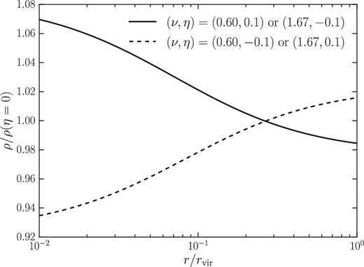
The fractional change in the halo density profile (as a function of radius in units of the virial radius of the η = 0 halo) due to non-zero η = η₀ − 0.3σ₈(z), for a high-mass (ν > 1) and low-mass halo (ν < 1). η₀ is one of the two free parameters in the Mead et al. (2015) halo model (see Section 3 for more details).

They test this parametrization by fitting the model to matter power spectra from three of the OWLS simulations, and in all cases achieve similar accuracy (∼<2 per cent up to k = 10 h Mpc⁻¹, apart from the BAO wiggles) in the matter power spectrum as for the dark matter only case (at the cost of these two extra nuisance parameters). The three OWLS simulations used are the ‘REF’, ‘DBLIM’, and ‘AGN’ simulations. The ‘REF’ simulation contains radiative cooling and heating, stellar evolution, chemical enrichment, stellar winds, and supernova feedback. The ‘AGN’ simulation is similar to the ‘REF’ simulation but additionally contains feedback from AGN. The ‘DBLIM’ simulation is again similar to ‘REF’ but has additional supernovae energy in wind velocity, and a top heavy initial mass function at high pressure. See Schaye et al. (2010) for detailed description of these simulations. We note here that the recent study of Cui et al. (2016) indicates that the methodology used in the OWLS simulations suite should be thought of as one of several that have not yet demonstrated convergence. That study shows that the even the sign of the effect on halo internal mass structure varies among simulation methods. Our use of OWLS as a reference in this work should be considered as illustrative of the potential magnitude of these complex effects.

To implement the M+15 model, we use HMCode,² code made publicly available by Mead et al. (2015), and included in the CosmoSIS (Zuntz et al. 2015) package. We use the CosmoSIS framework for all parameter inference in this work.

3.2 Constraints from DES-SV

Fig. 4 shows the constraints on A and η₀ from the DES-SV cosmic shear measurements described in Section 2. As well as the two halo model parameters, the same set of systematics parameters as used in DES16 are marginalized over: a redshift bin shift parameter per redshift bin, δz_i; a multiplicative shear bias per redshift bin, m_i; and an intrinsic alignment amplitude, A_IA. For the purple contour labelled ‘fiducial’, the intrinsic alignment model used is the ‘non-linear–linear alignment’ (NLA) model of Bridle & King (2007), which was the fiducial model used in DES16. As in DES16, Gaussian priors of width 0.05 are used for the δz_i and m_i, and a uniform prior [−5,5] on A_IA is used. Cosmological parameters are fixed to the Planck Collaboration XIII (2016b) ‘Planck TT + lowP’ values. The allowed ranges of the parameters A and η₀ are those plotted, which Mead et al. (2015) showed to be comfortably wide enough to span the space of simulations considered there.

Figure 4.

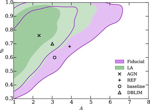
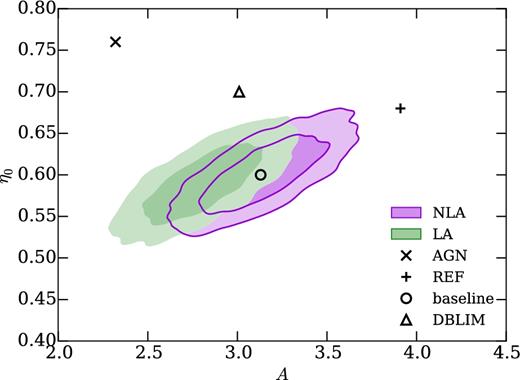
DES-SV cosmic shear 1σ and 2σ constraints on the two nuisance parameters of the M+15 halo model (Mead et al. 2015). The data vector has been extended to smaller scales than the original analysis (DES16). The purple filled and outlined contour is the fiducial analysis, the same three redshift bins as DES16, and angular scales in the range 0.5–300 arcmin. The green filled contour models galaxy intrinsic alignments using the LA model (Catelan et al. 2001; Hirata & Seljak 2004) rather than the NLA model (Bridle & King 2007) used for the fiducial analysis. The black markers show the best-fitting parameters for several different OWLS simulations, calculated by Mead et al. (2015). The plus is ‘REF’, the cross is ‘AGN’, the triangle is ‘DBLIM’, and the circle is for no baryonic effects (see Schaye et al. 2010; Mead et al. 2015 for descriptions of the OWLS simulation names).

Although the constraints from DES-SV are fairly weak, the high A, low η₀ region of the parameter space is strongly disfavoured. Shown as black marks are the best-fitting halo model parameters to various cosmological simulations, as estimated by Mead et al. (2015): the circle is the (A, η₀) which they find to be the best fit to the Coyote Universe simulations, which do not contain baryonic feedback effects; we call this the ‘baseline’ case. The plus is the best fit (A, η₀) for the OWLS ‘REF’ simulation, which contains radiative cooling and heating, stellar evolution, chemical enrichment, stellar winds, and supernova feedback (see Schaye et al. 2010 for detailed descriptions of the OWLS simulations). The cross is the best fit (A, η₀) for the OWLS ‘AGN’ simulation, which is similar to the ‘REF’ simulation, but additionally contains feedback from AGN. The triangle is the best fit (A, η₀) for the OWLS ‘DBLIM’ simulation, which is again similar to ‘REF’, but has additional supernovae energy in wind velocity, and a top heavy initial mass function at high pressure.

Note that we do not constrain the likelihood of the OWLS simulations directly – rather the parameters of the M+15 halo model, which we assume is flexible enough to account for a wide range of baryonic effects. So when we say e.g. ‘the AGN model is disfavoured with X per cent confidence’, we really mean the (A, η₀) preferred by the OWLS AGN simulation is disfavoured with X per cent confidence. Given the success of the M+15 model in encapsulating the different OWLS simulations, we believe this is a reasonable way to report constraints, but it is important to be clear that our constraints are on the halo model parameters, rather than on the OWLS simulations directly.

For the AGN model, the preferred (A, η₀) lies on the contour of equal-probability containing 22.8 per cent of the posterior probability. We define the quantity C_M, for baryonic model M with |$(A,\eta _0)=(A^{\rm M},\eta _0^{\rm M})$|⁠, as the percentage of the posterior weight contained within the contour of equal posterior on which |$(A^{\rm M},\eta _0^{\rm M})$| lies. So C_AGN = 22.8 per cent. A model M with C_M of 95 per cent would be considered disfavoured with 95 per cent confidence. We find C_baseline = 82.9 per cent, C_DBLIM = 52.0 per cent and C_REF = 86.9 per cent, so none of the models are strongly disfavoured by the DES-SV cosmic shear data.

4 PREDICTED BARYONIC CONSTRAINTS FROM DES COSMIC SHEAR AND SMALL-SCALE SYSTEMATICS

While current cosmic shear data such as DES-SV only weakly constrains models of baryonic physics and its effects on the Universe's matter distribution, upcoming data sets will have far greater statistical power. The final DES data set, which we call ‘Y5’, since it will be composed of 5 yr of data, will be around 30 times larger in area than DES-SV. The purple filled/outlined contour in Fig. 5 shows the expected constraints on the M+15 halo model parameters from Y5 cosmic shear data. To perform this forecast we use as a ‘simulated’ data vector a theoretical prediction, and then run an MCMC parameter estimation analysis, as would be performed on a measured data vector. The simulated data vector has no baryonic physics added. The covariance and data vector are the same as that used in Foreman et al. 2016, which assumes a five tomographic bin analysis, over the angular range 0.5 < θ < 300 arcmin, with eight galaxies per square arcminute, and an area of 5000 deg². The covariance matrix was computed using CosmoLike (Eifler et al. 2014; Krause & Eifler 2016). Again (and unless otherwise specified), we fix cosmological parameters to the Planck Collaboration XIII (2016b) values described in Section 3.2 (we explore variations in cosmological parameters, including the neutrino mass, in Section 4.4).

Figure 5.

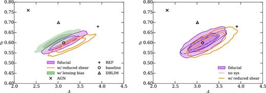
Expected constraints (assuming the baseline model) on the M+15 model parameters from DES Year 5 cosmic shear. We assume a tomographic data vector with five redshift bins, using an angular range 0.5 < θ < 300 arcmin. Left-hand panel: the weak lensing nuisance parameters described in Section 3.2 are not marginalized over. The purple (outlined and filled) contours show the constraints with no systematics added to the simulated data vector, hence the input halo model parameters are correctly recovered. For the orange outlined (green filled) contours, we include a correction to the simulated data vector for reduced shear (lensing bias). When fitting the simulated data vector, we do not include either correction, hence the contours are shifted, and the inferred halo model parameters are somewhat biased. Right-hand panel: the purple and orange contours are the same as in the left-hand panel, except now marginalizing over the 11 weak lensing nuisance parameters (a δz_i and m_i per redshift bin and an intrinsic alignment amplitude A_IA), hence the constraints on the halo model parameters become weaker, and the bias due to ignoring the reduced shear correction becomes less significant. For comparison, the black dotted line shows the constraints without marginalizing over the weak lensing (WL) nuisance parameters (i.e. the purple contour in the left-hand panel). In both panels, the black markers are the same as in Fig. 4.

In the left-hand panel, no weak lensing systematics nuisance parameters (i.e. the δz_i, m_i, and A_IA described in Section 3.2) are marginalized over. In the right-hand panel these systematics parameters are included, although we now use Gaussian priors of width 0.02 for the δz_i and m_i, which we hope will be justified by higher quality data and improved data reduction tools. Even without such improvements, it is likely that future DES analyses will combine shear two-point measurements with galaxy–galaxy lensing and galaxy clustering measurements which will tighten constraints on systematic parameters (see e.g. Joachimi & Bridle 2010; Zhang, Pen & Bernstein 2010). In order to make robust conclusions about baryonic physics, we must ensure that any other uncertainties or systematic biases in the small-scale cosmic shear signal are accounted for. The green filled contour in Fig. 4 shows an example of this. For these contours an alternative model of galaxy intrinsic alignments is assumed, the linear alignment model (Catelan et al. 2001; Hirata & Seljak 2004, see Section 4.3 for more details). When this intrinsic alignment model is assumed, the REF and baseline M+15 halo model parameters (the ‘+’ in Fig. 4) are now disfavoured, with C_baseline = 97.0 per cent and C_REF = 97.2 per cent. This is a simple demonstration that even with DES-SV data, including uncertainties in the intrinsic alignment modelling is important.

In this section, we discuss various theoretical/systematic uncertainties that can potentially bias conclusions from small-scale cosmic shear measurements, including intrinsic alignments (Section 4.3). We use the Y5 forecast to quantify the importance of the various systematic effects. In particular, we calculate the credible interval, C_truth in the A − η₀ plane, on which the true (A, η₀) (i.e. those used to generate the simulated data vector) lie, when we include a particular systematic in the simulated data vector, but do not include it in the modelling. A C_truth value of 90 per cent would indicate that ignoring that systematic would result in the true values of (A, η₀) being ruled out with 90 per cent confidence. So C_truth quantifies the severity of the bias caused by a particular systematic effect.

4.1 Reduced shear and lensing bias

In this section, we consider two contributions to the observed cosmic shear signal that arise from third-order correlations of the convergence or equivalently third order in the gravitational potential, Ψ (usually only the second-order correlations are considered, in which case the cosmic shear signal can be written as a projection of the matter power spectrum, see e.g. Bartelmann & Schneider 2001). Krause & Hirata (2010) investigate corrections up to O(Ψ⁴), and although the O(Ψ⁴) terms will be non-negligible for future surveys, the O(Ψ³) terms are around an order of magnitude larger, and so we only consider the latter here. The observable in cosmic shear is the two-point correlation of the observed ellipticity, |$\langle \epsilon ^{\rm {obs}}(\boldsymbol {x})\epsilon ^{\rm {obs}}(\boldsymbol {x^{\prime }})\rangle$|⁠. It is usually assumed that this is an unbiased estimate of the two-point correlation of the shear |$\langle \gamma (\boldsymbol {x})\gamma (\boldsymbol {x})\rangle$|⁠. Ignoring intrinsic alignments, we describe below two O(Ψ³) reasons why this is not quite correct.

First, the ellipticity that we measure is actually an estimate of the reduced shear, g, which is related to the shear via

\begin{equation} g(\boldsymbol {x})=\frac{\gamma (\boldsymbol {x})}{1-\kappa (\boldsymbol {x})} \approx \gamma (\boldsymbol {x})(1+\kappa (\boldsymbol {x})). \end{equation}

(3)

This requires a ‘reduced shear’ correction to the predicted signal, which is derived in the Appendix, following Shapiro (2009).

Secondly, we only observe the shear at the position of galaxies, so when we compute a ‘shear’ two-point correlation function, we are effectively computing the correlation function of the galaxy density-weighted reduced shear, g^obs, given by

\begin{equation} g_{{\rm obs}}(\boldsymbol {x}) = (1+\delta _{{\rm obs}}(\boldsymbol {x}))g(\boldsymbol {x}), \end{equation}

(4)

where |$\delta _{{\rm obs}}(\boldsymbol {x})$| is the observed galaxy overdensity at |$\boldsymbol {x}$|⁠. We consider two ways in which an observed galaxy overdensity at angular coordinate |$\boldsymbol {\theta }$| and radial coordinate χ can arise (apart from random fluctuations). First there could be an overdensity in the galaxy number at |$(\boldsymbol {\theta },\chi )$| e.g. if there is a cluster there. Secondly, there could be a change in the number density of galaxies that we can observe, due to lensing magnification e.g. if there is a cluster at |$(\boldsymbol {\theta },\chi ^{\prime }<\chi )$|⁠. The first leads to the ‘source-lens clustering’ (Bernardeau 1998; Hamana et al. 2002), which is zero in the Limber limit (see the Appendix). The second effect produces what is known as lensing bias (or sometimes ‘magnification bias’), and we derive an expression for it in the Appendix, following Schmidt et al. (2009).

4.1.1 The reduced shear correction

From Shapiro (2009), the reduced shear correction to the projected shear power spectrum for tomographic bin pairs i and j is given by

\begin{equation} \delta _{\rm {red}} C_{ij}^{\kappa }(l)=\ 2\int \frac{\mathrm{d}^2{l^{\prime }}\,}{(2\pi )^2} {\rm cos}(2\phi _{l^{\prime }}-2\phi _{l}) \ B_{ij}(\boldsymbol {l^{\prime }},\boldsymbol {l}-\boldsymbol {l^{\prime }},\boldsymbol {-l}), \end{equation}

(5)

where

\begin{eqnarray} B_{ij}(\boldsymbol {l_1},\boldsymbol {l_2},\boldsymbol {l_3}) &=& \frac{1}{2}\int \frac{\mathrm{d}{\chi }\,}{\chi ^4}W_i(\chi )W_j(\chi )[W_i(\chi )+W_j(\chi )] \nonumber\\ &&\times \, B_{\delta }(\boldsymbol {k_1}, \boldsymbol {k_2}, \boldsymbol {k_3}; \chi ), \end{eqnarray}

(6)

|$B_{\delta }(\boldsymbol {k_1}, \boldsymbol {k_2}, \boldsymbol {k_3}; \chi )$| is the matter bispectrum, and W_i(χ) is the radial lensing kernel for redshift bin i. We use the fitting formula for the matter bispectrum from Scoccimarro & Couchman (2001). Fig. 6 shows the effect of reduced shear on the shear power spectrum, for the same redshift bins as used in the DES-SV analysis in Section 3.2. The fractional bias is ∼1 per cent at l of a few hundred and ∼10 per cent at l of 10⁴.

Figure 6.

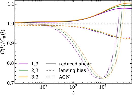
The fractional difference in the shear power spectrum due to reduced shear (solid lines) and lensing bias (dashed lines) are compared to that from the OWLS AGN model (dotted lines). We used the DES-SV tomographic redshift distributions, and for clarity only show the correlations with the highest redshift bin.

Fig. 7 shows the effect of the reduced shear on the shear correlation functions ξ_±, which at 1 arcmin is ∼2 per cent for ξ₊ and ∼8 per cent for ξ₋. Hence, the reduced shear correction, although not as large as the effect of baryons in the OWLS AGN model, is non-negligible for small-scale cosmic shear measurements.

Figure 7.

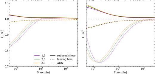
The fractional difference in the projected shear correlation functions ξ_± due to reduced shear (solid lines) and lensing bias (dashed lines) are compared to that from the OWLS AGN model (dotted lines). We used the DES-SV tomographic redshift distributions, and for clarity only show the correlations with the highest redshift bin.

4.1.2 The lensing bias

In the Appendix, we derive (drawing heavily on Schmidt et al. 2009) the lensing bias correction to the shear power spectrum, which for a pair of redshift bins i and j is

\begin{equation} \delta _{{\rm lensing}}C_{ij}^{\kappa }(l) = \int \frac{\mathrm{d}^2{l^{\prime }}\,}{(2\pi )^2} \cos (2\phi _{l^{\prime }}-2\phi _l) B^q_{ij}(\boldsymbol {l^{\prime }},\boldsymbol {l}-\boldsymbol {l^{\prime }},-\boldsymbol {l}), \end{equation}

(7)

where

\begin{eqnarray} B^q_{ij}(\boldsymbol {l_1},\boldsymbol {l_2},\boldsymbol {l_3})&=& \frac{1}{2}\int \frac{\mathrm{d}{\chi }\,}{\chi ^4}W_i(\chi )W_j(\chi )[q_iW_i(\chi )+q_jW_j(\chi )] \nonumber\\ &&\times B_{\delta }(\boldsymbol {l_1}/\chi , \boldsymbol {l_2}/\chi , \boldsymbol {l_3}/\chi ; \chi ). \end{eqnarray}

(8)

The quantity q_i is given by

\begin{equation} q_i=2\beta _f+\beta _r-2, \end{equation}

(9)

where

\begin{eqnarray} \beta _f \equiv \int \mathrm{d}{r}\, \int \mathrm{d}{f}\, \frac{\mathrm{\partial} \epsilon (f,r)}{\mathrm{\partial} (\ln (f))}\Phi (f,r), \end{eqnarray}

(10)

\begin{eqnarray} \beta _r \equiv \int \mathrm{d}{r}\, \int \mathrm{d}{f}\, \frac{\mathrm{\partial} \epsilon (f,r)}{\mathrm{\partial} (\ln (r))}\Phi (f,r). \end{eqnarray}

(11)

ε(f, r) is the survey selection function in galaxy flux, f, and size, r; Φ(f, r) is the true galaxy distribution in flux and size. We make use of the Balrog simulations (Suchyta et al. 2016) to estimate ε(f, r) and Φ(f, r). Balrog is a method for simulating observed galaxy catalogues, by injecting simulated objects with known properties into real survey images. The resulting ‘simulated’ images therefore contain many of the important properties of the real data, including observational systematics that would be otherwise difficult to simulate, as well as a small³ number of extra injected objects. The properties (both morphology and multiband fluxes) of the inserted objects are based on COSMOS observations, which also have accurate redshifts. By running the same catalogue creation software (in this case SExtractor, Bertin & Arnouts 1996) on these simulated images as is run on the real data, and then repeating the injection and catalogue creation process many times over, we can estimate the mapping from the true properties of a galaxy to the properties estimated by SExtractor in our galaxy catalogues. For example, we can estimate the probability of detecting a galaxy with a particular true flux and size, or more generally, the survey selection function as defined above, ε(f, r). We estimate Φ(f, r) and ε(f, r) as follows.

• We start with the SV ngmix (Sheldon 2014) shape catalogue (that was used in DES16), and the Balrog catalogue used in Suchyta et al. (2016), the latter of which contains both ‘observed’ fluxes and sizes i.e. those estimated by SExtractor, as well as true fluxes and sizes (those used when drawing the simulated objects into the DES images) and redshifts. Note that the observed sizes are point spread function (PSF)-convolved.

• For a given redshift bin of the SV ngmix data, we re-weight the Balrog data to have the same redshift distribution. Then we compute Φ(f, r) using weighted kernel-density-estimation (KDE) in the true flux and size of these weighted Balrog objects.

• We then re-weight the Balrog data to have the same observed flux and size distribution as the ngmix shape catalogue, for that particular redshift bin. For the observed flux and size we use the i-band SExtractor quantities MAG_AUTO and FLUX_RADIUS to do this and make use of the hep_ml package⁴ to perform Gradient Boosting⁵ re-weighting. With this new set of weights, we again use weighted KDE to estimate Φ^obs(f, r), given by

  \begin{equation} \Phi ^{\rm {obs}}(f,r)=\epsilon (f,r)\Phi (f,r). \end{equation}

  (12)

• We then estimate ε(f, r) as Φ^obs(f, r)/Φ(f, r).

4.1.3 Impact on signal and baryonic constraints

Having estimated Φ(f, r) and ε(f, r), the expressions in equa-tions (10) and (11) can be calculated and substituted into (9). We find q₁ = −1.02 ± 0.02, q₂ = −0.79 ± 0.01, q₃ = −0.64 ± 0.01 (the errors are derived by jackknifing the galaxies used for the KDEs). We use these q values to estimate the lensing bias contribution to the shear power spectra (Fig. 6, dashed lines), and the shear correlation functions (Fig. 7, dashed lines), for the redshift binning used in the DES-SV analysis. The lensing bias correction has the same scale dependence and similar magnitude to the reduced shear correction, but the negative values of q_i make it negative, partially cancelling out the reduced shear correction.

We now turn to the DES Y5 forecast to demonstrate the importance of accounting for the reduced shear and lensing bias. We perform simulated likelihood analyses where either the reduced shear correction or lensing bias correction is used to generate the ‘simulated’ data vector from theory, but not included in the modelling during parameter estimation. For the lensing bias, we assume q_i = −1 for all redshift bins for simplicity (but the procedure outline in Section 4.1.2 could be used with the DES Y5 data in order to estimate the q_i). Fig. 5 shows the shift in the contours in the (A, η₀) plane, due to ignoring either the reduced shear or lensing bias. In the left-hand panel, the case where no lensing systematics (i.e. the nuisance parameters used in the analysis of Section 3.2 accounting for multiplicative shear bias, photometric redshift bias, or intrinsic alignments) are marginalized over, the shifts in the halo model parameters from ignoring these effects are significant. For the reduced shear case (green filled contour), we find C_truth = 97.4 per cent, implying that the true values of (A, η₀) would be excluded with 97.4 per cent confidence if the reduced shear correction were ignored. As expected, the shift due to ignoring lensing bias is almost identical, but in the opposite direction. However, the shifts in the contours are still small compared to the differences between the different OWLS simulations in the (A, η₀) plane, so we concluded that marginalizing over any uncertainty (due to e.g. imperfect knowledge of the bispectrum, or the survey selection function) in the reduced shear or lensing bias corrections will not significantly reduce the power of DES Y5 to differentiate between the OWLS models used here.

For the right-hand panel of Fig. 5, the weak lensing nuisance parameters are now marginalized over, increasing the size of the contours, and reducing the significance of the M+15 parameter shifts. In this case, when ignoring the reduced shear, we find C_truth = 43.6 per cent, so the recovered parameters are within ‘1σ’ of the truth.

In these calculations, we have assessed the impact of reduced shear and lensing bias separately; however, in real weak lensing data they will of course both be present. While the magnitude of the reduced shear correction depends only on the redshift distribution of the sources and the cosmological model, the magnitude of the lensing bias correction depends on the complex way in which galaxies are selected for shear estimation, which will vary between different weak lensing data sets. We have estimated the q_i for the DES-SV data to be ∼− 1, leading to a correction that largely cancels the reduced shear correction, and for the DES Y5 forecast we took q_i = −1, which would lead to exact cancellation with the reduced shear correction (i.e. a C_truth = 0 per cent when lensing bias and reduced shear are considered simultaneously). However, equation (9) indicates that the q_i need not be close to −1 and can be positive or negative, so one cannot assume that the reduced shear and lensing bias will largely cancel in the general case.

4.2 Blend-exclusion bias: estimates using BCC-UFig

Estimating the shear of a noisy, PSF-convolved galaxy is a notoriously difficult problem (see e.g. Mandelbaum et al. 2014). The difficulty is further increased if the galaxy has a closely neighbouring object, since the shear estimation is likely to be disrupted by the contaminating light from the neighbour. We can categorize objects as blended if they overlap at a particular isophotal level, for example SExtractor identifies objects by first finding groups of contiguous pixels above some detection threshold, and then deciding how many objects to split these pixels into (this decision is part of the deblending process). If that number of objects is more than one, then these objects will be flagged as blended objects. Shape or photometry estimates (required for photo-z estimation) from these objects should be used with caution. Indeed in the DES-SV shape catalogues (Jarvis et al. 2016), we excluded any objects that SExtractor judged to be blended.

Hartlap et al. (2011) realized that this exclusion of blended objects produces a selection bias by the following mechanism: blended objects are more likely to be in crowded regions of the sky (e.g. along the same line of sight as a cluster), and these crowded regions will have higher convergence than average (e.g. because of the aforementioned cluster). Therefore by excluding blended objects, we are undersampling the higher convergence regions of the sky, compared to the less-crowded, lower convergence regions. Thus, we will underestimate the shear two-point signal, especially on small scales, where sensitivity to those crowded, high convergence regions is highest. We call this effect blend-exclusion bias. Hartlap et al. (2011) estimated the magnitude of this effect by starting with a mock weak lensing catalogue (produced from ray-traced N-body simulations), and cutting out galaxies based on various criteria; for example, they apply what they call the ‘FIX’ criterion, where if a pair of galaxies is separated by less than some angle θ_FIX, they exclude one of those galaxies. For θ_FIX = 2 arcsec(5 arcsec), they find a −1(−2) per cent bias in ξ₊(θ = 1 arcmin), and a −2(−7) per cent bias in ξ₋(θ = 1 arcmin).

These sorts of criteria give a useful indication of the expected bias; however, on real data, the criteria we use for deciding whether to use a galaxy are often not so well defined. As explained above, in the DES-SV analyses (e.g. Becker et al. 2016, DES16; Jarvis et al. 2016) SExtractor was used to decide whether a galaxy is blended, and the behaviour of SExtractor is dependent on the details of the images, for example the PSF, the noise levels, and the distribution of galaxy fluxes and sizes. These details are not captured in the approach taken by Hartlap et al. (2011), since they do not simulate survey images. The approach we take uses the blind cosmology challenge-ultrafast image generator (BCC-UFig) image simulations (Chang et al. 2015), which allows investigation of the behaviour of the same selections we use on the real data. The BCC-UFig image simulations start with a cosmological mock galaxy simulation (the BCC, Busha et al. 2013), with lensing information from ray-tracing (Becker 2013). This is used as input to an image generator (the UFig, Bergé et al. 2013; Bruderer et al. 2016) that produces images with properties like noise levels and PSF well matched to DES data (see Chang et al. 2015; Leistedt et al. 2016). The BCC-UFig catalogues are then produced by running SExtractor on these simulated images, with a configuration designed to match that run on the DES-SV data by the DES data management pipeline.

We estimate the size of the blend-exclusion bias as follows.

• We start with the DES-SV shape catalogue split into the three redshift bins presented in Becker et al. (2016) and re-weight the BCC-UFig catalogue to have the same observed magnitude, size, and redshift distribution. We use the i-band SExtractor quantities MAG_AUTO and FLUX_RADIUS to match the magnitude and size distributions since we have these for both the SV data, and the BCC-UFig catalogues. We call this re-weighted catalogue the ‘full’ UFig catalogue.

• We measure the shear correlation functions ξ_±(θ) from the full UFig catalogue, using the true input shears to the simulation. We use the true input shears, since the aim here is to isolate the selection bias, rather than study any other shape measurement biases. We call this signal |$\xi _{\pm }^{{\rm full}}(\theta )$|⁠.

• We then impose a cut on the SExtractor flag value in the full UFig catalogue that removes blended objects or those with bright, close neighbours (around 15 per cent of the objects). This is the same cut that was applied to the DES-SV shape catalogues for weak lensing analyses. We re-weight the resulting catalogue to have the same redshift distribution as the full UFig catalogue, and call this the ‘cleaned’ UFig catalogue. We measure the shear correlation functions from the cleaned UFig catalogue, and call this signal |$\xi _{\pm }^{{\rm cleaned}}(\theta )$|⁠. Then the fractional bias is |$\xi _{\pm }^{{\rm cleaned}}(\theta )/\xi _{\pm }^{{\rm full}}(\theta )-1$|⁠.

The ratio |$\xi _{\pm }^{{\rm cleaned}}(\theta )/\xi _{\pm }^{{\rm full}}(\theta )$| is plotted in Fig. 8. We show only correlations with the highest redshift bin for clarity, but there is no clear redshift dependence of the bias. For ξ₊, the bias reaches ∼3 per cent at 1 arcmin, while for ξ₋, the bias reaches this level at 10–20 arcmin. Thus, the effect is of the same order as found in Hartlap et al. (2011) and is similar in magnitude and scale dependence to the reduced shear and lensing bias effects. Thus, we conclude that the blend-exclusion bias will produce a similar level of bias in the inferred M+15 halo model parameters as the reduced shear and lensing bias.

Figure 8.

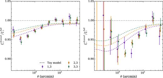
A measurement of blend-exclusion bias using BCC-UFig. The ratio of the shear correlation functions estimated from the BCC-UFig simulations after removing SExtractor blends, to the correlation functions using the full galaxy sample. The two samples were weighted to have the same redshift distributions, and the true input shears to the simulations were used to calculate ξ_±, in order to isolate the selection effect. For clarity only correlations with the highest redshift bin (bin 3) are shown. The dashed lines show the prediction of the toy model described in Section 4.2

This similarity is perhaps not surprising, since this blend-exclusion bias can be thought of as a form of source-lens clustering whereby the exclusion of blended objects produces changes in the source galaxy density that are correlated with the density field; this is also the result of the lensing bias described in Section 4.1.2. Motivated by this similarity, we formulate a toy model for the blend-exclusion bias. In this toy model, we assume the probability of a galaxy at |$\boldsymbol {\theta }$| being blended depends only on the amount of light from neighbours in that area of sky. This can be quantified as the excess flux density (above the mean flux density), which we will call |$\kappa _{{\rm flux}}(\boldsymbol {\theta })$|⁠. Consider the contribution to |$\kappa _{{\rm flux}}(\boldsymbol {\theta })$| from a comoving volume element dV  at comoving distance χ. The contribution to the excess flux in area element dΩ  is

\begin{equation} \Delta \kappa _{{\rm flux}}(\boldsymbol {\theta },\chi ) \mathrm{d}{\chi }\, \mathrm{d}{\Omega }\, = \frac{\delta _{{\rm L}}(\boldsymbol {\theta },\chi )}{4\pi d_{\rm L}(\chi )^2} \mathrm{d}{V,}\, \end{equation}

(13)

where d_L(χ) is the luminosity distance. δ_L(θ, χ) is the comoving volume luminosity overdensity at (θ, χ), given by

\begin{equation} \delta _{{\rm L}}(\boldsymbol {\theta },\chi ) = \frac{L(\boldsymbol {\theta },\chi )-\bar{L}(\chi )}{\bar{L}(\chi )}, \end{equation}

(14)

where |$L(\boldsymbol {\theta },\chi )$| is the luminosity density at |$(\boldsymbol {\theta },\chi )$| and |$\bar{L}(\chi )$| is the mean luminosity density at comoving distance χ. The comoving volume element can be replaced using dV = χ²dχ dΩ, yielding

\begin{equation} \Delta \kappa _{{\rm flux}}(\boldsymbol {\theta },\chi ) \mathrm{d}{\chi }\, = \frac{\delta _{{\rm L}}(\boldsymbol {\theta },\chi )}{4\pi d_{\rm L}(\chi )^2} \chi ^2 \mathrm{d}{\chi }\,. \end{equation}

(15)

We make the assumption that the luminosity overdensity δ_L(θ, χ) is proportional to the matter overdensity δ(θ, χ). This would be the case if galaxies did not evolve with redshift, and had luminosity-independent bias (hence we call this a toy model!). Then

\begin{equation} \Delta \kappa _{{\rm flux}}(\boldsymbol {\theta },\chi ) \mathrm{d}{\chi }\, \propto \frac{\chi ^2\delta (\boldsymbol {\theta },\chi )}{d_{\rm L}(\chi )^2} \mathrm{d}{\chi }\, \end{equation}

(16)

and

\begin{equation} \kappa _{{\rm flux}}(\boldsymbol {\theta }) \propto \int \mathrm{d}{\chi }\, \frac{\chi ^2\delta (\boldsymbol {\theta },\chi )}{d_{\rm L}(\chi )^2}. \end{equation}

(17)

We assume that the observed galaxy overdensity (i.e. the fractional excess in galaxy number density) due to blending is proportional to the excess flux density |$\kappa _{{\rm flux}}(\boldsymbol {\theta })$|⁠, so using equation (17),

\begin{equation} \delta _{{\rm obs}}^{{\rm blend}}(\boldsymbol {\theta }) = \alpha \kappa _{{\rm flux}}(\boldsymbol {\theta }) = \alpha \int \mathrm{d}{\chi }\, \frac{\chi ^2\delta (\boldsymbol {\theta },\chi )}{d_{\rm L}(\chi )^2} \end{equation}

(18)

where α is a constant of proportionality, which we expect to be negative, since an excess in flux density should lead to more blending, and so a negative |$\delta _{{\rm obs}}^{{\rm blend}}$|⁠.

Like the convergence, |$\delta _{{\rm obs}}^{{\rm blend}}(\boldsymbol {\theta })$| is a projection in χ of the matter overdensity, δ, but with a kernel

\begin{equation} W^{\prime }(\chi ) = \frac{\alpha \chi ^2}{d_{\rm L}^2(\chi )} = \frac{\alpha \chi ^2}{(1+z(\chi ))^2 D_A^2(\chi )} \end{equation}

(19)

instead of the lensing kernel. So the effect on the shear power spectrum can be calculated in exactly the same way as the reduced shear correction, but replacing the lensing kernels [W_i(χ) + W_j(χ)] in equations (5) and (6), with 2W΄(χ). The dashed lines in Fig. 8 show the prediction of this toy model, with α = −0.1 showing qualitative agreement with the measurement from BCC-UFig.

It worth noting finally that the magnitude of this selection bias (and indeed the lensing bias described in Section 4.1.2) will depend on the estimator used for the two-point cosmic shear signal. For example a pixel-based estimator (i.e. where the mean shear is calculated in pixels on the sky, and then these mean values are used in the two-point statistic) may be less susceptible to biases that arise from variations in the source density. However, if the pixels are weighted by the number of galaxies in each pixel, to approximate inverse-variance weighting, then in the small pixel limit, the pixel estimator will be equivalent to the estimators used here.

4.3 Intrinsic alignments

The observed intrinsic alignments of bright red galaxies (see e.g. Singh, Mandelbaum & More 2015) on linear and mildly non-linear scales are well described by theoretical models that assume tidal alignment, in which the galaxy ellipticity is assumed to align with the local tidal field. The simplest of these is the LA model (Catelan et al. 2001; Hirata & Seljak 2004), in which the alignment is assumed to be linear in the linear tidal field, which leads to an alignment power spectrum that depends on the linear matter power spectrum. The LA model has only one free parameter, an amplitude A_IA that is of order unity (this is just called ‘A’ in DES16). A popular variation is the NLA model, which was introduced by Bridle & King (2007), who replaced the linear matter power spectrum with the non-linear matter power spectrum; this model has been more successful than the LA model in fitting observations on mildly non-linear scales (e.g. Joachimi & Schneider 2010), despite the fact that it does not include all non-linear corrections in a consistent way. Blazek, Vlah & Seljak (2015) systematically include non-linear corrections (at one-loop order in perturbation theory) to the LA model, producing a model that provides a further improved fit in the mildly non-linear regime. Meanwhile, it is commonly assumed that the intrinsic alignments of spiral galaxies, which are primarily angular momentum supported, are better described by theories based on tidal torquing (White 1984); these are also known as quadratic alignment models (Crittenden et al. 2001; Mackey, White & Kamionkowski 2002; Hirata & Seljak 2004). Blazek et al. (in preparation) propose a perturbative model for populations of mixed galaxy type that consistently includes both tidal alignment and tidal torque-type contributions. Halo model-based intrinsic alignment models (see e.g. Schneider & Bridle 2010) are likely to be more successful in the fully non-linear 1-halo regime. A detailed study of intrinsic alignments on non-linear scales is beyond the scope of this work; we perform a simple test to gauge the order of the uncertainty in this section.

We use the difference between the LA model and the NLA model as a proxy for the uncertainty in the behaviour of intrinsic alignments on non-linear scales. The green contours in Fig. 4 shows the DES-SV constraints on the halo model parameters when the LA model is assumed rather than the fiducial NLA model (purple filled/outlined contours). The is a ∼1σ shift in the contours, towards the low A favoured by the ‘AGN’ model. This can be understood as follows: the wide redshift binning means that the dominant effect of intrinsic alignments is the negative ‘GI’ term. The NLA model therefore produces a larger negative contribution at small scales than the LA term. When the LA model is assumed, a lower A (leading to reduced halo concentration, and thus a reduced small-scale cosmic shear signal), is required to fit the observed signal.

A similar shift in contours is observed for the Y5 forecast, shown as the green contours in Fig. 9. In this case, the ‘simulated’ data vector uses the NLA model, with A_IA = 0.5, with the green contours resulting from fitting this data vector using the LA model. In this case, C_truth = 82.8 per cent so the shift is significant. One could imagine marginalizing over extra nuisance parameters to account for the uncertainty in the intrinsic alignment modelling on non-linear scales. As a simple example, we implement an intrinsic alignment model that is a mixture of the LA and NLA models, with the amount of non-linearity determined by a free parameter α_nl, such that the intrinsic ellipticity power spectrum, P_II(k, z) becomes

\begin{equation} P_{\rm {II}}(k,z) = \alpha _{\rm {nl}} P_{\rm {II}}^{\rm {NLA}}(k,z) + (1 - \alpha _{\rm {nl}}) P_{\rm {II}}^{\rm {LA}}, \end{equation}

(20)

and similarly for the intrinsic ellipticity-density cross spectrum P_GI. Despite this extra flexibility, the degradation of the M+15 parameter constraints is negligible. While this particular model may not be very realistic, this result suggests that the future cosmic shear data will have the power to constrain additional nuisance parameters which account for the uncertainty of intrinsic alignments on non-linear scales, without significantly degrading the constraints on the M+15 model parameters, and therefore models of baryonic physics.

Figure 9.

Expected constraints from DES Y5 on M+15 halo model parameters given different assumptions about intrinsic alignments. The purple (filled and lined) contour is the same as in the right-hand panel of Fig. 5. For the green filled contour, the LA model is used to fit the simulated data vector, instead of the NLA model which was used to generate the simulated data vector (with A_IA = 0.5). This results in biased recovery of the M+15 halo model parameters.

4.4 Degeneracy with cosmology

Thus far, we have fixed all cosmological parameters, however, there will be some degeneracy between the halo model parameters and the cosmological parameters. In particular, neutrino mass also produces scale-dependent change in the matter power spectrum, so we expect it to have some degeneracy with baryonic feedback. Natarajan et al. (2014) investigate this degeneracy, concluding that one can infer biased values of the neutrino mass from cosmic shear if baryonic feedback is not accounted for. We now repeat the Y5 forecast, but allowing cosmological parameters (Ω_m, Ω_b, H₀, n_s, A_s) to vary, while combining with Planck CMB constraints [specifically we use the low-l TEB and high-l TT likelihoods presented in Planck Collaboration XI (2016a)]. Note that we do not include CMB lensing information. There is only a small increase in the errorbars on the halo model parameters A and η₀ (7 per cent increase in |$\sqrt{\sigma _{A}\sigma _{\eta _0}}$|⁠). When the neutrino density Ω_νh² is additionally marginalized over, there is a further 23 per cent increase in |$\sqrt{\sigma _{A}\sigma _{\eta _0}}$|⁠. This degradation is due to the presence of degeneracy between the neutrino mass and the halo model parameters, as demonstrated in Fig. 10. Hence, we conclude that marginalizing over cosmological parameters, including the neutrino mass, will not greatly reduce the ability of DES Y5 data to constrain baryonic effects on the matter power spectrum, when combining with Planck CMB data.

Figure 10.

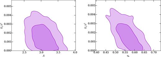
Forecasted degeneracy between the neutrino energy density Ω_νh² and the M+15 halo model parameters, for DES Year 5 combined with Planck CMB constraints. For the simulated data vector, we assumed Ω_νh² = 6 × 10⁻⁴, approximately the minimal value allowed by solar neutrino oscillation observations (Fukuda et al. 1998), and the halo model parameters corresponding to the baseline case (A = 3.13, η₀ = 0.60).

5 DISCUSSION

The small scales of cosmic shear measurements are rich in both signal-to-noise and difficult-to-model systematic uncertainties. Baryonic effects present the largest systematic uncertainty, with 10–20 per cent deviations from the dark matter only case on arcminute scales predicted by some hydrodynamic simulations. The prospects for gaining useful cosmological information from the small scales of cosmic shear do not look bright given these uncertainties. However, small-scale cosmic shear measurements do still provide unique observational constraints on the small-scale matter clustering, since cosmic shear is the observational probe that can most directly probe the total matter distribution on small scales. These can be straightforwardly compared to e.g. the predictions from hydrodynamic simulations, or analytic models.

We note that cosmic shear is not the only way to exploit weak lensing data sets, which (either alone or in combination with galaxy redshift surveys) can also be used for galaxy clustering measurements or probing the cross-correlation between galaxy number density and shear. Viola et al. (2015) have already shown the sensitivity of the latter to baryonic feedback. Furthermore, the addition of galaxy clustering and number density–shear cross-correlation information will constrain some of the systematic effects that reduce the effectiveness of cosmic shear-alone analyses, such as intrinsic alignments (Joachimi & Bridle 2010) and photometric redshift uncertainties (Zhang et al. 2010; Samuroff et al. 2017).

While current cosmic shear data has limited constraining power (such as the DES-SV constraints presented in Section 3.2), we have shown that information from DES Y5 data has the potential to distinguish possible baryonic scenarios, producing information that could be fed back into future hydrodynamic simulations, which in turn will hopefully improve our ability to model the small-scale clustering. In order to make robust conclusions about baryonic physics from small-scale cosmic shear however, other non-negligible systematics should be accounted for, such as the reduced shear correction, lensing bias, blend-exclusion bias, and uncertainties due to intrinsic alignment modelling. We have demonstrated that all of these effects, if not accounted for, can significantly bias the inferred small-scale matter power spectrum. In particular, we have shown that these effects will bias the parameters of the Mead et al. (2015) halo model; however, this conclusion will be true for whatever model or prescription is used to account for the uncertainties in the small-scale matter power spectrum.

While the theoretical framework for modelling the reduced shear is well established, a prediction for the matter bispectrum is required, which on non-linear scales may also depend on the baryonic feedback. We have demonstrated how novel image simulations can be used to estimate the effect of lensing bias (which also requires a prediction of the matter bispectrum), and the blend-exclusion bias. Intrinsic alignment modelling on non-linear scales is still extremely uncertain; however, we have shown the potential of future cosmic shear data to constrain uncertainty in the non-linear intrinsic alignment modelling at the same time as the baryonic effects. Finally, although the baryonic effects on the matter power spectrum are to some extent degenerate with the effect of massive neutrinos, we have shown that marginalizing over neutrino mass does not greatly reduce the potential constraining power of DES Y5 cosmic shear data, when it is combined with Planck CMB data.

Acknowledgments

We thank to Simon Foreman and Neil Jackson for useful discussion. We also thank to Alex Mead for help with HMcode and Elisabeth Krause for producing the halo model covariance from Cosmolike.

We are grateful for the extraordinary contributions of our CTIO colleagues and the DECam Construction, Commissioning and Science Verification teams in achieving the excellent instrument and telescope conditions that have made this work possible. The success of this project also relies critically on the expertise and dedication of the DES Data Management group.

Funding for the DES Projects has been provided by the U.S. Department of Energy, the U.S. National Science Foundation, the Ministry of Science and Education of Spain, the Science and Technology Facilities Council of the United Kingdom, the Higher Education Funding Council for England, the National Center for Supercomputing Applications at the University of Illinois at Urbana-Champaign, the Kavli Institute of Cosmological Physics at the University of Chicago, the Center for Cosmology and Astro-Particle Physics at the Ohio State University, the Mitchell Institute for Fundamental Physics and Astronomy at Texas A&M University, Financiadora de Estudos e Projetos, Fundação Carlos Chagas Filho de Amparo à Pesquisa do Estado do Rio de Janeiro, Conselho Nacional de Desenvolvimento Científico e Tecnológico and the Ministério da Ciência, Tecnologia e Inovação, the Deutsche Forschungsgemeinschaft, and the Collaborating Institutions in the DES. The DES data management system is supported by the National Science Foundation under Grant Number AST-1138766.

The Collaborating Institutions are Argonne National Laboratory, the University of California at Santa Cruz, the University of Cambridge, Centro de Investigaciones Enérgeticas, Medioambientales y Tecnológicas-Madrid, the University of Chicago, University College London, the DES-Brazil Consortium, the University of Edinburgh, the Eidgenössische Technische Hochschule (ETH) Zürich, Fermi National Accelerator Laboratory, the University of Illinois at Urbana-Champaign, the Institut de Ciències de l'Espai (IEEC/CSIC), the Institut de Física d'Altes Energies, Lawrence Berkeley National Laboratory, the Ludwig-Maximilians Universität München and the associated Excellence Cluster Universe, the University of Michigan, the National Optical Astronomy Observatory, the University of Nottingham, The Ohio State University, the University of Pennsylvania, the University of Portsmouth, SLAC National Accelerator Laboratory, Stanford University, the University of Sussex, and Texas A&M University.

The DES participants from Spanish institutions are partially supported by MINECO under grants AYA2012-39559, ESP2013-48274, FPA2013-47986, and Centro de Excelencia Severo Ochoa SEV-2012-0234 and SEV-2012-0249. Research leading to these results has received funding from the European Research Council under the European Union Seventh Framework Programme (FP7/2007-2013) including ERC grant agreements 240672, 291329, and 306478.

This paper has gone through internal review by the DES collaboration.

1

http://kids.strw.leidenuniv.nl

2

https://github.com/alexander-mead/HMcode

3

Sufficiently small that we need not consider any interaction between the injected objects.

4

https://github.com/arogozhnikov/hep_ml

5

https://en.wikipedia.org/wiki/Gradient_boosting

APPENDIX: THIRD-ORDER CORRECTIONS TO SHEAR–SHEAR CORRELATIONS

In cosmic shear, we attempt to measure the two-point correlation of the shear, possibly between two different redshift bins i and j

\begin{equation} \xi _{i,j} = \langle \gamma _i(\boldsymbol {x})\gamma _j(\boldsymbol {x^{\prime }}) \rangle . \end{equation}

(A1)

Contributions to shear two-point correlation at third order in the density field arise from two effects

• We observe the reduced shear,

  \begin{equation} g(\boldsymbol {x})=\frac{\gamma (\boldsymbol {x})}{1-\kappa (\boldsymbol {x})}\approx (1+\kappa (\boldsymbol {x}))\gamma (\boldsymbol {x}). \end{equation}

  (A2)
• We can only estimate the shear at positions of galaxies. So any statistic (e.g. the mean shear or ξ_±) estimated from the measured shears will effectively be using the galaxy number density-weighted reduced shear:

  \begin{eqnarray} g^{{\rm obs}}(\boldsymbol {x}) &= (1 + \delta _{{\rm obs}}(\boldsymbol {x}))g(\boldsymbol {x})), \end{eqnarray}

  (A3)

  \begin{eqnarray} \quad\,\,\,&= (1 + \delta _{{\rm obs}}(\boldsymbol {x}))(1+\kappa (\boldsymbol {x}))\gamma (\boldsymbol {x}), \end{eqnarray}

  (A4)

  where |$\delta _{{\rm obs}}(\boldsymbol {x})$| is the observed overdensity in galaxy number at position |$\boldsymbol {x}$|⁠. This observed overdensity can be due to a true change in the number density of galaxies at |$\boldsymbol {x}$| (for example due to the presence of a cluster), or due to a change in the observable number density due to lensing magnification (for example due to the presence of a cluster at lower redshift). The first effect leads to source-lens clustering (Bernardeau 1998; Hamana et al. 2002) and the second leads to lensing bias (Schmidt et al. 2009).

We start with the expression from Schmidt et al. (2009) for the expectation of the standard ξ_± estimator.

\begin{equation} \langle \xi _{ij}^{\mathrm{obs}}\rangle = \left\langle \frac{ g_i^{\mathrm{obs}}(\boldsymbol {x})g_j^{\mathrm{obs}}(\boldsymbol {x^{\prime }})}{1 + 2\overline{\delta _{{\rm obs}}} + \widehat{\delta _{{\rm obs}}\delta _{{\rm obs}}}}\right\rangle , \end{equation}

(A5)

where |$\overline{\delta _{{\rm obs}}}$| is the mean observed galaxy overdensity across the survey (negligible for a wide survey), |$\widehat{\delta _{{\rm obs}}\delta _{{\rm obs}}}$| is a mean product of overdensities smoothed over the bin width (ξ_gg(θ) in the limit of an infinite survey and narrow bin). Substituting for |$g_i^{\mathrm{obs}}$| from equa-tion (A4), the terms up to third order in γ, κ, or δ are

\begin{eqnarray} \langle \xi _{ij}^{\mathrm{obs}}\rangle &= &\langle \gamma _i(\boldsymbol {x})\gamma _j(\boldsymbol {x^{\prime }})\rangle \nonumber \\ &&+ \langle \kappa (\boldsymbol {x})\gamma _i(\boldsymbol {x})\gamma _j(\boldsymbol {x^{\prime }})\rangle + \langle \gamma _i(\boldsymbol {x})\kappa (\boldsymbol {x^{\prime }})\gamma _j(\boldsymbol {x^{\prime }})\rangle \nonumber \\ &&+ \langle \delta _{{\rm obs}}(\boldsymbol {x})\gamma _i(\boldsymbol {x})\gamma _j(\boldsymbol {x^{\prime }})\rangle + \langle \gamma _i(\boldsymbol {x})\delta _{{\rm obs}}(\boldsymbol {x^{\prime }})\gamma _j(\boldsymbol {x^{\prime }})\rangle . \end{eqnarray}

(A6)

The first line is the ‘true’ shear–shear signal. The second line is the reduced shear contribution, which is only zero if the convergence κ is not correlated with the shear at a given point on the sky, which is unlikely, since they are sourced by the same structure. The third line is the source-lens clustering (including ‘lensing bias’, since magnification contributes to δ_obs). This would be zero if there was no correlation between the source galaxy overdensity and the shear at a given point on the sky e.g. if source galaxies were randomly distributed.

For convenience, we label each term on the left-hand side of equation (A6) as follows

\begin{eqnarray} \langle \gamma ^{\mathrm{obs}}_i(\boldsymbol {l},\chi )\gamma ^{\mathrm{obs},*}_j(\boldsymbol {l^{\prime \prime }},\chi ^{\prime })\rangle &=& \langle \gamma _i(\boldsymbol {l},\chi )\gamma _j^{\ast }(\boldsymbol {l^{\prime \prime }},\chi ^{\prime })\rangle \nonumber\\ &&+ R_{ij} + R_{ji} + S_{ij} + S_{ji}, \end{eqnarray}

(A7)

where

\begin{eqnarray} R_{ij} &= \langle (\kappa _i\gamma _i)(\boldsymbol {l},\chi )\gamma _j^{\ast }(\boldsymbol {l^{\prime \prime }},\chi ^{\prime }))\rangle , \end{eqnarray}

(A8)

\begin{eqnarray} R_{ji} &= \langle \gamma _i(\boldsymbol {l},\chi )(\kappa _j\gamma _j)^{\ast }(\boldsymbol {l^{\prime \prime }},\chi ^{\prime })\rangle , \end{eqnarray}

(A9)

\begin{eqnarray} S_{ij} &= \langle (\delta _{{\rm obs},i}\gamma _i)(\boldsymbol {l},\chi )\gamma _j^{\ast }(\boldsymbol {l^{\prime \prime }},\chi ^{\prime }))\rangle , \end{eqnarray}

(A10)

\begin{eqnarray} S_{ji} &= \langle \gamma _i(\boldsymbol {l},\chi )(\delta _{{\rm obs},j}\gamma _j)^{\ast }(\boldsymbol {l^{\prime \prime }},\chi ^{\prime })\rangle , \end{eqnarray}

(A11)

and subscripts i and j denote shears/overdensities/convergences taken from redshift bins i and j. It is more convenient to compute these terms in Fourier space where the multiplicative adjustments to the shear become convolutions i.e.

\begin{eqnarray} (\kappa \gamma )(\boldsymbol {l}) &=& \int \frac{\mathrm{d}^2{l^{\prime }}\,}{(2\pi )^2} \gamma (\boldsymbol {l^{\prime }})\kappa (\boldsymbol {l}-\boldsymbol {l^{\prime }}), \end{eqnarray}

(A12)

\begin{eqnarray} (\delta _{{\rm obs}}\gamma )(\boldsymbol {l}) &=& \int \frac{\mathrm{d}^2{l^{\prime }}\,}{(2\pi )^2} \gamma (\boldsymbol {l^{\prime }}) \delta _{{\rm obs}}(\boldsymbol {l}-\boldsymbol {l^{\prime }}). \end{eqnarray}

(A13)

So

\begin{eqnarray} R_{ij} &=&\int \frac{\mathrm{d}^2{l^{\prime }}\,}{(2\pi )^2} \langle \gamma _i(\boldsymbol {l^{\prime }},\chi )\kappa _i(\boldsymbol {l}-\boldsymbol {l^{\prime }},\chi ) \gamma ^{\ast }_j(\boldsymbol {l^{\prime \prime }},\chi ^{\prime })\rangle , \end{eqnarray}

(A14)

\begin{eqnarray} R_{ji} &=&\int \frac{\mathrm{d}^2{l^{\prime }}\,}{(2\pi )^2} \langle \gamma _i(\boldsymbol {l},\chi )\gamma _j^{\ast }(\boldsymbol {l^{\prime }},\chi ^{\prime })\kappa _j(\boldsymbol {l^{\prime \prime }}-\boldsymbol {l^{\prime }},\chi ^{\prime })\rangle , \end{eqnarray}

(A15)

\begin{eqnarray} S_{ij} &= &\int \frac{\mathrm{d}^2{l^{\prime }}\,}{(2\pi )^2} \langle \delta _{{\rm obs},i}(\boldsymbol {l^{\prime }},\chi )\gamma _i(\boldsymbol {l}-\boldsymbol {l^{\prime }},\chi ) \gamma ^{\ast }_j(\boldsymbol {l^{\prime \prime }},\chi ^{\prime })\rangle , \end{eqnarray}

(A16)

\begin{eqnarray} S_{ji} &=&\int \frac{\mathrm{d}^2{l^{\prime }}\,}{(2\pi )^2} \langle \gamma _i(\boldsymbol {l},\chi )\gamma _j^{\ast }(\boldsymbol {l^{\prime }},\chi ^{\prime })\delta _{{\rm obs},j}^{\ast }(\boldsymbol {l^{\prime \prime }}-\boldsymbol {l^{\prime }},\chi ^{\prime })\rangle . \end{eqnarray}

(A17)

We use the following:

\begin{eqnarray} \gamma _i(\boldsymbol {l}) &= \mathrm{e}^{2\mathrm{i}\phi _l}\kappa _i(\boldsymbol {l}), \end{eqnarray}

(A18)

\begin{eqnarray} \kappa _i^{\ast }(\boldsymbol {l}) &= \kappa _i(-\boldsymbol {l}), \end{eqnarray}

(A19)

\begin{eqnarray} \delta _{{\rm obs},i}^{\ast }(\boldsymbol {l}) &= \delta _{{\rm obs},i}(-\boldsymbol {l}), \end{eqnarray}

(A20)

where ϕ_l is the angle made by |$\boldsymbol {l}$| with the x-axis, to obtain

\begin{eqnarray} R_{ij} &=&\int \frac{\mathrm{d}^2{l^{\prime }}\,}{(2\pi )^2} \mathrm{e}^{2\mathrm{i}(\phi _{l^{\prime }}-\phi _{l^{\prime \prime }})} \langle \kappa _i(\boldsymbol {l^{\prime }},\chi )\kappa _i(\boldsymbol {l}-\boldsymbol {l^{\prime }},\chi ) \kappa _j(\boldsymbol {-l^{\prime \prime }},\chi ^{\prime })\rangle,\nonumber \\ \end{eqnarray}

(A21)

\begin{eqnarray} R_{ji} &=&\int \frac{\mathrm{d}^2{l^{\prime }}\,}{(2\pi )^2} \mathrm{e}^{2\mathrm{i}(\phi _{l}-\phi _{l^{\prime }})} \langle \kappa _i(\boldsymbol {l},\chi )\kappa _j(\boldsymbol {-l^{\prime }},\chi ^{\prime }) \kappa _j(\boldsymbol {l^{\prime }-l^{\prime \prime }},\chi ^{\prime })\rangle,\nonumber \\ \end{eqnarray}

(A22)

\begin{eqnarray} S_{ij} &=&\int \frac{\mathrm{d}^2{l^{\prime }}\,}{(2\pi )^2} \mathrm{e}^{2\mathrm{i}(\phi _{l^{\prime }}-\phi _{l^{\prime \prime }})} \langle \kappa _i(\boldsymbol {l^{\prime }},\chi )\delta _{{\rm obs},i}(\boldsymbol {l}-\boldsymbol {l^{\prime }},\chi ) \kappa _j(\boldsymbol {-l^{\prime \prime }},\chi ^{\prime })\rangle,\nonumber \\ \end{eqnarray}

(A23)

\begin{eqnarray} S_{ji} &=&\int \frac{\mathrm{d}^2{l^{\prime }}\,}{(2\pi )^2} \mathrm{e}^{2\mathrm{i}(\phi _{l}-\phi _{l^{\prime }})} \langle \kappa _i(\boldsymbol {l},\chi )\kappa _j(-\boldsymbol {l^{\prime }},\chi ^{\prime }) \delta _{{\rm obs},j}(\boldsymbol {l^{\prime }}-\boldsymbol {l^{\prime \prime }},\chi ^{\prime })\rangle.\nonumber \\ \end{eqnarray}

(A24)

We can write the reduced shear terms R_ij and R_ji in terms of the convergence bispectrum, |$B_{(\kappa _1,\kappa _2,\kappa _3)}(\boldsymbol {l_1},\boldsymbol {l_2},\boldsymbol {l_3})$| defined as

\begin{eqnarray} \langle \kappa _i(\boldsymbol {l_1})\kappa _j(\boldsymbol {l_2}) \kappa _k,(\boldsymbol {l_3})\rangle &=& \ (2\pi )^2\delta _{\rm D}(\boldsymbol {l_1}+\boldsymbol {l_2}+\boldsymbol {l_3})B_{(\kappa _1,\kappa _2,\kappa _3)}\nonumber\\ &&\times\, (\boldsymbol {l_1},\boldsymbol {l_2},\boldsymbol {l_3}). \end{eqnarray}

(A25)

This can be related to the matter bispectrum using the Limber approximation

\begin{eqnarray} B_{(\kappa _1,\kappa _2,\kappa _3)}(\boldsymbol {l_1},\boldsymbol {l_2},\boldsymbol {l_3}) = \int \frac{\mathrm{d}{\chi }\,}{\chi ^4} W_1(\chi )W_2(\chi )W_3(\chi ) B_{\delta }(\boldsymbol {k_1}, \boldsymbol {k_2}, \boldsymbol {k_3}; \chi ),\!\!\!\!\!\!\nonumber\\ \end{eqnarray}

(A26)

where W_i(χ) is the lensing kernel for redshift bin i and |$\boldsymbol {k_1}=\boldsymbol {l_1}/\chi$| etc. Note the |$\delta _{\rm D}(\boldsymbol {l_1}+\boldsymbol {l_2}+\boldsymbol {l_3})$| enforces a triangle configuration of the three vectors. So R_ij and R_ji become

\begin{eqnarray} R_{ij} &=&\int \frac{\mathrm{d}^2{l^{\prime }}\,}{(2\pi )^2} \mathrm{e}^{2\mathrm{i}(\phi _{l^{\prime }}-\phi _{l^{\prime \prime }})} (2\pi )^2 B_{(\kappa _i,\kappa _i,\kappa _j)}(\boldsymbol {l^{\prime }},\boldsymbol {l}-\boldsymbol {l^{\prime }},\boldsymbol {-l}), \end{eqnarray}

(A27)

\begin{eqnarray} R_{ji} &=&\int \frac{\mathrm{d}^2{l^{\prime }}\,}{(2\pi )^2} \mathrm{e}^{2\mathrm{i}(\phi _{l}-\phi _{l^{\prime }})} (2\pi )^2 B_{(\kappa _i,\kappa _j,\kappa _j)}(\boldsymbol {l},\boldsymbol {-l^{\prime }},\boldsymbol {l^{\prime }-l}). \end{eqnarray}

(A28)

We can write the left-hand side of A7 as

\begin{equation} \langle \gamma _i(\boldsymbol {l})\gamma _j^{\ast }(\boldsymbol {l^{\prime \prime }})\rangle = \ (2\pi )^2\delta ^{\rm D}(\boldsymbol {l}-\boldsymbol {l^{\prime \prime }})C_{ij}^{\kappa }(l), \end{equation}

(A29)

so the change in |$C_{ij}^{\kappa }(l)$| due to reduced shear is

\begin{eqnarray} \delta _{\mathrm{red}} C_{ij}^{\kappa }(l)&=&[R_{ij}+R_{ji}]/(2\pi )^2 \nonumber \\ &=&\int \frac{\mathrm{d}^2{l^{\prime }}\,}{(2\pi )^2} \mathrm{e}^{2\mathrm{i}(\phi _{l^{\prime }}-\phi _{l})} \ B_{(\kappa _i,\kappa _i,\kappa _j)}(\boldsymbol {l^{\prime }},\boldsymbol {l}-\boldsymbol {l^{\prime }},\boldsymbol {-l}) \nonumber \\ &&+\, \mathrm{e}^{2\mathrm{i}(\phi _{l}-\phi _{l^{\prime }})} B_{(\kappa _i,\kappa _j,\kappa _j)}(\boldsymbol {l},-\boldsymbol {l^{\prime }},\boldsymbol {l^{\prime }}-\boldsymbol {l}). \end{eqnarray}

(A30)

We can arrive at equation 13 of Shapiro (2009) by taking the real part, assuming some symmetry properties of the convergence bispectrum [|$B(\boldsymbol {l_1},\boldsymbol {l_2},\boldsymbol {l_3})=B(-\boldsymbol {l_1},-\boldsymbol {l_2},-\boldsymbol {l_3})$| and |$B(\boldsymbol {l_1},\boldsymbol {l_2},\boldsymbol {l_3})=B(\boldsymbol {l_3},\boldsymbol {l_1},\boldsymbol {l_2})$|] and defining the ‘2-redshift convergence bispectrum’

\begin{eqnarray} B_{ij}(\boldsymbol {l_1},\boldsymbol {l_2},\boldsymbol {l_3})&=& \frac{1}{2}\int \frac{\mathrm{d}{\chi }\,}{\chi ^4}W_i(\chi )W_j(\chi )[W_i(\chi )+W_j(\chi )]\nonumber \\ &&\times \, B_{\delta }(\boldsymbol {k_1}, \boldsymbol {k_2}, \boldsymbol {k_3}; \chi ), \end{eqnarray}

(A31)

which in our notation is equal to

\begin{equation} \frac{1}{2}[B_{(\kappa _i,\kappa _i,\kappa _j)}(\boldsymbol {l_1},\boldsymbol {l_2},\boldsymbol {l_3}) + B_{(\kappa _i,\kappa _j,\kappa _j)}(\boldsymbol {l_1},\boldsymbol {l_2},\boldsymbol {l_3})]. \end{equation}

(A32)

Substituting into equation (A30)

\begin{equation} \delta _{\mathrm{red}} C_{ij}^{\kappa }(l)=\ 2\int \frac{\mathrm{d}^2{l^{\prime }}\,}{(2\pi )^2} {\rm cos}(2\phi _{l^{\prime }}-2\phi _{l}) \ B_{ij}(\boldsymbol {l^{\prime }},\boldsymbol {l}-\boldsymbol {l^{\prime }},\boldsymbol {-l}). \end{equation}

(A33)

We now move on to the S_ij and S_ji terms. Various things can cause a galaxy overdensity δ_obs, but we are concerned with ones that are correlated with the density field. These arise from two sources. The first and most obvious one is if the source galaxies trace the density field e.g. with some linear bias b_g

\begin{equation} \delta _{{\rm obs},i}(\boldsymbol {l},\chi )=N_i(\chi )b_g(\chi )\delta (\boldsymbol {l},\chi ). \end{equation}

(A34)

Then we have

\begin{eqnarray} S_{ij} &=&\int \frac{\mathrm{d}^2{l^{\prime }}\,}{(2\pi )^2} {\rm e}^{2i(\phi _{l^{\prime }}-\phi _{l^{\prime \prime }})} \langle \kappa _i(\boldsymbol {l^{\prime }},\chi )b_g(\chi )N_i(\chi )\nonumber\\ &&\times \, \delta (\boldsymbol {l}-\boldsymbol {l^{\prime }},\chi ) \kappa _j(\boldsymbol {-l^{\prime \prime }},\chi ^{\prime })\rangle . \end{eqnarray}

(A35)

In the Limber approximation (in which we assume density fluctuations at different radial distances are uncorrelated), this term goes to zero, by the following argument: |$\kappa _i(\boldsymbol {l^{\prime }},\chi )$| only depends on the density field for radial distances less than χ, and so is uncorrelated with |$\delta (\boldsymbol {l}-\boldsymbol {l^{\prime }},\chi )$|⁠. |$\kappa _j(\boldsymbol {-l^{\prime \prime }},\chi ^{\prime })$| gets contributions from density fluctuations all along the line of sight. Those produced by fluctuations at χ΄! = χ will be uncorrelated with |$\delta (\boldsymbol {l}-\boldsymbol {l^{\prime }},\chi )$|⁠, so for χ΄! = χ, |$\delta (\boldsymbol {l}-\boldsymbol {l^{\prime }},\chi )$| is correlated with neither |$\kappa _i(\boldsymbol {l^{\prime }},\chi )$| or |$\kappa _j(\boldsymbol {l^{\prime }},\chi ^{\prime })$|⁠. The contribution to |$\kappa _j(\boldsymbol {-l^{\prime \prime }},\chi ^{\prime })$| produced by fluctuations at χ΄ = χ will be correlated with |$\delta (\boldsymbol {l}-\boldsymbol {l^{\prime }},\chi )$|⁠, but uncorrelated with |$\kappa _i(\boldsymbol {l^{\prime }},\chi )$|⁠. In both these cases, one of the variables in the three-point correlator is uncorrelated with the other two, and since all variables have zero mean, the three-point correlation is zero. Hence for δ_obs(χ) satisfying 〈δ_obs(χ)δ(χ΄)〉 = δ^D(χ − χ΄)〈δ_obs(χ)δ(χ΄)〉, S_ij = S_ji = 0. This is the source-lens clustering term which is zero in the Limber approximation (see Valageas 2014 for a treatment beyond the Limber approximation).

From Schmidt et al. (2009), the lensing bias produces an observed galaxy overdensity |$\delta _{{\rm obs},i}(\boldsymbol {\theta },\chi ) = q_i\kappa _i(\boldsymbol {\theta },\chi )$| (to first order in κ), where q is a constant that depends on the survey selection function. In this case, S_ij = q_iR_ij, and we get the same result as in the reduced shear case, but for the q_i prefactors

\begin{eqnarray} \delta _{{\rm lensing}}C_{ij}^{\kappa }(l) &=&[q_iR_{ij}+q_jR_{ji}]/(2\pi )^2 \nonumber \\ &=& \int \frac{\mathrm{d}^2{l^{\prime }}\,}{(2\pi )^2} \cos (2\phi _{l^{\prime }}-2\phi _l) B^q_{ij}(\boldsymbol {l^{\prime }},\boldsymbol {l}-\boldsymbol {l^{\prime }},-\boldsymbol {l}), \end{eqnarray}

(A36)

where

\begin{eqnarray} B^q_{ij}(\boldsymbol {l_1},\boldsymbol {l_2},\boldsymbol {l_3})&=& \frac{1}{2}\int \frac{\mathrm{d}{\chi }\,}{\chi ^4}W_i(\chi )W_j(\chi )[q_iW_i(\chi )+q_jW_j(\chi )]\nonumber\\ &&\times B_{\delta }(\boldsymbol {l_1}/\chi , \boldsymbol {l_2}/\chi , \boldsymbol {l_3}/\chi ; \chi ). \end{eqnarray}

(A37)

This is a generalization for tomography of the result of Schmidt et al. (2009), who did not consider multiple redshift bins. Schmidt et al. (2009) show that the factor q has contributions from three effects. Let f, r, and |$\boldsymbol {\theta }$| denote the observed flux, size, and position of a galaxy, and f_g, r_g, and |$\boldsymbol {\theta _g}$| the corresponding intrinsic (unlensed) quantities. To first order in κ, the observed and intrinsic properties are related via

\begin{equation} \boldsymbol {\theta }=\boldsymbol {\theta _g}+\mathrm{d}{\boldsymbol {\theta }},\quad f=Af_g,\quad r=\root \of {A}r_g,\quad \mathrm{d}^2{\boldsymbol {\theta }}\,=A\mathrm{d}^2{\boldsymbol {\theta _g}}\,, \end{equation}

(A38)

where A = 1 + 2κ. The first contribution to the observed galaxy overdensity comes from the change in the observed area element – a small patch of unlensed sky of area δθ² has area Aδθ² due to lensing, and so δ_obs is reduced by a factor A. The second and third contributions come from the effect of magnification on the observed galaxies fluxes and sizes. In positive convergence regions, the magnification produces larger brighter galaxies, which are more likely to be detected and have well-measured shapes. Schmidt et al. (2009) show that the observed galaxy overdensity can be written as

\begin{equation} \delta _{{\rm obs}}(\boldsymbol {\theta },\chi ) = q\kappa (\boldsymbol {\theta },\chi ) = (2\beta _f+\beta _r-2)\kappa (\boldsymbol {\theta },\chi ), \end{equation}

(A39)

where

\begin{eqnarray} \beta _f \equiv \int \mathrm{d}{r}\, \int \mathrm{d}{f}\, \frac{\mathrm{\partial} \epsilon (f,r)}{\mathrm{\partial} (\ln (f))}\Phi (f,r), \end{eqnarray}

(A40)

\begin{eqnarray} \beta _r \equiv \int \mathrm{d}{r}\, \int \mathrm{d}{f}\, \frac{\mathrm{\partial} \epsilon (f,r)}{\mathrm{\partial} (\ln (r))}\Phi (f,r). \end{eqnarray}

(A41)

ε(f, r) is the selection function (i.e. accounts for the exclusion of faint, small galaxies) and Φ(f, r) is the true galaxy distribution in flux and size. These functions are normalized such that ∫df ∫dr ε(f, r)Φ(f, r) = 1. Hence, if ε(f, r) is an increasing function of flux and size, β_f and β_r will be positive, since we will observe a higher galaxy number density due to the magnification when κ is positive.