VHE γ-ray discovery and multiwavelength study of the blazar 1ES 2322−409

Abstract

A hotspot at a position compatible with the BL Lac object 1ES 2322−409 was serendipitously detected with H.E.S.S. during observations performed in 2004 and 2006 on the blazar PKS 2316−423. Additional data on 1ES 2322−409 were taken in 2011 and 2012, leading to a total live-time of 22.3 h. Point-like very-high-energy (VHE; |$E\gt 100\, \mathrm{GeV}$|⁠) γ-ray emission is detected from a source centred on the 1ES 2322−409 position, with an excess of 116.7 events at a significance of 6.0σ. The average VHE γ-ray spectrum is well described with a power law with a photon index Γ = 3.40 ± 0.66_stat ± 0.20_sys and an integral flux |$\Phi (E\gt 200\, \mathrm{GeV}) = (3.11\pm 0.71_{\rm stat}\pm 0.62_{\rm sys})\times 10^{-12} \, \mathrm{cm}^{-2} \, \mathrm{s}^{-1}$|⁠, which corresponds to 1.1 |${{\ \rm per\ cent}}$| of the Crab nebula flux above |$200\, \mathrm{GeV}$|⁠. Multiwavelength data obtained with Fermi LAT, Swift XRT and UVOT, RXTE PCA, ATOM, and additional data from WISE, GROND, and Catalina are also used to characterize the broad-band non-thermal emission of 1ES 2322−409. The multiwavelength behaviour indicates day-scale variability. Swift UVOT and XRT data show strong variability at longer scales. A spectral energy distribution (SED) is built from contemporaneous observations obtained around a high state identified in Swift data. A modelling of the SED is performed with a stationary homogeneous one-zone synchrotron-self-Compton leptonic model. The redshift of the source being unknown, two plausible values were tested for the modelling. A systematic scan of the model parameters space is performed, resulting in a well-constrained combination of values providing a good description of the broad-band behaviour of 1ES 2322−409.

radiation mechanisms: non-thermal, galaxies: active, BL Lacertae objects: individual: 1ES 2322−409, gamma-rays: galaxies

1 INTRODUCTION

The High Energy Stereoscopic System¹ (H.E.S.S.), offering a large field of view (5°), is not only suitable to cover extended sources of very-high-energy (VHE; |$E\gt 100\, \mathrm{GeV}$|⁠) γ-ray emission, but also well-suited for unexpected discoveries in large areas surrounding point-source targets. During an observation campaign on the blazar PKS 2316−423 (Aharonian et al. 2008), a hotspot was observed at the position of another blazar, 1ES 2322−409. This led to additional H.E.S.S. observations of 1ES 2322−409. It is the third such fortuitous discovery of an extragalactic object by ground-based air Cherenkov telescopes, following the discovery of the radio galaxy IC 310 with the MAGIC telescopes (Aleksić et al. 2010) and the blazar 1ES 1312−423 with H.E.S.S. (H.E.S.S. Collaboration 2013a).

The blazar 1ES 2322−409 belongs to the most numerous class of extragalactic sources detected at VHE, the high synchrotron peaked (HSP; ν_sync > 10¹⁵ Hz, see Ackermann et al. 2015). The properties of blazars are a consequence of the orientation of their jets, which are aligned along or close to the line of sight, thus modifying by relativistic beaming the apparent luminosity and variability time-scales measured by an observer on Earth. The spectral energy distribution (SED) of blazars extends from radio to γ-rays and shows a two-humped structure, with a low-frequency component peaking between the optical and X-rays and a high-frequency hump peaking in the γ-ray domain. The redshift of BL Lac objects is often difficult to determine because of the weakness or the absence of emission lines in their optical spectra, and the frequent dilution of host galaxy absorption lines by the non-thermal radiation emitted by the compact object.

Non-thermal emission of 1ES 2322–409 has been detected at various wavelengths, including radio (Mauch et al. 2003), infrared (Skrutskie et al. 2006; Wright et al. 2010), optical (Jones et al. 2009), and X-rays (Bade et al. 1992; Elvis et al. 1992; Schwope et al. 2000). The source is also detected by Fermi LAT in the GeV regime, and is present in the general (⁠|$E\gt 100\, \mathrm{MeV}$|⁠, see Acero et al. 2015) and high-energy (⁠|$E\gt 10\, \mathrm{GeV}$|⁠, see Ajello et al. 2017) point-source catalogues. 1ES 2322−409 has been classified as BL Lac due to its featureless optical spectrum (Thomas et al. 1998). Based on the broad-band indices α_{radio-optical} and α_{optical-X-rays}, the position of its synchrotron peak has been estimated to 10^15.92 Hz, resulting in the classification of the source as an HSP (Ackermann et al. 2015). The redshift of 1ES 2322−409 is unknown. The value |$z$| ∼ 0.174 reported by Jones et al. (2009) should be considered with caution, as it is based on a low-signal-to-noise-ratio spectrum which shows weak evidence for absorption lines corresponding to this redshift, namely a single line at ∼6900 Å. Beyond the fact that this is not enough to indicate unambiguously the redshift of the source, it possibly corresponds to residual telluric absorption.

This paper presents the discovery of VHE γ-ray emission from 1ES 2322−409 with the H.E.S.S. telescopes (Section 2). It presents also the compilation of data over a large spectral domain from infrared to high-energy γ-rays (Section 3), and the modelling of an SED based on a subset of simultaneous or contemporaneous data (Section 4). Conclusions are presented in Section 5.

2 H.E.S.S. DISCOVERY AND ANALYSIS

H.E.S.S. is an array of telescopes located in the Khomas Highland of Namibia that detects VHE γ-rays via the imaging atmospheric Cherenkov technique (Aharonian et al. 2006). The first phase of the experiment, lasting from 2002 until 2012, consisted of four 13 m diameter telescopes placed on the corners of a square of side 120 m. Since 2012, H.E.S.S. operates in its second phase with the addition of a fifth 28 m diameter telescope placed at the centre of the array, which lowers the energy threshold and enhances the sensitivity of the array at low energy. This study only uses data taken during the first phase of the experiment.

The source 1ES 2322−409 was not part of the initial H.E.S.S. blazar programme, as TeV blazar candidates were selected in the early 2000’s on the basis of their radio and X-ray properties (Costamante & Ghisellini 2002), at a time when no radio measurement was available for 1ES 2322−409. A first data set considered for this work corresponds to 9.3 h taken in 2004 and 2006 in the search for γ-ray emission from the blazar PKS 2316−423. During these observations, 1ES 2322−409 was often located close to the edge of the H.E.S.S. field of view, with angular distances relative to its centre between 1.4° and 2.2°. A second data set corresponds to observations carried out in 2011 and 2012 during a campaign dedicated to 1ES 2322−409, for a total of 16.8 h. The source was then located at offsets between 0.5° and 0.9°. All observations were carried out at zenith angles ranging from 17° to 30°. After data-quality selection, the total live-time amounts to 22.3 h.

Data were analysed using an updated version of the boosted decision trees (BDT) approach described in Becherini et al. (2011), based on the same event parameters but including improvements in the BDT training process and the use of γ/background discrimination cuts optimized for different templates of sources (Khélifi et al. 2015). The analysis was performed with the ‘loose cuts’ configuration, which requires a signal of at least 40 photoelectrons in each camera that saw the shower, and the use of discrimination cuts optimized for the detection of faint and soft-spectrum sources. The corresponding energy threshold for the present data set is 200 GeV. The results presented below were cross-checked with an independent calibration, reconstruction and analysis chain (Parsons & Hinton 2014).

A γ-ray excess of 116.7 events with a statistical significance of 6.0σ (Li & Ma 1983) was obtained within a circular test region with a radius of 0.11° centred on the 2MASS position of the source (α_J2000 = 23^h24^m44|${^{\rm s}_{.}}$|68, δ_J2000 = −40°40′49|${^{\prime\prime}_{.}}$|38). Background was estimated using the reflected region method (Berge, Funk & Hinton 2007). A two-dimensional Gaussian fit of the excess, based on signal and background maps and the point spread function (PSF) of the instrument, yields a point-like source located at |$\alpha _\text{J2000}=23^{\text{h}}24^{\text{m}}48.0^{\text{s}}\pm 4.8^{\text{s}}_{\text{stat}}\pm 1.3^{\text{s}}_{\text{sys}}$| and |$\delta _\text{J2000}=-40^{\circ }39^\prime 36{^{\prime\prime}_{.}}0\pm 1^\prime 12^{\prime \prime }_{\text{stat}}\pm 20^{\prime \prime }_{\text{sys}}$|⁠. This position is compatible with the 2MASS position of the source at the ∼1σ level. No indication of extension was found. The average differential photon spectrum of the source, shown in Fig. 1, was derived using a forward-folding technique (Piron et al. 2001). Considering a power-law hypothesis for the differential spectral shape, ϕ(E) = ϕ₀(E/E_Ref)^−Γ, where |$E_{\text{Ref}} = 0.40\, \mathrm{TeV}$| is the decorrelation energy used as reference, and ϕ₀ is the normalization at this energy, the spectral parameters are reconstructed as |$\phi _{0} = (3.61\pm 0.82_{\rm stat}\pm 0.72_{\rm sys})\times 10^{-12}\, \mathrm{cm^{-2}\, s^{-1}\, TeV^{-1}}$| and Γ = 3.40 ± 0.66_stat ± 0.20_sys. The corresponding integral photon flux is |$\Phi (E\gt 0.2\, \mathrm{TeV}) = (3.11\pm 0.71_{\rm stat}\pm 0.62_{\rm sys})\times 10^{-12} \, \mathrm{cm}^{-2} \, \mathrm{s}^{-1}$|⁠, that is 1.1 |${{\ \rm per\ cent}}$| of the Crab nebula flux (Aharonian et al. 2006) above the same threshold. No statistically significant evidence for spectral curvature or time variability was found. The corresponding month-by-month light curve is shown in Fig. 2.

Figure 1.

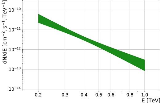
Time-averaged VHE spectrum of 1ES 2322−409 as a function of true energy. The green band corresponds to the 68 per cent confidence level provided by the maximum likelihood method for a power-law hypothesis.

Figure 2.

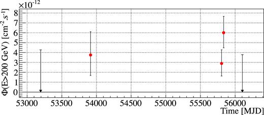
Monthly averaged integral fluxes of 1ES 2322−409 above 200 GeV. Arrows correspond to 95 per cent upper limits. Only statistical uncertainties are displayed.

3 MULTIWAVELENGTH DATA

To study the broad-band behaviour of the source, additional data were compiled over different periods and over a large spectral domain. These data, presented below, were taken from observations with Fermi LAT (100 MeV–500 GeV), RXTE PCA (2–60 keV), Swift XRT (0.2–10 keV), and Swift UVOT (170–650 nm), GROND (Sloan optical g′, r′, i′, and |$z$|′, along with infrared |$J, H, \, \mathrm{and} \, K$| filters), 2MASS (1.25, 1.65, and |$2.17\, \mu \mathrm{m}$|⁠), WISE (3.6, 4.6, 12, and |$22\, \mu \mathrm{m}$|⁠), Catalina (V band), ATOM (optical B and R filters), SUMSS (⁠|$843\, \mathrm{MHz}$|⁠), GLEAM (80–300 MHz), and TGSS (150 MHz). Only a fraction of the Fermi LAT, Swift UVOT, Swift XRT, and GROND data are quasi-simultaneous.

3.1 Fermi LAT

The LAT instrument onboard the Fermi satellite detects γ-ray photons with energies between 20 MeV and above 300 GeV. Data were analysed using the publicly available Science Tools v10r0p5.² Photons in a circular region of interest (RoI) of radius 10°, centred on the position of 1ES 2322−409, were considered. The PASS 8 instrument response functions (event class 128 and event type 3) corresponding to the P8R2_SOURCE_V6 response were used together with a zenith-angle cut of 90°. The model of the region of interest was based on the 3FGL catalogue (Acero et al. 2015). The Galactic diffuse emission has been modelled using the file gll_iem_v06.fits (Acero et al. 2016) and the isotropic background using iso_P8R2_SOURCE_V6_v06.txt.

Fermi-LAT data have been analysed for a period spanning from 2008 August 4 (MJD 54682) to 2015 July 1 (MJD 57204). Assuming a power-law spectral shape for 1ES 2322−409, as per the 3FGL model (Acero et al. 2015), a binned likelihood analysis yields a detection with a Test Statistic TS = 787 (∼28σ) with an integrated photon flux of |$F_\rm{100\,{MeV}--500\, {GeV}} = (7.17 \pm 0.97) \times 10^{-9}\, \mathrm{cm^{-2}\, s^{-1}}$| and a photon index of Γ = 1.79 ± 0.05. The fit is performed iteratively, as described in H.E.S.S. Collaboration (2013b). Using an alternative, more complex spectral model such as a log parabola does not significantly improve the fit. The most energetic photon detected from 1ES 2322−409 has an energy of ∼118 GeV at a 95 per cent confidence level, as obtained using gtsrcprob.

Because the source PKS 2325−408, whose brightness is comparable to the one of 1ES 2322−409, is close-by in the RoI, at only 0.69° from 1ES 2322−409, and considering the large point spread function of the Fermi LAT at low energies (∼5° at 100 MeV, ∼0.8° at 1 GeV and smaller than 0.1° at 500 GeV, Atwood et al. 2013), the data set was also analysed using a higher energy threshold of 1 GeV, in order to rule out leakage of photons from this nearby source. The corresponding results are compatible with the analysis performed using the full energy range, thus demonstrating that the modelling of the region of interest is under control in the entire energy range.

Data spanning from 2010 June 3 (MJD 55350) to 2011 March 30 (MJD 55650) will be used for the SED modelling (see Section 4, Fig. 6). In that time window, 1ES 2322−409 is detected with a TS of 198 (∼14σ), with an integrated photon flux |$F_{100\, \mathrm{MeV}\text{--}500\, \mathrm{GeV}} = (8.15 \pm 2.30) \times 10^{-9}\, \mathrm{cm^{-2}\, s^{-1}}$| and a photon index of Γ = 1.69 ± 0.11, and thus fully compatible with the entire data set within statistical errors.

The long-term variability pattern was tested using 1-yr time bins, with a constant fit to the light curve yielding χ²/n.d.f. = 8.58/5 (see Fig. 3). Even at shorter time scales, no variability is clearly seen in the monthly binned light curve (see Fig. 6), a fit to a constant flux yielding χ²/n.d.f. = 79.8/67 with a p-value of 0.14. This is consistent with the variability index of 41.32 reported by the Fermi-LAT collaboration in the 3FGL catalogue (Acero et al. 2015).

Figure 3.

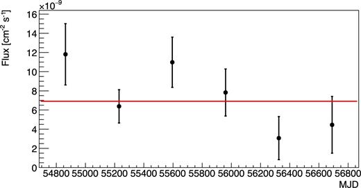
Yearly binned light curve of Fermi-LAT data, in the energy range 100 MeV to 500 GeV. The red line corresponds to a constant fit to the light curve.

3.2 RXTE PCA

X-ray observations of 1ES 2322−409 in the energy range 2–|$60\, \mathrm{keV}$| were performed with the Proportional Counter Array (PCA, Jahoda et al. 1996) onboard the RXTE spacecraft. Seven pointings were taken nightly from the 2011 December 15 to 21 for 1ES 2322−409. None of these pointings are contemporaneous with H.E.S.S. observations. The exposures of the PCA units are listed in Table 1. The analysis was performed using the standard heasoft (v6.16) and xspec (v12.9) tools. The STANDARD2 data with a time resolution of 16 s and with energy information in 128 channels were extracted and filtered following the RXTE Guest Observer Facility (GOF) recommended criteria. Data were binned to ensure a minimum of 20 counts per bin. Despite the broader energy range of the instrument, the source only presented sufficient statistics in the 3–|$7\, \mathrm{keV}$| energy range. Thus, the average photon intrinsic spectrum from of all the seven PCA observations was calculated in this energy range for a power-law function. With the column density fixed at the Galactic value, i.e. |$N_{\text{H,tot}} = 1.67\times 10^{20}\, \mathrm{cm}^{-2}$| (Willingale et al. 2013), we obtained a photon index of Γ = 2.80 ± 0.15 and a normalization at 1 keV of |$\phi _0 = (7.26^{+1.80}_{-1.43})\times 10^{-3} \, \mathrm{keV}^{-1}$| s⁻¹ cm⁻² (see Table 2 for fit parameters). The fit is not significantly improved considering a broken power-law (BPL) shape, an F-test to compare the model fits yielding a probability of 0.043.

Table 1.

Available RXTE observations, corresponding dates, and exposure times.

Date	MJD	Our ID	RXTE ID	Exp (ks)
2011-12-15 02:11:44	55910.09	OBS A	96141-01-01-00	6.3
2011-12-16 01:38:56	55911.06	OBS B	96141-01-02-00	5.94
2011-12-16 23:32:48	55911.98	OBS C	96141-01-03-00	5.41
2011-12-18 00:33:52	55913.02	OBS D	96141-01-04-00	2.34
2011-12-19 01:34:40	55914.06	OBS E	96141-01-05-00	6.54
2011-12-19 21:54:40	55914.91	OBS F	96141-01-06-00	5.68
2011-12-21 00:29:36	55916.02	OBS G	96141-01-07-00	5.68

Table 2.

De-absorbed power-law parameters describing the differential photon flux obtained with XSPEC for RXTE PCA observations (columns 2, 3, and 4), along with the 3–7 keV de-absorbed integrated energy flux (column 5). See Section 3.2 for more details.

Our ID	Photon index	Normalization at 1 keV	|$\chi ^2_{\mathrm{ red}}$| (d.o.f.)	F
		(⁠|$\rm keV^{-1} \, s^{-1} \, cm^{-2}$|⁠)		(10−12|$\rm erg \, cm^{-2}\, s^{-1}$|⁠)
TOTAL	2.80 |$_{-0.15}^{+0.15}$|	(7.26 |$_{-1.43}^{+1.80}$|⁠) × 10−3	1.13 (7)	2.93|$_{-0.86}^{+0.82}$|
OBS A	2.8	(6.56|$_{-0.49}^{+0.49}$|⁠) × 10−3	0.970 (8)	2.69|$_{-0.19}^{+0.20}$|
OBS B	2.8	(5.94|$_{-0.50}^{+0.50}$|⁠) × 10−3	0.334 (8)	2.43|$_{-0.20}^{+0.20}$|
OBS C	2.8	(7.50 |$_{-0.68}^{+0.68}$|⁠) × 10−3	0.286 (8)	3.06|$_{-0.28}^{+0.28}$|
OBS D	2.8	(1.23 |$_{-0.17}^{+0.17}$|⁠) × 10−2	0.733 (8)	5.05|$_{-0.70}^{+0.70}$|
OBS E	2.8	(9.55 |$_{-1.01}^{+1.01}$|⁠) × 10−3	0.561 (8)	3.92|$_{-0.41}^{+0.41}$|
OBS F	2.8	(7.26 |$_{-1.07}^{+1.07}$|⁠) × 10−3	0.192 (8)	2.98|$_{-0.44}^{+0.43}$|
OBS G	2.8	(6.96 |$_{-1.06}^{+1.06}$|⁠) × 10−3	0.831 (8)	2.85|$_{-0.43}^{+0.44}$|

In order to obtain the integrated flux light curve, we performed observation-by-observation analyses. To do so, because of low net count rates, we fixed the photon index of all individual observations to that of the average state, i.e. Γ = 2.80 ± 0.15. Corresponding fluxes in the 3–7 keV range along with fit results are presented in Table 2. The source showed a small flare between the December 18 and 19 (Fig. 4). The fit of a constant to the light curve indicates evidence for variability with a chance probability of |${\sim }0.1{{\ \rm per\ cent}}$|⁠.

Figure 4.

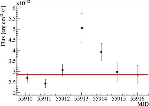
RXTE PCA light curve for all the available observations. Points correspond to the 3–|$7\, \mathrm{keV}$| de-absorbed integrated energy flux. Dates are in MJD. The red line corresponds to a constant fit to the light curve.

3.3 Swift XRT and UVOT observations

X-ray and optical/UV observations of 1ES 2322–409 were performed with the XRT and UVOT detectors onboard the Swift spacecraft (Burrows et al. 2005). The source was observed in eight different occasions between 2009 November and 2013 October (OBS 1–8, see Table 3). None of these observations are contemporaneous with H.E.S.S. data. Results of the analysis of the datasets with the most comprehensive coverage both in XRT and UVOT energy bands are presented below, since they represent the best case scenario for modelling the SED of the source. Note that OBS5 is omitted since the source is barely in the field of view and in a region with badly corrected exposure maps.

Table 3.

Available eight Swift observations, corresponding dates, IDs, and exposure times in kiloseconds.

Date	MJD	Our ID	Swift ID	Exposure (ks)
2009-11-17 13:37:00	55152.56	OBS1	00031537001	4.43
2010-03-30 06:53:00	55285.28	OBS2	00040685001	1.18
2010-03-30 08:33:00	55285.35	OBS3	00040685002	4.50
2010-10-30 05:33:00	55499.23	OBS4	00041657001	1.13
2010-10-30 10:24:01	55499.43	OBS5	00041656001	1.23
2012-11-04 02:51:00	56235.11	OBS6	00040854001	1.24
2013-10-09 18:41:29	56574.77	OBS7	00031537002	3.97
2013-10-12 00:54:00	56577.03	OBS8	00031537005	3.12

3.3.1 XRT

X-ray observations of 1ES 2322−409 were performed with the XRT detector in photon counting (PC) mode in the 0.3–10 keV energy range. Data were analysed following the standard xrtpipeline procedure³ within the heasoft (v6.16) tools and were calibrated using the last update of CALDB. Source counts were extracted with the xselect tool from a circular region of radius 30 pixels (∼71 arcsec), centred on the source, while background counts were extracted from a source-free region of radius 60 pixels. No pile-up correction was needed since the count rate was always lower than 0.5 cts s⁻¹. The spectral analysis was performed via xspec, and data were binned to ensure a minimum of 20 counts per bin. The energy range was limited for each observation to ensure an acceptable number of event statistics. In the case of the observation with the best statistics, energies ranged from 0.4 to 6.0 keV, while for the integrated fluxes featured in the light curve (Fig. 6), a common range from 0.4 to 4.0 keV was selected. Following a procedure similar to that used for the RXTE PCA data, a power law was fitted to the different XRT data sets. Table 4 gathers the best-fitting parameters derived for each individual observation considering a fixed Galactic column density (i.e. |$N_{\text{H,tot}} = 1.67\times 10^{20}\, \mathrm{cm}^{-2}$|⁠), along with the integrated fluxes.

Table 4.

De-absorbed power-law parameters describing the differential photon flux obtained with xspec for the available XRT observations, along with the 0.4–4.0 keV de-absorbed integrated energy flux featured in the light curve shown in Fig. 6. See Section 3.3.1 for more details.

Our ID	Photon index	Normalization at 1 keV	|$\chi _{\mathrm{ red}}^2$|(d.o.f.)	F
		(⁠|$\rm keV^{-1} \, s^{-1} \, cm^{-2}$|⁠)		(10−12|$\rm erg \, cm^{-2}\, s^{-1}$|⁠)
OBS1	2.35 |$_{-0.06}^{+0.05}$|	(2.32 ± 0.07) × 10−3	1.08 (52)	8.09|$_{-0.46}^{+0.46}$|
OBS2	2.30 |$_{-0.15}^{+0.15}$|	(1.13 ± 0.09) × 10−3	0.76 (8)	3.95|$_{-0.34}^{+0.24}$|
OBS3	2.42 |$_{-0.07}^{+0.06}$|	(1.51 ± 0.06) × 10−3	0.86 (35)	5.26|$_{-0.40}^{+0.40}$|
OBS4	2.14 |$_{-0.09}^{+0.09}$|	(2.59 ± 0.13) × 10−3	1.10 (21)	9.27|$_{-0.31}^{+0.31}$|
OBS6	2.67 |$_{-0.17}^{+0.17}$|	(1.01 ± 0.09) × 10−3	1.01 (7)	3.47|$_{-0.52}^{+0.52}$|
OBS7	2.36 |$_{-0.07}^{+0.07}$|	(1.27 ± 0.05) × 10−3	1.30 (25)	4.57|$_{-0.31}^{+0.33}$|
OBS8	2.43 |$_{-0.18}^{+0.19}$|	(1.17 ± 0.06) × 10−3	1.10 (15)	4.06|$_{-0.80}^{+0.81}$|

The XRT light curve (Fig. 6) illustrates variability but is not sufficiently well sampled to extract further information. A closer look at the spectral index and flux values from Table 4 reveals a ‘harder when brighter’ trend, with a correlation coefficient of −0.70. The observation with the brightest flux, OBS4, presents the hardest spectral index, Γ = 2.14 ± 0.09, closely followed by observation with the second brightest flux, OBS1 with an index of |$\Gamma = 2.35_{-0.06}^{+0.05}$|⁠. The observation with the faintest flux, OBS6, has the largest spectral index, Γ = 2.67 ± 0.17. This is also visible in Fig. 5. The modelling presented in Section 4 will focus on the high state of the source as seen by Swift in OBS4.

Figure 5.

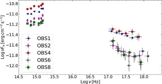
SED of different Swift UVOT (absorption corrected) and XRT observations. Red points correspond to the highest state (OBS4) that will be afterwards used for the modelling of the source’s energy distribution. Blue, magenta, red, grey, and green points correspond to OBS 1, 2, 4, 6, and 8, respectively.

3.3.2 UVOT

Simultaneous to XRT observations, the Swift UVOT telescope (Roming et al. 2005) can acquire data in six filters: |$v$|⁠, b, and u in the optical band, uw1, uvm2, and uvw2 in the ultraviolet. UVOT also features two grism modes, which provide rough spectroscopy in V and UV. For OBS3, only the uvw2 filter was available, limiting its utility. For this reason OBS3 was omitted in our analysis. Likewise, OBS7 was of grism type precluding photometric analysis, and therefore was also omitted. All available filters in each UVOT observation were searched for variability with the uvotmaghist tool. Since no variability was observed in any filter, we then summed the multiple images within each filter. Source counts were extracted from a circular region of radius 5 arcsec centred on the source. Background counts were derived from an off-source region of radius 40 arcsec. Count rates were then converted to fluxes using the standard photometric zero-points (Poole et al. 2008). The reported fluxes are de-reddened for Galactic absorption following the procedure in Roming et al. (2009), with E(B − V) = 0.0200 ± 0.0004. The source exhibited variability between different observations, reaching a maximum flux around MJD 55499 (see Tables 5 and 6 for UVOT exposure times and magnitudes for each passband, and Fig. 6 for the corresponding light curve). Fig. 5 shows the resulting UVOT photometric points, along with the previously mentioned XRT spectra.

Figure 6.

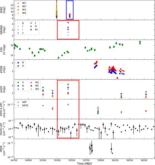
Multiwavelength light curves of 1ES 2322−409, from MJD 54750 to MJD 56700, in order of increasing energy, i.e. WISE, GROND, Catalina, ATOM, Swift UVOT (non-corrected for absorption), Swift XRT, RXTE PCA, Fermi LAT, and H.E.S.S. (from top to bottom). The red rectangle encompasses the available quasi-simultaneous data, i.e. GROND, Swift UVOT and XRT, and Fermi-LAT data, which are used for the modelling of the Swift high state of the source, while the blue rectangle shows the contemporaneous WISE data, also considered for the modelling. The GROND, Catalina, ATOM, and WISE light curves correspond to the data presented in Section 3.4. The UVOT light curves are presented in Tables 5 and 6, the XRT light curve in Table 4 and the PCA light curve in Table 2. The Fermi-LAT and H.E.S.S. light curves correspond to 28 days-averaged and weekly averaged fluxes, respectively (triangles correspond to 95 per cent upper limits). Note that a zoom into the epoch for which most MWL observations were taken has been applied, so the totality of existing H.E.S.S. data (which is considered for the modelling) is not shown in this picture (see Fig. 2 for the whole H.E.S.S. light curve). Only statistical uncertainties are displayed. Note that the high-energy light curves are shown in logarithmic scale.

Table 5.

Available UVOT photometric observations. The first column presents our observation ID, while the second states the number of individual images (extensions) within each observation. Exposure times, magnitudes, and fluxes (non-corrected for absorption) are given for different filters.

Our ID	Ext.	uvv filter (λ0 = 5402 Å)			uvb filter (λ0 = 4329 Å)			uvu filter (λ0 = 3501 Å)
		Exp	Mag	Flux	Exp	Mag	Flux	Exp	Mag	Flux
		(s)	(Vega system)	(⁠|$\rm mJy \, Hz^{-1}$|⁠)	(s)	(Vega system)	(⁠|$\rm mJy \, Hz^{-1}$|⁠)	(s)	(Vega system)	(⁠|$\rm mJy \, Hz^{-1}$|⁠)
OBS1	7	266.4	15.79 ± 0.04	1.76 ± 0.06	266.4	16.16 ± 0.03	1.39 ± 0.04	266.4	15.17 ± 0.03	1.23 ± 0.03
OBS2	1	95.2	16.09 ± 0.07	1.33 ± 0.08	95.2	16.50 ± 0.05	1.02 ± 0.04	95.2	15.51 ± 0.04	0.90 ± 0.03
OBS4	1	100.1	15.57 ± 0.05	2.15 ± 0.10	100.1	15.91 ± 0.03	1.75 ± 0.06	100.2	14.94 ± 0.03	1.52 ± 0.05
OBS6	2	–	–	–	40.2	16.62 ± 0.07	0.91 ± 0.06	40.1	15.83 ± 0.04	0.67 ± 0.04
OBS8	6	187.1	16.23 ± 0.05	1.17 ± 0.05	243.9	16.68 ± 0.03	0.86 ± 0.03	244.0	15.72 ± 0.03	0.75 ± 0.02

Table 6.

Continuation of Table 5.

Our ID	Ext.	uvw1 filter (λ0 = 2634 Å)			uvm2 filter (λ0 = 2231 Å)			uvw2 filter (λ0 = 2030 Å)
		Exp	Mag	Flux	Exp	Mag	Flux	Exp	Mag	Flux
		(s)	(Vega system)	(⁠|$\rm mJy \, Hz^{-1}$|⁠)	(s)	(Vega system)	(⁠|$\rm mJy \, Hz^{-1}$|⁠)	(s)	(Vega system)	(⁠|$\rm mJy \, Hz^{-1}$|⁠)
OBS1	7	534.2	15.04 ± 0.03	0.86 ± 0.02	555.6	14.96 ± 0.03	0.80 ± 0.02	1069.6	15.01 ± 0.02	0.73 ± 0.02
OBS2	1	190.7	15.37 ± 0.04	0.64 ± 0.02	289.8	15.29 ± 0.04	0.59 ± 0.02	381.7	15.34 ± 0.03	0.54 ± 0.01
OBS4	1	200.6	14.83 ± 0.03	1.04 ± 0.03	300.1	14.71 ± 0.03	1.00 ± 0.03	401.3	14.82 ± 0.03	0.87 ± 0.02
OBS6	2	85.6	15.75 ± 0.06	0.45 ± 0.02	120.8	15.50 ± 0.06	0.48 ± 0.03	161.2	15.80 ± 0.05	0.35 ± 0.02
OBS8	6	491.9	15.66 ± 0.03	0.49 ± 0.01	368.6	15.53 ± 0.04	0.47 ± 0.02	918.2	15.68 ± 0.03	0.40 ± 0.01

3.4 Optical and radio data

The Automatic Telescope for Optical Monitoring (ATOM) is a 75 cm telescope located on the H.E.S.S. site (Hauser et al. 2004). Data for 1ES 2322−409 in the R and B bands are scattered between MJD 55850 and MJD 56300 with a typical sampling frequency of 1 d, and are only simultaneous with H.E.S.S. observations for a brief period of time. The flux points are included in the light curve in Fig. 6. The source went into a state of increasing flux with a hint of a flare peaking between MJD 55850 and MJD 56000. A second smaller flare was also observed around MJD 56100–56150. The observed variability time-scale is shorter than the ATOM data sampling.

Data are also available from the Catalina Sky Survey (CSS,⁴ Drake et al. 2009) over the same period of time as the Fermi-LAT data sampled here. The CSS consists of 7 yr of photometry taken with the Catalina Schmidt Telescope located in Arizona (USA). Fig. 6 presents V magnitude light curve for 1ES 2322–409, which is found to be highly variable in the optical, as also observed with ATOM.

GROND (Gamma-Ray Optical/Near-infrared Detector, Greiner et al. 2008) is a 7-channel imager mounted at the MPG/ESO 2.2 m telescope in La Silla, Chile. Three infrared bands (⁠|${J} = 1.24\, \mu \mathrm{m}$|⁠, |${H} = 1.63\, \mu \mathrm{m}$|⁠, |${K}_\text{s} = 2.19\, \mu \mathrm{m}$|⁠) and the Sloan optical bands (⁠|${g}^{\prime } = 475\, \mathrm{nm}$|⁠, |${r}^{\prime } = 622\, \mathrm{nm}$|⁠, |${i}^{\prime } = 763\, \mathrm{nm}$|⁠, and |${z}^{\prime } = 905\, \mathrm{nm}$|⁠) are observed simultaneously, which is particularly interesting to analyse rapidly variable sources such as blazars. The photometric data points for our analysis were taken from Rau et al. (2012). A single observation was taken on 2010 October 31 at 23:54 (see Table 3 and the light curve in Fig. 6). Because the UVOT measurements often start earlier than ground-based measurements, some fine-tuning is required in order to compare both data sets. According to Krühler et al. (2011), the spectral overlap of UVOT and GROND can be used to correct the data between both instruments. The variability-correction factor |$\Delta _{m_{\mathrm{ GR} \rightarrow \mathrm{ UV}}}=0.3$| from Rau et al. (2012) based on the mentioned spectral overlap has been applied so that GROND points can be compared directly to the corresponding simultaneous UVOT points of OBS4.

WISE (Wide-field Infrared Survey Explorer, Wright et al. 2010) observations were considered for the SED too. WISE is an infrared-wavelength astronomical space telescope launched in 2009 December. With a 40-cm-diameter (16-in.) aperture, it was designed to continuously image broad stripes of sky at four infrared wavelengths (⁠|$3.4$|⁠, |$4.6$|⁠, |$12,$| and |$22\, \mu \mathrm{m}$|⁠) as the satellite orbits the Earth. For 1ES 2322−409, the observations were taken in two different time windows: the four filters were active during the first one (∼MJD 55340), but only two (W1 and W2) for the second one (∼MJD 55530), which is the period contemporaneous to the simultaneous GROND and Swift observations (see Fig. 6). WISE light curves were closely inspected in search of variability during this contemporaneous period. The lack of it allows us to consider the averaged spectral points for the SED.

Although not used for the SED modelling of the source because they are out of the time-window considered in this work, radio data from the Sydney University Molonglo Sky Survey (SUMSS, Mauch et al. 2003),⁵ the TIFR GMRT Sky Survey (TGSS, Intema et al. 2017) and the GaLactic and Extragalactic All-sky MWA Survey (GLEAM, Hurley-Walker et al. 2017; Wayth et al. 2015) are also available for 1ES 2322−409, and are depicted in Fig. 7.

Likewise, there are non-simultaneous Two Micron All Sky Survey (2MASS, Skrutskie et al. 2006) data, taken on 1999 August 8. Although not used for modelling purposes, we decide to show these data in the MWL SED (Fig. 7) to have a broad picture of the source’s spectrum, regardless of simultaneity constraints.

4 MODELLING AND DISCUSSION

The rich MWL dataset gathered on 1ES 2322−409 allows us to perform for the first time a detailed study of its broad-band emission from infrared to VHE. A key step before performing the SED modelling is to carefully select the data in order to avoid variability effects that can bias the reconstruction of the source parameters. In the following we build a quasi-simultaneous SED of 1ES 2322−409 and interpret it in the framework of the standard SSC model for blazar emission, which has been successful in describing the emission from γ-ray HSP blazars. Given that the redshift of the source is unknown, we perform a study for the tentative value of |$z$| = 0.17 provided by Jones et al. (2009), and then test |$z$| = 0.06, close to the redshift of several galaxies found around 1ES 2322−409 in shallow surveys⁶ (Ratcliffe et al. 1996; Shectman et al. 1996; Vettolani et al. 1998; Jones et al. 2009).

The light curves of 1ES 2322−409 at different wavelengths are presented in Fig. 6. There is no evidence of strong long-term variability observed at γ-ray energies. Day-scale and month-scale variability is seen both in optical and X-ray wavelengths. X-ray and optical/UV fluxes measured with XRT and UVOT are correlated, with a correlation coefficient higher than 0.9 whatever the UVOT filter considered.

The period around MJD 55499 is considered for further analysis, as it is the only one with a quasi-simultaneous broad-band data set including IR, optical, X-rays, and γ-rays. It corresponds to OBS4 in Swift data, which is the highest state both in optical/UV and soft X-ray wavelengths (see Fig. 5). The simultaneous GROND observations for this period of time help constrain the synchrotron component. The contemporaneous WISE observations (∼MJD 55530) are also considered for the synchrotron peak constraints, whereas the high energy bump can be defined with a subset of the Fermi-LAT data, corresponding to 300 d around MJD 55499, and the whole H.E.S.S. data set.

Since the available data set for 1ES 2322−409 (see Fig. 7) does not call for a more sophisticated approach, a one-zone stationary homogeneous synchrotron-self-Compton (SSC) model, based on Katarzyński, Sol & Kus (2001), was chosen to provide a first characterization of the parameters of the emission region. In this model, radiation is produced in a single zone of the jet approximated as a sphere of radius R, with a tangled magnetic field B, which moves through the relativistic jet at a small angle θ with respect to the line of sight. This description implies that the photons up to X-rays forming the first broad bump observed in the SED of BL Lac type blazars are produced by a population of relativistic electrons via synchrotron radiation. These synchrotron photons are then Inverse Compton (IC) scattered by the same population of electrons up to γ-ray energies, creating the second broad bump featured in the SED. The observed spectral shape requires a relativistic electron population that steepens with energy, which is conveniently modelled with a BPL with a sharp high-energy break. This approach generally provides a good overall representation of the distribution of radiating particles.

The model can be completely described with three parameters related to the global features of the emitting region, namely the magnetic field B, the radius of the region R and its bulk Doppler factor δ, and with six parameters linked to the electron energy distribution, i.e. the BPL indexes n₁ and n₂, the minimal and maximal electron energies γ_min and γ_max, the break energy γ_b and the normalization of the BPL K.

Causality implies that the flux variability time-scale t_var is related to the size of the emitting region following R ≤ ct_varδ(1 + |$z$|⁠)⁻¹, where δ is the Doppler factor and |$z$| the redshift of the source. For an estimate of this limit, we focused on modelling the flaring state of the source and applied the 1–2 d variability time-scale of the jet as seen in the X-ray band by RXTE PCA.

From the broad-band SED in Fig. 7, one can see that both the synchrotron peak and the Compton peak are well determined by observational data. A precise determination of the synchrotron peak ν_sync and its luminosity νf_ν,sync is fundamental to constrain the SSC model. Considering that the synchrotron radiation from a BPL electron distribution is well described by a smoothly BPL, we fit this function to the selected SED data, i.e. Swift high state, GROND, and WISE data (see Fig. 8), to determine the position and luminosity of the synchrotron peak. The best-fitting result is ν_sync = (2.09 ± 0.12) × 10¹⁵ Hz, and ν f_ν,sync = (1.55 ± 0.02) × 10⁻¹¹ erg cm⁻² s⁻¹. Since the SSC peak is located at approximately ν_comp ∼ 10²⁵ Hz, and the break energy γ_b of the BPL electron distribution in the Thomson regime is expected to be located at (3ν_comp/4ν_sync)^1/2 (Tavecchio, Maraschi & Ghisellini 1998), we estimate that γ_b is of the order of 10⁴.

Figure 8.

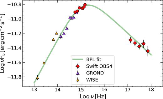
Spectral energy distribution of the source zoomed over the synchrotron-peak energy range. In green, the smoothly BPL fit of the high state XRT, UVOT, and GROND simultaneous data along with contemporaneous WISE data, which helps to determine the location of the synchrotron peak of the source.

Figure 7.

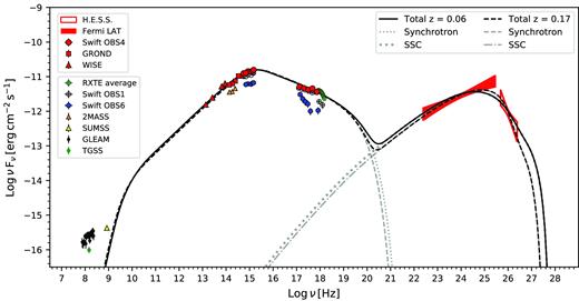
SSC modelling of the SED of 1ES 2322−409 considering two values for the redshift z = 0.17 and z  = 0.06. Red symbols correspond to data selected for the SED modelling (see Section 4 for further explanation): the red hollow and filled bow ties represent the whole H.E.S.S. and a sub-set of the Fermi-LAT data, respectively; the red circles, squares, and triangles represent the Swift OBS4, GROND, and WISE data, respectively. Available data corresponding to other periods are also shown: green circles correspond to RXTE data, black hollow and blue circles correspond to Swift OBS1 and OBS6, respectively, orange triangles to 2MASS data, yellow triangles to SUMSS data, black diamonds to GLEAM data, and green diamonds to TGSS data. Only statistical uncertainties are displayed. The dashed black line corresponds to a selected solution of the high-redshift SSC model, whereas the solid black line corresponds to a selected solution of the low-redshift SSC model. Absorption of the VHE emission by the extragalactic background light is accounted for following the model by Franceschini et al. (2008). See Table 7 for input parameters for the model.

Using the constraints on the peak positions and luminosities of the synchrotron and SSC components as starting points, the parameter space of the model was explored systematically using the algorithm developed by Cerruti, Boisson & Zech (2013). Five free parameters were investigated, in the following sub-set of the parameter space: δ ∈ [10, 100], |$B\in [2,50]\, \mathrm{mG}$|⁠, |$R\in [1\times 10^{16}, 2\times 10^{17}]\, \mathrm{cm}$|⁠, γ_b ∈ [1 × 10⁴, 1 × 10⁵], |$K\in [1\times 10^{-8}, 5\times 10^{-6}]\, \mathrm{cm}^{-3}$|⁠, where K is defined as the normalization of the electron distribution at γ_b. Solutions outside the sampled parameter space do not exist, as they are excluded analytically following the approach described in Tavecchio et al. (1998). Two assumptions of the redshift of the source were probed, using the model by Franceschini, Rodighiero & Vaccari (2008) to account for the absorption of the VHE emission by the extragalactic background light. The indices of the particle distribution n₁ and n₂, being well constrained by the Fermi-LAT and Swift XRT spectra, respectively, were fixed to values within the uncertainties of the measured slopes that provided a maximum range of acceptable model solutions. This was necessary to reduce the large number of degrees of freedom of the model considered for the parameter scan. The values of γ_min and γ_max were also fixed, given the small impact of these parameters on the model SED. Taking into account the considerations above, 12⁵ SSC models were produced, computing for each of them the frequency and flux of the synchrotron peak, the flux and spectral index in the H.E.S.S. energy band, and the flux and spectral index in the Fermi-LAT energy band. To compare with the γ-ray observables, we calculate for every SSC model a fit with a power-law function over the Fermi-LAT and H.E.S.S. detection bands, obtaining the associated dependence of the spectral index and the flux at the instrumental decorrelation energy on each model parameter. In addition to these four γ-ray observables, the two synchrotron observables introduced above are also used in the following. Each of these six observables is then expressed as a function of the model parameters, producing a set of equations. With five variables, a system of five equations is enough to provide a unique constraint on each variable. We solve the system requiring that log(ν_sync) ∈ [15.29, 15.34], log(νf_ν,sync) ∈ [−10.81, −10.80], log(νf_ν,LAT) ∈ [−11.64, −11.48], log(νf_ν,H.E.S.S.) ∈ [−12.185, −11.915], Γ_H.E.S.S. ∈ [−4.09, −2.71], where ν_sync is in Hz and νf_ν is in |$\mathrm{erg\, cm^{-2}\, s^{-1}}$|⁠. We further select solutions which satisfy the conditions on the LAT index Γ_LAT ∈ [−1.89, −1.49] and the variability time-scale |$t_{\rm var} \lt 1.5\, \mathrm{d}$|⁠. We also exclude solutions with δ > 100, which are outside the explored parameter space and much higher than estimations from radio observations. Please note that the γ-ray observables include the systematic uncertainties, summed in quadrature to the statistical ones. Note also that no χ² minimization is performed, as the algorithm simply selects SSC solutions which are compatible with the observations, as a numerical generalization of the Tavecchio et al. (1998) approach. The values of the SSC solutions are provided in Table 7. For each solution the energy budget of the emitting region is calculated, and we provide the range of derived u_e/u_B and L values, where u_e and u_B are the kinetic and magnetic energy densities in the source frame and L is the jet power.

Table 7.

SSC model parameters for |$z$| = 0.06 and |$z$| = 0.17. The values in the ‘Range’ column correspond to the allowed intervals obtained from the scan of the parameters space using the algorithm developed by Cerruti et al. (2013). The values in the ‘Example’ columns correspond to particular solutions selected for illustration purpose. See text for the definition of the different parameters.

	z  = 0.06		z  = 0.17
	Range	Example	Range	Example
δ	[15, 52]	20	[22, 100]	30
K (1/cm3)	[1.2 × 10−7, 3.7 × 10−6]	1.5 × 10−7	[0.2 × 10−7, 4.0 × 10−6]	0.3 × 10−7
R (cm)	[1.1 × 1016, 7.3 × 1016]	6.7 × 1016	[1.2 × 1016, 1.6 × 1017]	1.6 × 1017
B (mG)	[13, 49]	20	[3, 37]	10
n1	Fixed	1.7	Fixed	1.7
n2	Fixed	3.5	Fixed	3.5
γmin	Fixed	100	Fixed	100
γb	[1.8 × 104, 3.2 × 104]	3 × 104	[1.6 × 104, 4.5 × 104]	4 × 104
γmax	Fixed	5 × 106	Fixed	5 × 106
ue/ub	[5, 156]	23	[8, 536]	34
L (1043 erg s−1)	[1.5, 3.9]	3.4	[6.2, 33.4]	17.6

Given the degeneracy of the SSC model and the correlations between different parameters, an optimal solution cannot be identified, but it is instructive to discuss selected examples. The selected solutions have bulk Doppler factors δ and energy density ratios u_e/u_B close to the lower limits found from the parameter scans.

For the source redshift |$z$| = 0.17, proposed by Jones et al. (2009), a solution with commonly assumed parameters is obtained, for example, for a Doppler factor of δ = 30, a magnetic field of B = 0.01 G and a radius of R ∼ 1.6 × 10¹⁷ cm, which is close to the limit set by the variability time-scale. A reduction in the size of the emission region would require an increase of the Doppler factor. The particle energy distribution is described with γ_b = 4 × 10⁴. The index variation between the first and second slopes of the BPL does not account for a simple synchrotron cooling break, due to the need of a relatively steep slope to match the Swift XRT data. This points to the known limitation of the simple one-zone model, where acceleration, energy loss and particle escape are not explicitly modelled (Katarzyński et al. 2001). In this scenario, the emitting region is relatively far from equipartition with a value of the electron energy density to magnetic energy density ratio, u_e/u_B ∼ 34. However, such deviations are not unexpected for a source of type HSP like 1ES 2322−409 (see e.g. Cerruti et al. 2013). The parameter values of the SSC model are not different from the ones usually obtained for the other γ-ray HSP sources (see e.g. Tavecchio et al. 2010; Zhang et al. 2012), showing that 1ES 2322−409 fits within the current population of known TeV blazars.

Considering that the |$z$| = 0.17 redshift from Jones et al. (2009) is uncertain (see Section 1), it was decided to investigate whether the redshift |$z$| = 0.06 would yield solutions with more moderate model parameters, in terms of δ or equipartition factor. For an exemplary solution with small bulk Doppler factor, a value of δ = 20 was chosen, leading to a larger value of the magnetic field strength compared to the high-redshift solution. The chosen set of parameters yields an electron and magnetic energy density ratio of u_e/u_B ∼ 23, a bit closer to equipartition than for the solution at higher redshift.

We note that the overall model does not account for the low-energy non-simultaneous radio data, which can in turn be ascribed to different larger regions of the jet. From the parameter ranges it can be seen that the SSC solutions for the lower redshift assumption (⁠|$z$| = 0.06) are concentrated in a narrower domain in parameter space than the solutions for |$z$| = 0.17. For the lower redshift, solutions can be found closer to equipartition and with more modest values of the bulk Doppler factor. Apart from these indications, no preference can be given to one or the other of the redshift estimates, based on the SSC model. It should be clear, however, that the scenario will require more extreme values if one assumed an even higher redshift for this source.

5 CONCLUSIONS

We report the discovery with the H.E.S.S. telescopes of VHE γ-ray emission from the HSP 1ES 2322−409. The source was detected at 6σ level in 22.3 h (live-time) with an average VHE γ-ray spectrum well described with a power law with a photon index Γ = 3.40 ± 0.66_stat ± 0.20_sys and an integral flux above |$200\, \mathrm{GeV}$| corresponding to 1.1|${{\ \rm per\ cent}}$| of the Crab nebula flux. We report also the analysis of multiwavelength data obtained at different times with Swift UVOT & XRT, RXTE PCA, Fermi-LAT, and additional data from WISE, GROND, Catalina, and ATOM. Swift observed the source in different states of activity. For the state corresponding to the higher Swift XRT flux, the source was quasi-simultaneously observed in the optical regime with GROND. These observations, along with contemporaneous infrared WISE data and the ∼1−2 d variability observed by RXTE, provide strong constraints for the description of the emission of the source in terms of synchrotron radiation. Using the whole H.E.S.S. data as an indicator of the source behaviour in the VHE γ-ray regime, together with Fermi-LAT data around the Swift high state, and considering two possible values |$z$| = 0.17 and |$z$| = 0.06 for the redshift of the source, we showed that a simple one-zone leptonic SSC model provides a good description of the broad-band emission of 1ES 2322−409, with parameters compatible with the ones usually obtained for the other known TeV blazars. The lack of a firm redshift is however an issue for the understanding of the source. In the absence of detection of spectral lines in the optical regime, constraints on the redshift could be provided by deeper TeV observations resulting in a significant detection at energies at or above 1 TeV, where the effects of EBL absorption will significantly differ between redshift assumptions (see e.g. Mazin & Goebel 2007).

ACKNOWLEDGEMENTS

The support of the Namibian authorities and of the University of Namibia in facilitating the construction and operation of H.E.S.S. is gratefully acknowledged, as is the support by the German Ministry for Education and Research (BMBF), the Max Planck Society, the German Research Foundation (DFG), the Alexander von Humboldt Foundation, the Deutsche Forschungsgemeinschaft, the French Ministry for Research, the CNRS-IN2P3 and the Astroparticle Interdisciplinary Programme of the CNRS, the U.K. Science and Technology Facilities Council (STFC), the IPNP of the Charles University, the Czech Science Foundation, the Polish National Science Centre, the South African Department of Science and Technology and National Research Foundation, the University of Namibia, the National Commission on Research, Science & Technology of Namibia (NCRST), the Innsbruck University, the Austrian Science Fund (FWF), and the Austrian Federal Ministry for Science, Research and Economy, the University of Adelaide and the Australian Research Council, the Japan Society for the Promotion of Science and by the University of Amsterdam. We appreciate the excellent work of the technical support staff in Berlin, Durham, Hamburg, Heidelberg, Palaiseau, Paris, Saclay, and in Namibia in the construction and operation of the equipment. This work benefited from services provided by the H.E.S.S. Virtual Organisation, supported by the national resource providers of the EGI Federation.

This research has made use of the SIMBAD database, operated at CDS, Strasbourg, France.

This publication makes use of data products from the Two Micron All Sky Survey, which is a joint project of the University of Massachusetts and the Infrared Processing and Analysis Center/California Institute of Technology, funded by the National Aeronautics and Space Administration and the National Science Foundation.

This research has made use of the NASA/IPAC Infrared Science Archive, which is operated by the Jet Propulsion Laboratory, California Institute of Technology, under contract with the National Aeronautics and Space Administration.

The CSS survey is funded by the National Aeronautics and Space Administration under Grant No. NNG05GF22G issued through the Science Mission Directorate Near-Earth Objects Observations Program. The CRTS survey is supported by the U.S. National Science Foundation under grants AST-0909182 and AST-1313422.

This research has made use of data and/or software provided by the High Energy Astrophysics Science Archive Research Center (HEASARC), which is a service of the Astrophysics Science Division at NASA/GSFC and the High Energy Astrophysics Division of the Smithsonian Astrophysical Observatory.

Co-author MA is supported by the Paris Science et Lettres (PSL) foundation. RCGC is funded by EU FP7 Marie Curie, grant agreement No. PIEF-GA-2012-332350.

Footnotes

1

https://www.mpi-hd.mpg.de/hfm/HESS/

2

See http://fermi.gsfc.nasa.gov/ssc/data/analysis/documentation.

3

http://www.swift.ac.uk/analysis/xrt/

4

http://nesssi.cacr.caltech.edu/DataRelease/

5

According to the ASDC, between 1997 and 2003.

6

Note that the lack of deep redshift surveys around the source renders a quantification whether 1ES 2322−409 is part of a group of galaxies impossible.

Author notes

Deceased.

Present address: Instituto de Física de São Carlos, Universidade de São Paulo, Av. Trabalhador São-carlense, 400 – CEP 13566-590, São Carlos, SP, Brazil.