The winds of young Solar-type stars in Coma Berenices and Hercules-Lyra

ABSTRACT

We present wind models of 10 young Solar-type stars in the Hercules-Lyra association and the Coma Berenices cluster aged around ∼0.26 and ∼0.58 Gyr, respectively. Combined with five previously modelled stars in the Hyades cluster, aged ∼0.63 Gyr, we obtain a large atlas of 15 observationally based wind models. We find varied geometries, multi-armed structures in the equatorial plane, and a greater spread in quantities such as the angular momentum loss. In our models, we infer variation of a factor of ∼6 in wind angular momentum loss |$\dot{J}$| and a factor of ∼2 in wind mass-loss |$\dot{M}$| based on magnetic field geometry differences when adjusting for the unsigned surface magnetic flux. We observe a large variation factor of ∼4 in wind pressure for an Earth-like planet; we attribute this to variations in the ‘magnetic inclination’ of the magnetic dipole axis with respect to the stellar axis of rotation. Within our models, we observe a tight correlation between unsigned open magnetic flux and angular momentum loss. To account for possible underreporting of the observed magnetic field strength we investigate a second series of wind models where the magnetic field has been scaled by a factor of 5. This gives |$\dot{M}\propto B^{0.4}$| and |$\dot{J}\propto B^{1.0}$| as a result of pure magnetic scaling.

stars: magnetic field, stars: rotation, stars: solar-type, stars: winds, outflows, Sun: evolution, Sun: heliosphere

1 INTRODUCTION

The age span linking the end of the stellar contractive phase and the onset of the Skumanich (1972) relationship P_rot∝t^1/2 between stellar period of rotation and stellar age extends from approximately 0.1–0.6 Gyr for Solar-type stars (Gallet & Bouvier 2013, 2015). Stars enter this ‘pre-Skumanich spin-down phase’ with a wide range of rotation periods (Edwards et al. 1993) depending on the specifics of the preceding contractive phase. For the Skumanich relationship to take hold at 0.6 Gyr, rapidly rotating stars must shed angular momentum more efficiently than slowly rotating stars.

Barnes (2003) found a bimodal period distribution of ‘fast and slow rotators’ in the pre-Skumanich spin-down phase and suggested that the bimodal distribution of rotation periods arise as the ‘magnetically saturated’ fast rotators are unable to effectively shed angular momentum (MacGregor & Brenner 1991) by the wind mechanisms that apply in the slow rotator group. Many models of stellar spin-down (Kawaler 1988; Bouvier 1991; Chaboyer, Demarque & Pinsonneault 1995) thus invoke a threshold rotation velocity and/or magnetic field above which angular momentum shedding is inhibited in order to permit spin braking laws to reproduce the Skumanich relationship past 0.6 Gyr. Depending on the choice of model the threshold rotation velocity can be 3–15 times the Solar rotational velocity (Matt et al. 2015; Amard et al. 2016).

The dominant mechanism of stellar spin-down is angular momentum shedding by means of the coupling between the stellar wind and the magnetic field (Schatzman 1962; Weber & Davis 1967) and the resulting magnetic and dynamic torque components acting on the star. Thus, mathematical descriptions of the stellar wind angular momentum loss |$\dot{J}$| and its history must reproduce the Skumanich relationship from a wide range of initial periods of rotation in order to agree with observations. The effect of the star’s magnetic field on the wind angular momentum loss is well known: the angular momentum loss is increased as if the magnetic field holds the escaping wind matter in co-rotation with the star until the wind speed exceeds the Alfvén wave speed |$u_\rm {\small A}$| (Alfvén 1942), thus greatly increasing |$\dot{J}$|⁠. The Alfvén radius |$R_\rm {\small A}$| at which the wind speed exceeds |$u_\rm {\small A}$| varies with the magnetic field strength, wind density, and wind velocity.

The importance of the Alfvén radius and the magnetic field geometry is seen in one-dimensional and two-dimensional solar and stellar wind models (Weber & Davis 1967; Mestel 1968, 1984; Kawaler 1988) in forms such as |$\dot{J} \propto P_\text{rot}^{-1} \dot{M} R_\rm {\small A}^n$|⁠, where n is magnetic geometry parameter. The dependence of these models on the wind mass-loss |$\dot{M}$| can limit their usefulness as |$\dot{M}$| is itself notoriously difficult to constrain observationally, and there is much uncertainty about the behaviour of |$\dot{M}$| for stars younger than ∼0.6 Gyr (Wood et al. 2005, 2014).

Numerical simulations permit the simultaneous reconstruction of |$\dot{M}$| and |$\dot{J}$| by solving the magnetohydrodynamic (MHD) equations; this, however, requires a model of the stellar surface magnetic field, and setting a coronal temperature (e.g. Vidotto 2009; Cohen & Drake 2014; Ó Fionnagáin & Vidotto 2018) and/or prescribing a model of coronal heating (van der Holst et al. 2014). Depending on the models used, other parameters may need to be estimated; these may include the magnetic filling factor (Suzuki 2011), the Poynting flux (Boro Saikia et al. 2020), the wave turbulence (Chandran et al. 2011; Cranmer et al. 2015), as well as other parameters.

As the stellar rotational energy ultimately sustains stellar magnetic fields, a greater variation in the relation between age, period of rotation, stellar magnetic fields, and stellar winds may be expected in the pre-Skumanich spin-down phase, with its range of rotation periods and differing states of magnetic saturation, than in later phases of a star’s lifespan. Depending on the saturation mechanism, on could also expect a greater variation in the relation between the surface magnetic field strength and wind mass- and angular momentum loss, for example if there is an physical increase in field complexity for more rapidly rotating stars (Garraffo et al. 2018).

In this work, we study the pre-Skumanich spin-down phase stellar winds by creating wind models of young, Solar-type stars in the Coma Berenices cluster and the Hercules-Lyra association with well characterized ages of 584 ± 10 and 257 ± 46 Myr, respectively (Folsom et al. 2018); these stars are in the late and middle pre-Skumanich spin-down phase. The Coma Berenices stars in our sample are slow rotators for their age, at and below the 25th percentile in the fast-, medium-, and slow rotator classification of Gallet & Bouvier (2013). The Hercules-Lyra stars of our sample exhibit some more variation and would be classified as slow to medium rotators for their age, sitting mostly below the 50th percentile. Depending on the saturation threshold angular velocity Ω = 2π/P_rot, some of the sample stars may be in the unsaturated regime where the shedding of angular momentum is inhibited.

The wind models presented here are based on surface magnetic maps by Folsom et al. (2016), Folsom et al. (2018), hereafter F16, F18. The lack of rotational symmetry of the stars’ surface magnetic fields, in particular the offset between the magnetic dipole axis and the stellar rotation axis mandate the use of three-dimensional numerical simulations. We use the F16, F18 magnetic maps to drive the numerical Alfvén wave Solar model (awsom; Sokolov et al. 2013; van der Holst et al. 2014), which is part of the Space weather modelling framework (swmf; Powell et al. 1999; Tóth et al. 2012). In the awsom model, the corona is heated by Alfvén waves, which are thought to originate in the stellar interior. With its inner boundary in the chromosphere, awsom incorporates the transition region, corona, and inner astrosphere; an Alfvén wave energy flux is prescribed at the model’s inner boundary. In addition to the regular magnetohydrodynamical quantities, the wind maps give the electron-, ion-, and Alfvén wave pressure at each point in the solution. From the wind maps, we calculate the steady-state wind mass-loss and angular momentum loss, the wind pressure and spatial variation of the wind pressure for an Earth-like planet,¹ and other relevant quantities in a self-consistent manner.

By combining the wind models presented in this work with the wind models of young Solar-type stars from our previous work Evensberget et al. (2021) on the 625 ± 50 Myr old Hyades cluster, hereafter Paper I, we obtain an ‘atlas’ of stellar wind models from which we are able to formulate scaling relations between aggregate quantities and the surface magnetic field strength and surface magnetic flux.

The rest of this paper is outlined as follows. In Section 2, we describe the surface magnetic maps and how they are obtained using Zeeman-Doppler imaging; in Section 3, we describe the model equations and numerical model; in Section 4, we give an overview of our model results including aggregate quantities calculated from the wind models such as mass-loss; in Section 5, we examine trends in aggregate quantities within our own data set; in Section 6, we conclude and summarize our findings.

2 OBSERVATIONS

In this work, we use stellar surface magnetic field maps based on spectropolarimetric observations of the Hercules-Lyra association made with the Narval instrument (Aurière 2003) at the Télescope Bernard Lyot, and of the Coma Berenices cluster made with the ESPaDOnS instrument (Donati 2003; Silvester et al. 2012) at the Canada–Hawaii–France Telescope. Both sets of observations were part of the ‘TOwards Understanding the sPIn Evolution of Stars’ (TOUPIES) project²; the ESPaDOnS observations were also part of the History of the Magnetic Sun Large Program at the CFHT. The reduced spectra associated with TOUPIES are available from the Polarbase (Donati et al. 1997; Petit et al. 2014) website.³

During the observations the instruments recorded the Stokes V and Stokes I circular polarization spectrum and total intensity spectrum over a period of a few weeks. The time period minimizes actual variations in the stellar magnetic field and provides sufficient phase coverage to map the entire visible surface. The stellar magnetograms that were produced from these observations are published in F16 and F18; we refer the readers to these papers for a detailed description of the observations. Table 1 gives the stars’ fundamental parameters, and Fig. 1 shows the radial magnetic field components of the magnetograms.

Figure 1.

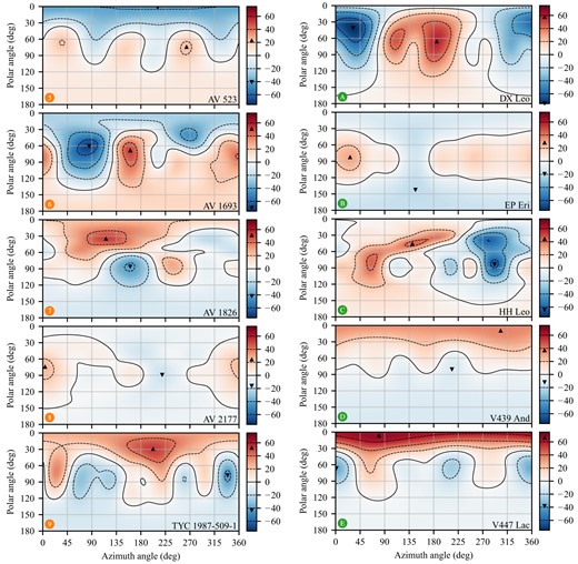
Radial magnetic field strength in Gauss for the stars modelled in this work based on the radial magnetic field coefficients derived in F16 and F18. The polar angle is measured from the rotational north pole, while the azimuth angle is measured around the stellar equator. The smallest scale of representable features is 12^○ as described in Section 2.1. The fully drawn contour line indicates a zero value of radial magnetic field strength, and the dashed contour lines represent increments as shown in the corresponding colour bar on the right of each plot. The upwards-pointing and downwards-pointing black triangles show the position and value of the maximum and minimum radial field strength values; they also appear in the colour bars so that the range of values may be easily discerned.

Table 1.

Fundamental parameters of the 10 stars modelled in this study from F16, F18, and references therein. The stellar period of rotation P_rot, radius R, and mass M are used in the magnetohydrodynamic simulations, along with the associated surface magnetic maps in Fig. 1. In the radius and mass columns, the values are scaled to the Solar values of mass |$\mathrm{M}_\odot =1.99 \times 10^{30}{\, \mathrm{kg}}$| and radius |$\mathrm{R}_\odot =6.96 \times 10^{8}\, \mathrm{m}$|⁠. In this paper, we abbreviate the full star names to the simulation case names given in the first column of this table. To aid the reader, each case name is prepended by a unique identifier symbol used throughout this paper.

Case name	Full name (see F16, F18)	Association	Type	Prot	Age	R	M	Reference
				(d)	(Myr)	(R⊙)	(M⊙)
AV 523	Cl* Melotte 111 AV 523	Coma Berenices	K2	11.10 ± 0.20	584 ± 10	0.72 ± 0.033	0.80 ± 0.05	F18
AV 1693	Cl* Melotte 111 AV 1693	Coma Berenices	G8	9.05 ± 0.10	584 ± 10	0.83 ± 0.030	0.90 ± 0.05	F18
AV 1826	Cl* Melotte 111 AV 1826	Coma Berenices	G9	9.34 ± 0.15	584 ± 10	0.80 ± 0.041	0.85 ± 0.04	F18
AV 2177	Cl* Melotte 111 AV 2177	Coma Berenices	G6	8.98 ± 0.12	584 ± 10	0.78 ± 0.033	0.90 ± 0.04	F18
TYC 1987	TYC 1987-509-1	Coma Berenices	G7	9.43 ± 0.10	584 ± 10	0.83 ± 0.033	0.90 ± 0.05	F18
DX Leo	DX Leo	Hercules-Lyra	G9	5.38 ± 0.07	257 ± 46	0.81 ± 0.026	0.90 ± 0.04	F16
EP Eri	EP Eri	Hercules-Lyra	K1	6.76 ± 0.20	257 ± 46	0.72 ± 0.081	0.85 ± 0.05	F18
HH Leo	HH Leo	Hercules-Lyra	G8	5.92 ± 0.02	257 ± 46	0.84 ± 0.030	0.95 ± 0.05	F18
V439 And	V439 And	Hercules-Lyra	K0	6.23 ± 0.01	257 ± 46	0.92 ± 0.099	0.95 ± 0.05	F16
V447 Lac	V447 Lac	Hercules-Lyra	K1	4.43 ± 0.05	257 ± 46	0.81 ± 0.089	0.90 ± 0.04	F16

In Section 5, we also include our previous Solar and Hyades cluster wind models from Paper I; the magnetograms used to drive those models were published in F18.

2.1 Magnetic mapping with Zeeman-Doppler imaging

Zeeman-Doppler imaging (ZDI; Semel 1989) has been used successfully to image the large-scale surface magnetic field of cool stars, see the review by Donati & Landstreet (2009). By using least square deconvolution (LSD; Donati et al. 1997; Kochukhov, Makaganiuk & Piskunov 2010) individual circularly polarised spectral lines are combined into a single LSD profile with a high signal-to-noise ratio.

In modern ZDI, the observable surface magnetic field is decomposed into a set of spherical harmonic coefficients (Jardine et al. 1999; Donati et al. 2006). The coefficients are found by applying the maximum entropy image reconstruction (Skilling & Bryan 1984) method to the LSD profile. In this way, a set of coefficients is found that satisfies a χ² bound on the fit while maximizing an entropy measure; we direct the reader to F16 and F18 for a detailed description of this process, which recovers all three vector components of the surface magnetic field. This work only makes use of the radial field components as is common in MHD wind modelling (see Section 3.2). The stellar surface radial magnetic field is represented as the real part of an orthogonal sum of the form

$$\begin{equation*} B_r(\theta , \varphi) = \sum _{\ell =1}^{\ell _\text{max}} \, \sum _{m=0}^\ell \alpha _{\ell m} \sqrt{\frac{2\ell +1}{4\pi } \frac{(\ell -m)!}{(\ell +m)!}} P_{\ell m}(\cos \theta) {\rm e}^{i m\varphi }, \end{equation*} $$

(1)

where α_ℓm are the complex-valued spherical harmonics coefficients of the radial field, P_ℓm(cos θ) is the associated Legendre polynomial of order m and degree ℓ, and θ, φ are the polar and azimuthal angles which identify points on the stellar surface. Since only the real part of equation (1) is of interest negative m values are omitted from the sum.⁴

The smallest features that can be reproduced by equation (1) are ∼180^○/ℓ_max in angular diameter; the magnetograms in this work use ℓ_max = 15 so that the smallest representable feature scale is ∼12^○. The ‘effective’ degree ℓ_eff can however be significantly lower than ℓ_max, resulting in only large scale features being present in the ZDI magnetograms. The effective degree depends on observational parameters such as the unpolarized line width, the star’s projected rotational velocity vsin i, and the observations’ signal-to-noise ratio (Donati & Brown 1997; Morin et al. 2010). We estimate the effective degree, ℓ_.90 and ℓ_.99, as the value of ℓ, where 90 per cent and 99 per cent of the magnetic field energy is stored in degrees lower than or equal to ℓ; the resulting values are given in Table 2, where we see values from 2 to 5 for ℓ_.90 and values from 4 to 8 for ℓ_.99. Note that the surface magnetic field values in Table 2 are calculated from the steady state magnetic field in our model output and as such they do not directly correspond to the magnetic averages in F16, F18. This is because the perpendicular components of the surface magnetic field are free to settle and converge with the numerical solution (see Section 3.2) instead of being held at their ZDI-derived values, which partly originate from photospheric currents. The ℓ_.90 and ℓ_.99 values do still give a good indication of the magnetic field complexity in a single parameter.

Table 2.

Aggregate surface magnetic field values. |B_r| and max |B_r| are the surface average and maximum absolute radial field values in Fig. 1, i.e. the average value of |B_r(θ, φ)| over the stellar surface, and the maximum value of |B_r(θ, φ)| over the stellar surface. The location (θ_max, φ_max) of max |B_r| on the stellar surface can be seen in Fig. 1. |$|\boldsymbol{B}|$| is the average surface field strength of the final steady-state solution, i.e. the average of |$|\boldsymbol{B}(\theta , \varphi)|$| over the stellar surface. ‘Dip.’, ‘Quad.’, ‘Oct.’, and ‘16+’ are the final fraction of magnetic energy in dipolar (ℓ = 1), quadrupolar (ℓ = 2), octupolar (ℓ = 3), and hexadecapolar and higher (ℓ ≥ 4) modes. The ℓ_.90 and ℓ_.99 columns refer to the magnetogram degree at which 90 per cent and 99 per cent of the magnetogram energy is contained in degrees lower than or equal to the tabulated value. Note that the tabulated |$|\boldsymbol{B}|$| values and percentages do not correspondence directly with the photospheric values in F16 and F18.

Case	|Br|	max |Br|	|$|\boldsymbol{B}|$|	Dip.	Quad.	Oct.	16+	ℓ.90	ℓ.99
	(G)	(G)	(G)	(per cent	(per cent)	(per cent)	(per cent)
AV 523	10.1	36.8	14.6	35.3	19.5	33.6	11.6	4	4
AV 1693	20.4	68.4	29.0	32.7	46.9	14.8	5.6	3	6
AV 1826	12.6	49.3	18.6	27.1	39.9	24.2	8.8	3	7
AV 2177	5.5	23.7	8.7	54.1	24.9	7.5	13.5	4	6
TYC 1987	14.7	51.4	21.4	35.1	24.2	13.3	27.4	5	5
5 ×AV 523	50.3	183.8	71.5	35.6	19.7	33.3	11.4	4	4
5 ×AV 1693	102.0	341.8	143.6	32.9	46.8	14.8	5.6	3	6
5 ×AV 1826	63.0	246.3	91.2	27.3	39.7	24.3	8.7	3	7
5 ×AV 2177	27.5	118.3	40.6	54.6	24.4	7.8	13.3	4	6
5 ×TYC 1987	73.3	256.8	105.3	35.3	24.2	13.4	27.1	5	5
DX Leo	21.1	73.2	30.0	67.1	18.1	5.8	9.0	3	5
EP Eri	9.5	27.6	14.2	29.4	63.2	0.9	6.5	2	5
HH Leo	15.3	62.4	23.0	52.2	20.7	7.8	19.4	4	8
V439 And	8.7	35.2	12.7	73.8	14.4	5.8	6.0	3	5
V447 Lac	10.4	60.7	15.7	19.5	39.3	28.0	13.3	4	5
5 ×DX Leo	105.2	366.1	148.1	66.7	18.6	5.7	9.1	3	5
5 ×EP Eri	47.5	137.8	68.6	29.9	62.7	0.9	6.5	2	5
5 ×HH Leo	76.7	311.9	112.9	52.2	20.8	7.7	19.4	4	8
5 ×V439 And	43.7	175.7	61.7	73.8	14.2	6.2	5.9	3	5
5 ×V447 Lac	51.7	303.2	76.3	19.3	39.3	28.0	13.4	4	5

While the ZDI method does not provide uncertainty estimates along with the magnetic maps, it is accepted that ZDI is able to reproduce the structure of the large-scale magnetic field. This is supported by the study of Hussain et al. (2000), which found similar results using different ZDI implementations. Polarity reversals have been observed for the stars τ Boötis (Donati et al. 2008; Fares et al. 2009, 2013; Mengel et al. 2016) and HD 75332 (Brown et al. 2021). Evidence of field reversals in HD 78366 and HD 190771 was found by Morgenthaler et al. (2011); the authors also found evidence of a more complex cycle in ξ Boötis A. Different ZDI implementations do not always agree on details of the medium- and small-scale magnetic field as noted in the review of Kochukhov (2016); however, it is the large-scale field that shapes the coronal magnetic field.

3 SIMULATIONS

In this section, we provide an overview of the numerical simulations carried out as part of this work.

3.1 Model equations

We use the Alfvén Wave Solar Model (awsom; Sokolov et al. 2013; van der Holst et al. 2014) of the Space Weather Modelling Framework (swmf; Tóth et al. 2005, 2012) to produce wind models driven by the radial component of the TOUPIES magnetic maps as described in Section 2.1. The awsom model is built upon the bats-r-us model (Powell et al. 1999; Tóth et al. 2012). An overview of awsom is found in the review of Gombosi et al. (2018).

Alfvén waves are a mechanism of coronal heating (Barnes 1968) that has been thought to contain enough energy (Coleman 1968) to power the Solar wind. In the awsom model, the wind is heated to coronal temperatures by Alfvén wave energy originating in deeper stellar layers; this is modelled as a Poynting flux |$\Pi _\rm {\small A}$| proportional to the local |$|\boldsymbol{B}|$| value at the inner model boundary. The two-temperature MHD equations are thus extended to model the propagation and dissipation of Alfvén wave energy.

We briefly state the set of differential equations solved by awsom; for a detailed description including the cooling and heating terms we refer the reader to Paper I. Mass conservation is given by

$$\begin{equation*} \frac{\partial \rho }{\partial t} + \nabla \left(\rho \boldsymbol{u}\right) = 0, \end{equation*} $$

(2a)

where ρ is the mass density and |$\boldsymbol{u}$| is the flow velocity. The induction equation is

$$\begin{equation*} \frac{\partial \boldsymbol{B}}{\partial t} + \nabla \left(\boldsymbol{u}\boldsymbol{B} - \boldsymbol{B}\boldsymbol{u}\right) = 0, \end{equation*} $$

(2b)

where |$\boldsymbol{B}$| is the magnetic field. The time evolution of Alfvén wave energy density in parallel (w⁺) and antiparallel (w⁻) directions along the magnetic field is described by

$$\begin{equation*} \frac{\partial w^\pm }{\partial t} + \nabla \left((\boldsymbol{u} \pm \boldsymbol{v}_\rm {\small A}) w^\pm \right) + \frac{w^\pm }{2}\left(\nabla \cdot \boldsymbol{u}\right) = \mp R \sqrt{w^{-} w^+} - Q^\pm _{\rm {\small W}} \end{equation*} $$

(2c)

where |$\boldsymbol{v}_\rm {\small A}= \boldsymbol{B}/\sqrt{\mu _0 \rho }$| is the Alfvén velocity, |$\mp R \sqrt{w^{-} w^+}$| are reflection rates that transfer energy between w⁺ and w⁻, and |$Q^\pm _{\rm {\small W}}$| is a dissipation term. Momentum conservation is given by

$$\begin{equation*} \frac{\partial \left(\rho \boldsymbol{u}\right)}{\partial t} + \nabla \left(\rho \boldsymbol{u}\boldsymbol{u} - \frac{\boldsymbol{B}\boldsymbol{B}}{\mu _0} + P + \frac{B^2}{2\mu _0} + P_\rm {\small A}\right) = -\rho \frac{GM \boldsymbol{r}}{r^3}, \end{equation*} $$

(2d)

where P = P_i + P_e is the sum of the ion and electron thermal pressure and |$P_\rm {\small A} = \left(w^+ + w^-\right)\big/2$| is the Alfvén wave pressure. The constants G and μ₀ are the gravitational constant and the vacuum permeability, M is the stellar mass, and |$\boldsymbol{r}$| is the positional vector (relative to the stellar centre). The ion energy equation is

$$\begin{equation*} \frac{\dfrac{\partial P_\text{i}}{\partial t} + \nabla \left(P_\text{i}\boldsymbol{u}\right) }{\left(\gamma -1\right) } + P_\text{i}\nabla \boldsymbol{u} = \frac{P_\text{e}-P_\text{i}}{\tau _\text{eq}} + f_\text{i} Q_\rm {\small W}- \rho \frac{GM \boldsymbol{r} \cdot \boldsymbol{u} }{r^3}, \end{equation*} $$

(2e)

and the electron pressure equation is

$$\begin{equation*} \frac{\dfrac{\partial P_\text{e}}{\partial t} + \nabla \left(P_\text{e}\boldsymbol{u}\right)}{\gamma -1} + P_\text{e}\nabla \boldsymbol{u} = \frac{P_\text{i}-P_\text{e}}{\tau _\text{eq}} + f_\text{e}Q_\rm {\small W}-Q_\text{rad} -\nabla \boldsymbol{q}_\text{e}, \end{equation*} $$

(2f)

with γ = 5/3 being the ratio of specific heats for monatomic gases. The right-hand side terms are collisional energy transfer ±(P_i − P_e)/τ_eq; ion/electron heating by Alfvén wave dissipation |$f_\text{i}Q_\rm {\small W}$| and|$f_\text{e}Q_\rm {\small W}$| where f_i + f_e = 1; work against gravity |$\rho G M \boldsymbol{r} \cdot \boldsymbol{u} / r^3$|⁠; radiative losses Q_rad; and electron heat conduction |$\nabla \boldsymbol{q}_\text{e}$|⁠. Paper I gives detailed descriptions of these terms.

3.2 Numerical model and boundary conditions

The model domain comprises two partially overlapping regions. The inner region uses a spherical grid and the outer region uses a Cartesian grid. The mesh is selectively refined near the stellar surface and the current sheet region where the sign of B_r changes. By stepping forward in time a steady state is reached, where the magnetic and hydrodynamic forces are in balance.

As was done in Paper I, we attempt to control for the uncertainty associated with the surface magnetic field strength measured by ZDI, we conduct two series of simulations denoted B_ZDI and 5B_ZDI. The two series of models are identical, except that the surface radial magnetic field strength is increased by a factor of 5 in the 5B_ZDI series. As the octree-based grid refinement occurs near the current sheet, the refined grid may be slightly different between the B_ZDI and 5B_ZDI case when the position of the current sheet itself is differing between the cases; we do not expect this to have any influence on the model results. The case names of each individual model in the B_ZDI series is given in Table 1; these names are used throughout this paper to identify the individual models. In the B_ZDI series the models are denoted as e.g. ‘ AV 2177’; a numbered circle and a short form of the star name. The corresponding model in the 5B_ZDI is denoted as ‘ 5 ×AV 2177’; a numbered star and 5 × followed by the star’s case name.

We use the same model parameters as in Paper I. The temperature and number density at the chromospheric inner boundary is set to Solar values |$T = 5 \times 10^{4}\, \mathrm{K}$| and |$n=2 \times 10^{17}{\, \mathrm{m}^{-3}}$| similarly to Alvarado-Gómez et al. (2016a) for example. The outgoing Alfvén wave energy density at the inner boundary is set to |$w = (\Pi _\rm {\small A}/B)_\odot \sqrt{\mu _0 \rho }$| (van der Holst et al. 2014). The value |$(\Pi _\rm {\small A}/B)_\odot =1.1 \times 10^{6}\, \mathrm{W\, m^{-2}\, m\, T^{-1}}$| (Gombosi et al. 2018) is calibrated so that awsom reproduces Solar wind conditions. A corrective scaling |$(\Pi _\rm {\small A}/B) = (\Pi _\rm {\small A}/B)_\odot (\mathrm{R/R}_\odot)^{0.3}$| as suggested by Sokolov et al. (2013) has previously been employed by Garraffo, Drake & Cohen (2016) and Dong et al. (2018) in M-dwarf wind modelling (see also Vidotto 2021). That corrective scaling is not applied as it would change the value of |$(\Pi _\rm {\small A}/B)$| by less than 10 per cent for the stellar radii in this study; we find that the two smallest R stars AV 523 and DX Leo give wind mass-loss values of ∼80 per cent of their unscaled values and similar or lower variation for the other parameters of interest.

Recently, it has been shown that wind mass-loss |$\dot{M}$| is roughly proportional to |$\Pi _\rm {\small A}/B$| (Boro Saikia et al. 2020) for Solar wind models, and some authors such as Airapetian et al. (2021) have applied large scalings to the parameter when modelling young, Solar-type stars. We briefly return to this issue and its implications in Section 6.

The radial component of the boundary magnetic field is fixed to the local magnetogram value in Fig. 1, i.e. |$\boldsymbol{B}_{\mathrm{ZDI}}\cdot \boldsymbol{\hat{r}}$| or |$5\boldsymbol{B}_{\mathrm{ZDI}}\cdot \boldsymbol{\hat{r}}$|⁠, depending on the model series. The non-radial surface magnetic field |$\boldsymbol{B}_\perp$| is part of the steady state solution inside the model domain.

4 RESULTS

In this section, we give an overview of the features in each wind model, focusing on the coronal magnetic field structure in Section 4.1; the Alfvén surface and wind speed in Section 4.2; the wind mass-loss and angular momentum loss in Section 4.3; and the wind pressure in Section 4.4. Having the full three-dimensional wind solutions make it possible to calculate a large range of wind-related quantities, including wind mass-loss, angular momentum loss, and wind pressure for an Earth-like planet. These parameters and others are presented in Table 3.

Table 3.

Aggregate wind quantities calculated from the wind models in Figs 2–4. The unsigned surface magnetic flux Φ = 4πR²|B_r| represents the absolute amount of magnetic flux crossing the stellar surface. The open magnetic flux Φ_open represents the amount of surface flux contained in regions of open magnetic field lines. The axisymmetric flux Φ_axi is the axisymmetric part of the open flux. The open surface fraction S_open/S is the fraction of the stellar surface crossed by open magnetic field lines. The average Alfvén radius |$R_\rm {\small A}$| is the radial distance to the Alfvén surface averaged over the stellar surface. The torque-averaged Alfvén radius |$|\boldsymbol{r}_\rm {\small A}\times \boldsymbol{\hat{\Omega }}|$| is the torque arm length at the Alfvén surface, averaged over the stellar surface. |$\dot{M}$| and |$\dot{J}$| are the mass and angular momentum carried away by the wind. |$P_\rm {\small W}^{\oplus }$| is the average wind pressure for an Earth-like planet, averaged over solar and orbital phase, and the magnetospheric stand-off distance for an Earth-like planet R_m/R_p is the corresponding distance, in planetary radii, from the centre of the Earth-like planet to the region where the stellar wind encounter the magnetosphere of the Earth-like planet.

Case	Φ	Φopen	Sopen	|$i_{B_r=0}$|	Φaxi	|$R_\rm {\small A}$|	|$\left|\boldsymbol{r}_\rm {\small A}\times \boldsymbol{\hat{\Omega }}\right|$|	|$\dot{M}$|	|$\dot{J}$|	|$P^{\oplus }_\rm {\small W}$|	Rm
	(Wb)	(Φ)	(S)	(○)	(Φopen)	(R★)	(R★)	|$\left(\mathrm{kg\, s}^{-1}\right)$|	|$\left(\mathrm{N\, m}\right)$|	(Pa)	(Rp)
AV 523	3.2 × 1015	0.27	0.23	3.9	0.99	15.3	11.5	1.9 × 109	3.1 × 1023	7.6 × 10−9	8.0
AV 1693	8.6 × 1015	0.22	0.20	46.0	0.56	18.8	14.8	4.4 × 109	1.8 × 1024	1.1 × 10−8	7.5
AV 1826	4.9 × 1015	0.24	0.15	14.9	0.89	15.3	11.7	2.9 × 109	7.0 × 1023	8.1 × 10−9	7.9
AV 2177	2.0 × 1015	0.36	0.16	83.5	0.10	13.3	10.6	1.3 × 109	2.8 × 1023	2.5 × 10−9	9.6
TYC 1987	6.1 × 1015	0.25	0.17	33.2	0.70	17.6	13.5	3.4 × 109	1.1 × 1024	1.1 × 10−8	7.5
5 ×AV 523	1.6 × 1016	0.19	0.15	4.2	0.99	27.8	20.7	5.1 × 109	2.1 × 1024	3.9 × 10−8	6.1
5 ×AV 1693	4.3 × 1016	0.14	0.14	47.2	0.52	35.0	27.6	7.4 × 109	8.2 × 1024	2.4 × 10−8	6.6
5 ×AV 1826	2.5 × 1016	0.16	0.10	17.7	0.86	29.5	22.5	5.5 × 109	3.8 × 1024	3.0 × 10−8	6.3
5 ×AV 2177	1.0 × 1016	0.26	0.10	83.9	0.09	27.2	21.8	3.3 × 109	2.2 × 1024	8.9 × 10−9	7.8
5 ×TYC 1987	3.0 × 1016	0.16	0.12	33.0	0.68	31.7	24.5	5.9 × 109	5.3 × 1024	2.6 × 10−8	6.5
DX Leo	8.5 × 1015	0.28	0.17	80.7	0.13	25.6	20.5	3.8 × 109	4.2 × 1024	6.3 × 10−9	8.2
EP Eri	3.0 × 1015	0.24	0.14	76.6	0.31	12.8	10.1	2.1 × 109	4.8 × 1023	3.5 × 10−9	9.1
HH Leo	6.6 × 1015	0.29	0.13	80.3	0.15	21.6	17.4	3.2 × 109	2.5 × 1024	5.3 × 10−9	8.5
V439 And	4.5 × 1015	0.35	0.21	9.8	0.96	16.3	12.3	3.3 × 109	1.9 × 1024	1.5 × 10−8	7.2
V447 Lac	4.2 × 1015	0.25	0.23	26.7	0.77	15.1	11.5	2.3 × 109	1.1 × 1024	6.3 × 10−9	8.2
5 ×DX Leo	4.2 × 1016	0.19	0.12	81.1	0.11	46.9	37.2	6.2 × 109	2.0 × 1025	2.6 × 10−8	6.5
5 ×EP Eri	1.5 × 1016	0.16	0.10	72.3	0.28	23.6	18.6	4.7 × 109	2.9 × 1024	1.6 × 10−8	7.0
5 ×HH Leo	3.3 × 1016	0.20	0.08	80.3	0.13	39.9	31.9	6.4 × 109	1.6 × 1025	2.3 × 10−8	6.6
5 ×V439 And	2.2 × 1016	0.24	0.13	10.2	0.95	30.3	22.5	7.1 × 109	9.7 × 1024	5.6 × 10−8	5.7
5 ×V447 Lac	2.1 × 1016	0.16	0.16	28.5	0.74	26.4	20.3	5.5 × 109	7.2 × 1024	2.4 × 10−8	6.6

4.1 Coronal structure

The structure of the coronal magnetic field is shown in Fig. 2. Open field lines are not indicated past four stellar radii. In each panel, the stellar surface and the field lines are coloured by their radial magnetic field strength. The colour scale used is linear in the range −10 to 10 G and logarithmic outside this range as indicated by the position of the tick marks on the figure colour scale.

Figure 2.

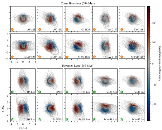
This plot shows the magnetic field structure in the stellar coronae for the final, relaxed wind solutions. The top two rows show the unscaled B_ZDI (upper) and scaled 5B_ZDI (upper middle) series wind models for the Coma Berenices wind models. The bottom two rows show the unscaled (lower middle) and scaled (lower) models for the Hercules-Lyra models. A selection of magnetic field lines are shown; the open magnetic field lines are truncated at 4R_★ to avoid crowding out the region of closed magnetic field. The stellar surface and the magnetic field lines are coloured by the local value of the radial magnetic field. The colour scale is linear from −10 to 10 G and logarithmic outside of this range. In each plot the stellar axis of rotation coincides with the plot |$\boldsymbol{\hat{z}}$| axis, and the rotational phase shown is chosen in order to permit the easy discrimination of the regions of open and closed magnetic field lines. The structure of the coronal magnetic fields appears dipole-like in spite of the excursions from a dipolar structure of the surface radial magnetic field.

From Fig. 2, it is clear that the coronal field tends towards a dipole-like structure in spite of the differences in surface magnetic field geometry, and large excursions from a dipolar structure by the radial surface magnetic field B_r that may be seen in Figs 1 and 2. This tendency indicates that the dipolar magnetogram coefficients α₁₀ and α₁₁, for which the degree ℓ = 1 in equation (1), largely govern the shape of the coronal field as one moves away from the stellar surface. This is in agreement with the complementary method of potential extrapolations of the surface magnetic field into the corona (Altschuler & Newkirk 1969; Schatten, Wilcox & Ness 1969; Hoeksema 1984; Wang & Sheeley 1992), where higher degree terms decay more rapidly with increasing |$|\boldsymbol{r}|$|⁠.

At the same time, it should be kept in mind that, in contrast to the tidy dipolar coronal fields of Fig. 2, the Sun’s magnetic large-scale field does not always resemble a dipole, especially around periods of high activity. This hints to the importance of the missing medium- and small-scale magnetic field in state-of-the-art stellar magnetograms in reconstructing the stellar coronal structure.

To emphasize the dipole-like nature of the coronal field in our wind models the rotational phase of each stellar model is chosen so that the plotted projected angle between the magnetic dipole axis and |$\boldsymbol{\hat{z}}$| is maximized and the dipole appears side-on in each panel of the figure, accentuating the structure of open and closed magnetic field lines. As in Vidotto et al. (2009) and Paper I, we see that shape of the closed field region terminates in so-called helmet streamers named after spiked military helmets (see e.g. Knötel & Sieg 1980).

While we note a general agreement between the coronal field found via potential field extrapolation methods and the relaxed fields found in our MHD models, the steady-state surface magnetic field of the MHD solution differs from the input ZDI field as given in F16 and F18 as the ZDI field includes magnetic field originating from photospheric currents. In our models, the non-radial surface magnetic field |$\boldsymbol{B}_\perp = B_\theta \boldsymbol{\hat{\theta }} + B_\varphi \boldsymbol{\hat{\varphi }}$| is found from the final, relaxed state of the MHD solution; the absence of photospheric currents in our model means that the resulting fields have only small non-potential components at the stellar surface. Jardine et al. (2013) observed in their models that the non-potential field has little influence on the large-scale magnetic geometry in the corona, and as such it is also not expected to influence the steady state stellar wind. The non-potential field does, however, represent a source of available energy to power transient expulsions of plasma and magnetic energy.

In Table 2, we give some aggregate quantities of the surface magnetic field. The |B_r| column represents the average radial field strength at the stellar surface:

$$\begin{equation*} |B_r| = \frac{1}{4\pi R_{\bigstar }^2}\oint \nolimits _{S_{\bigstar }} \left|\boldsymbol{B} \cdot \boldsymbol{\hat{n}}\right|\, \mathrm{d}S= \frac{1}{4\pi R_{\bigstar }^2}\oint \nolimits _{S_{\bigstar }} \left|B_r(\theta , \varphi)\right|\, \mathrm{d}S, \end{equation*} $$

(3)

where S_★ is the stellar surface and |$\boldsymbol{\hat{n}} \parallel \boldsymbol{\hat{r}}$| is the normal vector of S_★. The max |B_r| column gives the maximum value of the radial field strength over the stellar surface:

$$\begin{equation*} \max |B_r| = \max _{S_{\bigstar }} \left|\boldsymbol{B}\cdot \boldsymbol{\hat{n}}\right| = \max _{\theta , \varphi } \left|B_r(\theta , \varphi)\right| . \end{equation*} $$

(4)

As the radial surface magnetic field strength is a fixed boundary condition of our model, the values of |B_r| and max |B_r| do not change as the wind model is relaxed towards a steady state. The |$|\boldsymbol{B}|$| column gives the average surface field strength; the value is calculated as

$$\begin{equation*} |\boldsymbol{B}| = \frac{1}{4\pi R_{\bigstar }^2}\oint \nolimits _{S_{\bigstar }} \left|\boldsymbol{B}(\theta , \varphi)\right| \, \mathrm{d}S; \end{equation*} $$

(5)

the value of |$|\boldsymbol{B}|$| can vary during the relaxation process as |$\boldsymbol{B} = B_r\boldsymbol{\hat{r}} + \boldsymbol{B}_\perp$|⁠, of which the latter term is not a fixed boundary condition of the model. As expected, we observe that the relaxed value of |$\boldsymbol{B}$| is similar to the ‘poloidal’ magnetic field strength in F16, F18, which is unaffected by photospheric currents. The ‘Dip’, ‘Quad’, ‘Oct’ ‘16+’ columns give the percentage of magnetic energy in dipolar, quadrupolar, octupolar, and hexadecapolar and higher models in the relaxed surface magnetic field. The ℓ_.90 and ℓ_.99 columns give the degree for which 90 per cent and 99 per cent of the magnetic energy is contained in degrees equal to or lower than the tabulated value.

For each stellar model we also compute numerically the total absolute magnetic flux at the stellar surface, as well as measures of the so-called open and axisymmetric magnetic fluxes. The absolute magnetic flux across a closed surface S is given by

$$\begin{equation*} \Phi (S) = \oint \nolimits _S |\boldsymbol{B} \cdot \boldsymbol{\hat{n}}| \, \mathrm{d}S. \end{equation*} $$

(6)

where |$\boldsymbol{\hat{n}}$| is the normal vector of S. We calculate the unsigned magnetic flux at the stellar surface, which we denote Φ, and for which we also have the analytical result Φ = 4πR²|B_r|. The values of Φ are provided in Table 3. As Φ is calculated from the fixed radial magnetic field only, it does not change with time in our solution.

The total absolute magnetic flux at the stellar surface may be thought of as comprising a closed flux Φ_closed of ‘closed’ magnetic field lines that have two foot-points on the stellar surface, and an ‘open’ flux Φ_open of magnetic field lines that have only one such foot-point. In contrast to a magnetic multipole in vacuum, these open field lines extend into space, dragged by the escaping stellar wind. Closed magnetic field lines are plentiful near the stellar surface, while Φ_open ≫ Φ_closed at large distances from the star. We calculate Φ_open for each model by numerically integrating Φ(S) for a spherical surface S with a radius of many Solar radii. The resulting measure of the open flux is not sensitive to the exact radius used. The resulting values of Φ_open are given in Table 3.

The axisymmetric open flux has been linked to the cosmic ray intensity at the Earth’s surface (Wang, Sheeley & Rouillard 2006) through the formation of regions of higher magnetic field strength. The axisymmetric open flux is the integral over a spherical surface of the azimuth-averaged value of |$\boldsymbol{B}$| (Vidotto et al. 2014a):

$$\begin{equation*} \Phi _\text{axi} = \oint \nolimits _S |\boldsymbol{B}_\text{axi} \cdot \boldsymbol{\hat{n}}| \, \mathrm{d}S, \text{ where } \boldsymbol{B}_\text{axi} = \frac{1}{2\pi }\oint \boldsymbol{B} \, \mathrm{d}\varphi . \end{equation*} $$

(7)

The numerical value of Φ_axi is found by integrating equation (7) over the same surface S as is used when finding Φ_open. A quantity related to Φ_open is the open surface fraction S_open/S, the fraction of the stellar surface crossed by open magnetic field lines. We find this quantity by tracing the magnetic field lines from large number of evenly sampled points on the stellar surface.

The values of S_open in Table 3 confirms our impression that the region of closed field lines is greater for the 5B_ZDI series of models both for the Coma Berenices cluster and the Hercules-Lyra association. The region of open magnetic field lines appears about ∼35 per cent smaller for the models in the 5B_ZDI series than for the models in the B_ZDI series. This affects the wind density and speed as the regions of fast stellar wind (open field lines) are reduced; we investigate the effect of surface magnetic field strength on wind mass-loss, etc. in Section 5.1.

4.2 Alfvén surface and current sheet

When the wind speed exceeds the Alfvén speed |$u_\rm {\small A}= B / \sqrt{\mu _0 \rho }$| information cannot propagate against the flow direction. The Alfvén surface |$S_\rm {\small A}$| comprises the points where the local wind velocity |$u = u_\rm {\small A}$|⁠. As the wind accelerates with increasing distance from the star in a non-uniform way determined by the surface magnetic field, the exact shape of the Alfvén surface is determined by the magnetogram and the parameters of the coronal heating model (as described in Section 3.2). Fig. 3 shows the resulting Alfvén surface for each of the coronal fields in Fig. 2. The orientation of the plots are the same as in Fig. 2. The current sheet (Schatten 1971) where B_r = 0 is shown as a grey surface in Fig. 3. The inclination of the inner current sheet with respect to the stellar axis of rotation |$i_{B_r=0}$| (reported in Table 3) is found by fitting a plane to the inner current sheet and computing the angle between the fitted plane normal vector and the |$\boldsymbol{\hat{\Omega }}$| axis.

Figure 3.

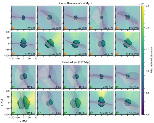
Alfvén surface and current sheet for the Coma Berenices stars (top) and the Hercules-Lyra stars bottom. The order of the panels, which is the same as in Fig. 2 is indicated by the bottom left symbols in each panel. In each group the unscaled B_ZDI models are shown in the top row and the scaled 5B_ZDI are shown in the bottom row. The z axis is parallel to the stellar axis of rotation |$\boldsymbol{\hat{z}} \parallel \boldsymbol{\Omega }$|⁠. The current sheet, for which B_r = 0 is shown as a translucent grey surface, truncated at 100R_★. The plane of sky (xz plane) and the Alfvén surface are coloured according to the local wind radial velocity. In general, we observe that the amplified magnetic fields of the 5B_ZDI models produce more irregular Alfvén surfaces.

From the plots of the Alfvén surfaces and inner current sheets in Fig. 3 we observe two-lobed Alfvén surfaces with a variety of inclinations with respect to the stellar axis of rotation. We do not observe any qualitative differences between the models of the Coma Berenices stars and the models of the Hercules-Lyra stars. Quantitative differences are considered in Section 5. As was the case in Paper I we do observe clear qualitative differences between the unscaled models and the scaled models in both Coma Berenices and Hercules-Lyra; the scaled surface magnetic field gives rise to larger Alfvén surface lobes and consequently greater values of |$R_\rm {\small A}$| and |$|\boldsymbol{r}_\rm {\small A}\times \boldsymbol{\hat{\Omega }}|$|⁠. In addition to being larger, the Alfvén surface lobes of the scaled models also tend to be more irregular, and give rise to greater wind velocities.

The large range of ‘magnetic inclinations’ in both the B_ZDI and 5B_ZDI is evident both in Fig. 3 and in the |$i_{B_r=0}$| values of Table 3. The stars AV 523 and V439 And have current sheets that are nearly aligned to the axis of rotation |$\boldsymbol{\hat{\Omega }}$|⁠, with |$i_{B_r=0}\sim {4}{^{\circ }}$| and |$i_{B_r=0}\sim {10}{^{\circ }}$| respectively, while AV 2177, DX Leo, EP Eri and HH Leo have |$i_{B_r=0}\gtrsim {75}{^{\circ }}$|⁠. The variation in |$i_{B_r=0}$| gives rise to a corresponding range of inclination of Alfvén surface lobes as can be seen in Fig. 3.

Looking at individual wind models, we observe that the two scaled models AV 523 and V439 And exhibit large Alfvén surface radii near the rotational north pole (+z direction) giving the northern Alfvén lobes of these two stars a noticeable ovoid shape also seen in Cohen & Drake (2014); the top of the ovoid is associated with rapid wind velocities. We do not see these egg-like Alfvén lobes in the unscaled AV 523 and V439 And models. We also observe some differences for the highly inclined current sheet stars between the scaled and the unscaled series of models. The Alfvén lobes of the unscaled models appear more rounded compared to the scaled models, which appear flattened near the current sheet. This flattening is sometimes accompanied by radial extrusions near the current sheet which gives the Alfvén lobe a ‘duck-billed’ appearance; this is particularly prominent in the northern Alfvén lobe of AV 1693. Similar, but thicker extrusions appear in TYC 1987, DX Leo, and HH Leo. The rapid decrease of the local Alfvén radius near the current sheet, and consequent flattening of the Alfvén surface lobe is also seen in e.g. Alvarado-Gómez et al. (2016b); these are however not as pronounced as the AV 1693 case.

The average Alfvén radius |$R_\rm {\small A}$| is the average radial distance from the stellar surface to the Alfvén surface. Considering the scalar-valued function |$\left|\boldsymbol{r}_\rm {\small A}(\theta , \varphi)\right|$|⁠, the (radial) distance at which u first exceeds |$u_\rm {\small A}$| for each point on the stellar surface S, here parametrized by the polar angle θ and the azimuth angle φ, we get

$$\begin{equation*} R_\rm {\small A}= \frac{1}{4\pi R^2}\oint \nolimits _S \left|\boldsymbol{r}_\rm {\small A}(\theta , \varphi) \right| \, \mathrm{d}S . \end{equation*} $$

(8)

The torque-averaged Alfvén distance is similarly the average value of |$\left|\boldsymbol{r}_\rm {\small A}(\theta , \varphi)\times \boldsymbol{\hat{\Omega }}\right|$| over the stellar surface:

$$\begin{equation*} \left|\boldsymbol{r}_\rm {\small A}\times \boldsymbol{\hat{\Omega }}\right| = \frac{1}{4\pi R^2}\oint \nolimits _S \left|\boldsymbol{r}_\rm {\small A}(\theta , \varphi) \times \boldsymbol{\hat{\Omega }}\right| \, \mathrm{d} S \end{equation*} $$

(9)

The |$R_\rm {\small A}$| value is a key parameter in one-dimensional models of stellar angular momentum loss (Weber & Davis 1967; Mestel 1968, 1984; Kawaler 1988). We find good agreement between the |$R_\rm {\small A}$| of this work and the dipole scaling relations of Finley & Matt (2018) based on polytropic models.

4.3 Mass-loss and angular momentum loss

The total wind mass-loss |$\dot{M}$| and total wind angular momentum loss |$\dot{J}$| are two of the most studied quantities that may be derived from stellar and Solar wind maps. Mass-loss values are difficult to constrain observationally, see the reviews of Wood (2004) and (Vidotto 2018, 2021).

From a flux argument it is clear that the mass-loss is given by

$$\begin{equation*} \dot{M} = \oint \nolimits _S \rho \boldsymbol{u} \cdot \boldsymbol{\hat{n}} \, \mathrm{d} S, \end{equation*} $$

(10)

where S is a closed surface surrounding the star and |$\boldsymbol{u}$| is the local wind velocity.

The total wind angular momentum loss can be extrapolated from observed trends between stellar periods of rotation and stellar ages (Skumanich 1972; Barnes 2003). For a population of stars, average values of |$\dot{J}$| on timescales of millions of years and longer may be inferred. There does not, however, appear to be any way of observing |$\dot{J}$| for a particular star at a particular time, such as the |$\dot{J}$| values of the stars in this study. An argument based on angular momentum flux (Mestel 1999; Vidotto et al. 2014a, see also Paper I) gives the steady state |$\dot{J}$| values associated with our wind models,

$$\begin{equation*} \dot{J} = \oint \nolimits _{S_\rm {\small A}} \left(\boldsymbol{\hat{z}} \times \boldsymbol{r} \cdot \boldsymbol{\hat{n}}\right) \left(P+ \frac{B^2}{2 \mu _0 } \right) + ({\rho \boldsymbol{V} \cdot \boldsymbol{\hat{n}}}) \varpi ^2 \Omega \, {\rm d} S_\rm {\small A} \end{equation*} $$

(11)

where |$\boldsymbol{\Omega }$| is the star’s angular velocity, |$\varpi = \boldsymbol{r} - (\boldsymbol{r} \cdot \boldsymbol{\hat{z}}) \boldsymbol{\hat{z}}$|⁠, |$\boldsymbol{V} = \boldsymbol{u} - \boldsymbol{\Omega }\times \boldsymbol{r}$|⁠, and |$S_\rm {\small A}$| is the Alfvén surface. In our models we observe that the ‘effective corotation’ term |$({\rho \boldsymbol{V} \cdot \boldsymbol{\hat{n}}}) \varpi ^2 \Omega$| dominates this expression at the Alfvén surface where we evaluate the integral. We note that |$\dot{J}$| may be evaluated over any closed surface enclosing the star, but this may involve the inclusion of additional terms in the integral, see Vidotto et al. (2014a). The presence of the angular velocity Ω in the (dominant) effective corotation term of equation (11) suggests that the parameter |$\dot{J} / \Omega$| may have a more direct link to the magnetic field strength and geometry; we return to this in Section 5, where we find that this is indeed the case.

4.4 Wind pressure out to 1 au

Once the stellar winds become superalfvénic, discontinuities and shocks may form in the solution. As the stellar winds in our models travel outwards everywhere and |$u_r \gg |\boldsymbol{u}_\perp |$|⁠, this typically occurs when a region of fast wind encounters a region of slower wind, giving rise to variations in the stellar wind properties such as the total wind pressure, which is shown in Fig. 4. Note that discontinuities and shock may appear whenever relative velocities exceed |$u_\rm {\small A}$| in the solution, such as for the CMEs modelled by Alvarado-Gómez et al. (2020).

Figure 4.

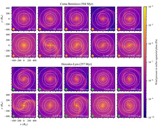
Wind pressure in the stellar equatorial plane. The order of the panels, which is the same as in Fig. 2, is indicated by the bottom left symbols in each panel. Co-rotating interacting regions (CIRs) produce multi-armed spiral structures; the number of arms depend on the geometry of the magnetic field near the stellar equator, and the amount of winding depends on the magnetic field strength and the stellar rate of rotation. Stars whose current sheet inclination is small give rise to less pronounced spiral structures. The average distances of Venus-, Earth-, and Mars-like planets are indicated by white dotted circles. When visible at this scale, the intersection of the Alfvén surface and the stellar equatorial plane is indicated by a thin black closed curve.

For a body moving through the stellar wind, such as an orbiting planet, the total wind pressure is the sum of the thermal pressure, magnetic pressure, and ram pressure,

$$\begin{equation*} P_\rm {\small W}= P+ |\boldsymbol{B}|^2 / (2 \mu _0) + \rho |\boldsymbol{u}+\boldsymbol{v}|^2 \end{equation*} $$

(12)

(see e.g. Vidotto, Jardine & Helling 2011), here |$\boldsymbol{v}$| is the planet’s orbital velocity. The quantity |$P_\rm {\small W}$| is shown in Fig. 4 with |$\boldsymbol{v}=0$| i.e. neglecting the planet’s orbital velocity. The planet’s velocity may contribute significantly to |$P_\rm {\small W}$| for close-in exoplanets but for the would-be orbits of Venus, Earth and Mars (indicated by dotted white circles in Fig. 4) we have |$|\boldsymbol{u}| \gg |\boldsymbol{v}|$|⁠. The Alfvén surface intersection with the xy-plane, outside of which the wind is superalfvénic, is shown as a thin black closed curve. Past a few stellar radii we observe that the wind pressure is dominated by the |$\rho |\boldsymbol{u}|^2$| term and that |$|\boldsymbol{u}|\approx u_r$|⁠.

In Fig. 4, we mainly observe two- and three-armed structures of locally overdense wind, while the magnetic geometry of AV 523 produces a five-armed structure. These structures arise when fast stellar wind encounters more slowly flowing wind originating from a different region of the stellar surface and are called co-rotating interacting regions (CIRs; Belcher & Davis 1971; Gosling 1996).

We also calculate the average wind pressure for an Earth-like planet using equation (12) and the Earth’s orbital elements (see Table 3). The provided value is found by averaging |$P_\rm {\small W}$| over the stellar rotational phase and the orbital phase of the Earth-like planet. As this parameter is evaluated near the stellar equator it is sensitive to variations in the current sheet inclination.

A physical body such as a planet will give rise to a shock in the wind solution if the local wind is superalfvénic. For a magnetized planet the shock forms when the magnetic pressure generated by the planet is matched by the wind pressure. The so-called magnetospheric stand-off distance is then

$$\begin{equation*} \left.R_\text{m} \middle / R_\text{p}\right. = \left(B_0^2 \middle / \left(2 \mu _0 \, \rho u^2\right)\right)^{1/6}. \end{equation*} $$

(13)

where R_p is the planet’s radius and B₀ is its dipolar magnetic field strength. For a planet with the current-day magnetic field of the Earth, we use a dipolar magnetic field of 0.7 G; which includes factor of 2 of Mead (1964) accounting for currents in the magnetosphere. The resulting distances are given in Table 3.

5 DISCUSSION

In this section, we examine trends in our results. Section 5.1 considers the effect of magnetic scaling on the model results, and Section 5.2 considers correlations within a statistical framework.

5.1 Effect of magnetic scaling

In this section, we study the effect of magnetic scaling on the models in Table 3 as well as the wind models of the Hyades stars Mel25-5, Mel25-21, Mel25-43, Mel25-151, and Mel25-179 and their scaled 5B_ZDI counterparts from Paper I. The methodology is similar to the methodology of Paper I in that the two models we have for each star allows a direct investigation of the effect of the average magnetic field strength |B|, and the residual variation caused by other factors such as magnetic geometry differences.

By having two models for each star, that vary only in their absolute radial magnetic field strength, we are able to investigate the effect of the scaling of the magnetic field on the model results. As such these results are complementary to the relations found between stellar age and wind parameters such as Vidotto et al. (2015) and Pognan et al. (2018), and the trends with age and rotation of Vidotto et al. (2014b) and Vidotto (2021). The methodology of this section disentangles the link between age and rotation rate [although the stars are too young to adhere to the Skumanich law they are still spinning down; see Gallet & Bouvier (2013) and Garraffo et al. (2018)]. The observed bimodality of the age-spin relationship (Barnes 2003) for younger stars suggests that the younger stars in the sample may be in different regimes of magnetic braking depending on their periods of rotation; we do not, however, see any clear evidence of this in our models. A possibility is that our models lie below the critical angular velocity value for fast rotators, for which values from 3 Ω_⊙ to 15 Ω_⊙ have been adopted (Kawaler 1988; Chaboyer et al. 1995; Reiners & Mohanty 2012; Amard et al. 2016). Fig. 5 shows the open magnetic flux Φ_open, the wind mass-loss rate |$\dot{M}$|⁠, the angular momentum loss rate |$\dot{J}$|⁠, the angular momentum loss rate scaled by the stellar rate of rotation |$\dot{J} / \Omega$|⁠, and the wind pressure for an Earth-like planet |$P_\rm {\small W}^{\oplus }$| plotted against the stellar unsigned surface magnetic flux Φ = 4πR²|B_r|. The values used in the plots are given in Table 3. The variation in wind pressure with stellar rotation and orbital position (true anomaly) of the Earth-like planet is indicated by boxplots.

Figure 5.

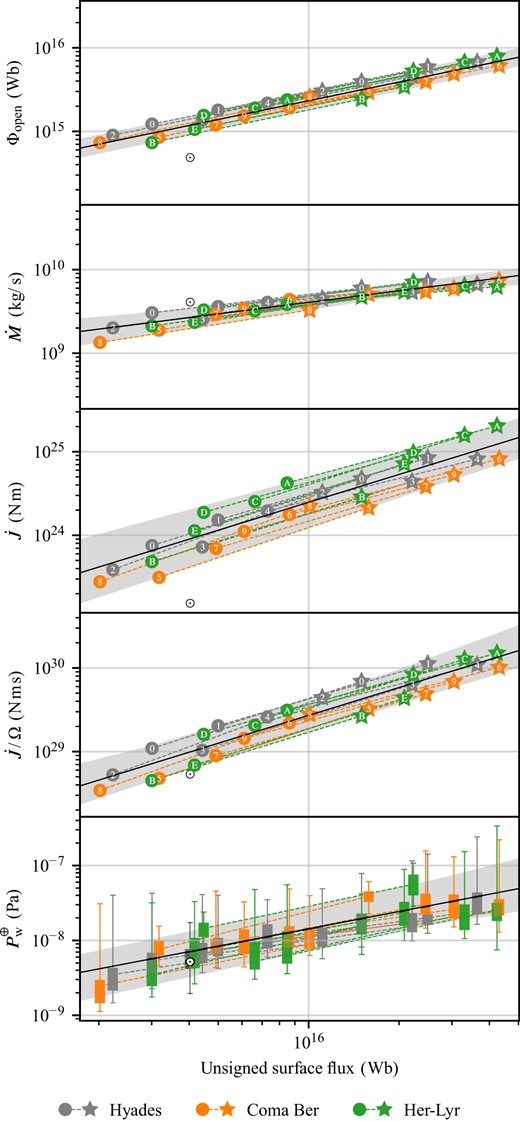
The effect of the magnetic scaling between the B_ZDI and the 5B_ZDI series and a lower bound on the residual variation. The open magnetic flux Φ_open, wind mass-loss rate |$\dot{M}$|⁠, angular momentum loss rate |$\dot{J}$|⁠, rotation-scaled angular momentum loss rate |$\dot{J} / \Omega$|⁠, and wind pressure |$P_\rm {\small W}^{\oplus }$| for an Earth-like planet is shown against the unsigned surface flux Φ = 4πR²|B_r|. The variation in the wind pressure with stellar phase and planetary orbital phase is shown as boxplots. The shaded region represents the total variation in the dashed fitted barbell power-law lines, and the solid black power-law line represents their midpoint. The y scale is the same in each panel, permitting a visual comparison of the slopes of the mid-point lines and the width of the residual variation between panels. The grey symbols and the Sun symbol represents the Hyades models and the Solar maximum wind model Sun-G2157 from Paper I. A more statistically rigorous approach to analysing the residual variation is given in Section 5.2 and Fig. 6.

We have also found that the unsigned surface flux better predicts the model output values than the average surface radial field strength B_r, hence we use the unsigned surface flux Φ as the independent variable in our fits.

For each star modelled, Fig. 5 shows a barbell comprising a circle representing the star’s B_ZDI series value, a star symbol representing the star’s 5B_ZDI series value (i.e. the symbols of Table 3), and a dashed line segment connecting the two. Each line segment has an equation of the form

$$\begin{equation*} \log _{10} \hat{y}_i(x) = \alpha _i \log _{10} x + \log _{10}\beta _i, \text{ so that } \hat{y}_i(x) \propto x^{\alpha _i} \end{equation*} $$

(14a)

i.e. a straight line in a log-log plot and a power law in linear coordinates. The index i ranges over the stars in Table 1 and the barbell connects the model output for star i in the B_ZDI with the model result for star i in the scaled 5B_ZDI series. By comparing the unscaled B_ZDI and the scaled 5B_ZDI model for each star we can see the direct influence of the magnetic field strength on the model results. The geometric midpoint and range of the slope values α_i are given in Table 4, and indicated as a black power-law line |$\hat{y}(x) = \beta x^\alpha$| in Fig. 5. To indicate the amount of variation across each of the |$\hat{y}_i(x)$| curves, the area between the |$\min _i \hat{y}_i(x)$| and |$\max _i \hat{y}_i(x)$| curves is shaded in Fig. 5.

Table 4.

Clear trends from magnetic scaling and a lower bound on residual variation. Power laws on the form |$\hat{y} \propto \Phi ^\alpha$| are able to explain a large amount of the variation in the quantities of Tables 2 and 3. The α coefficients and their associated uncertainty indicate the mid-point of the power laws on the form |$\hat{y}_i(x) \propto \Phi ^{\alpha _i}$| and the range of α_i coefficients are indicated by the range on α. A measure of the residual variation that cannot be attributed to variations in Φ is given by the |$\frac{y_\text{max}}{y_\text{min}}$| values. Aside from |$\dot{J}$|⁠, the largest residual variation is found for |$P_\rm {\small W}^{\oplus }$| and |$\dot{J} / \Omega$|⁠, suggesting that the magnetic geometry plays a large role in the determination of these quantities. The coefficients of determination (the r² values) also show the residual variation after the fit to Φ independently of the value of the exponent α, hence the two last rows have the same r² value.

Quantity	Correlation with log10Φ
	|$\displaystyle \alpha$|	|$\frac{y_\text{max}}{y_\text{min}}$|	r2
log10|Br|	1.000 ± 0.000	162.2 per cent	0.976
log10max |Br|	1.000 ± 0.000	186.4 per cent	0.937
|$\log _{10}|\boldsymbol{B}|$|	0.983 ± 0.011	165.3 per cent	0.973
|$\log _{10} R_\rm {\small A}$|	0.394 ± 0.031	164.2 per cent	0.907
|$\log _{10} |\boldsymbol{r_\rm {\small A}} \times \boldsymbol{\hat{\Omega }}|$|	0.394 ± 0.032	171.0 per cent	0.877
log10Φopen	0.745 ± 0.023	168.4 per cent	0.945
|$\log _{10}\dot{M}$|	0.439 ± 0.090	203.5 per cent	0.883
|$\log _{10}\dot{J}$|	1.094 ± 0.118	568.2 per cent	0.871
|$\log _{10}(\dot{J}/\Omega)$|	1.094 ± 0.118	310.7 per cent	0.913
|$\log _{10}P_\rm {\small W}^{\oplus }$|	0.736 ± 0.162	479.3 per cent	0.693
log10Rm	−0.123 ± 0.027	129.8 per cent	0.693

Table 4 also gives a geometric measure of the residual variation around the mid-point power-law line; these y_max/y_min values represent the largest range of residuals in the fitted region X_★

$$\begin{equation*} \frac{ y_\text{max}}{ y_\text{min}} = \max _{x \in X_{\bigstar }} \, { \frac{\max \hat{y}_i(x)}{\min \hat{y}_i(x)} }, \quad X_{\bigstar } = (\min {\Phi }_{\bigstar }, \, \max {\Phi }_{\bigstar }), \end{equation*} $$

(14b)

i.e. the largest ‘height’ of the shaded region in Fig. 5. We also give the coefficients of determination (r²-values) for the geometric mid-point |$\hat{y}(x)$| power-law lines as they provide a measure of the quality of the fit without being influenced by the magnitude of the fitted α coefficient. The r² values are given by

$$\begin{equation*} r^2 = 1 - \left. \sum {\big (\log _{10} y_j / \bar{y} \big)^2} \middle / \, \sum {\big (\log _{10} y_j / \hat{y}(x_j) \big)^2} \right. ; \end{equation*} $$

(14c)

this is the standard (e.g. Draper 1998) definition of r² subject to the logarithm identities |$\log y_j - \log \bar{y} = \log y_j/\bar{y}$| and |$\log y_j - \log \hat{y}(x_j) = \log y_j/\hat{y}(x_j)$|⁠, and where |$\bar{y}$| is the mean of the y-values. Note that in calculating the r² values the j index ranges over the models in both the scaled and the unscaled series (i.e. all the rows in Table 3), so that x_j and y_j represent the result of an individual model. It bears repeating (see Paper I) that the quantities α, y_max/y_min and r² are independent of any assumption about the statistical distribution of the model results. An analysis requiring some mild statistical assumptions is given in Section 5.2.

The middle panel of Fig. 5 suggests decreasing trend in |$\dot{J}$| with stellar age between the Hercules-Lyra association (aged 257 ± 46 Gyr) and the Coma Berenices cluster (aged 584 ± 10 Gyr). The presence of the dominating effective corotation term |$(\rho \boldsymbol{V} \cdot \boldsymbol{\hat{n}}) \varpi ^2 \Omega$| in equation (11) describing the total angular momentum loss suggests that by scaling the angular momentum loss by the stellar rate of rotation will produce a tighter correlation with Φ; we see that this is indeed the case in the fourth panel of Fig. 5, where |$\dot{J} / \Omega$| is plotted against Φ. The Hyades (aged 625 ± 50 Myr) wind models from Paper I lie between the Hercules-Lyra models and the Coma Berenices models when plotting |$\dot{J}$|⁠, and they are a bit higher than the average when plotting |$\dot{J}/\Omega$| against Φ. The overall spread is however reduced even when including the Hyades wind models.

We briefly note some key features seen in Table 4 and Fig. 5:

• We see that |B_r| and max |B_r| are proportional to Φ and as such have α = 1; this is enforced by the model and methodology as, for each star, the relation between Φ, |B_r| and max |B_r| are linear. The variation in these parameters are caused by the variation in the magnetogram geometry and quantified by y_max/y_min in Table 4.

• The average surface magnetic field strength |$|\boldsymbol{B}|$| is closely correlated with Φ as well, indicating that the radial magnetic field, rather than rotation effects determine the non-radial components of |$\boldsymbol{B}$|⁠.

• As in Paper I the Alfvén radius |$R_\rm {\small A}$| and the torque-averaged Alfvén radius exhibit very similar correlation coefficients α ≈ 0.39 and similar variation measures and coefficients of determination.

• With a larger number of stars (15 versus 5) in comparison to Paper I, we expect to see larger variation and higher values of the variation measure as it is a lower bound on the population variation and can only increase with increasing numbers of stellar models being included. We do observe larger variations in Φ_open, |$\dot{M}$|⁠, |$\dot{J}$|⁠, |$P_\rm {\small W}^{\oplus }$| and R_m compared to Paper I.

• The scaled angular momentum |$\dot{J}/\Omega$| exhibits a smaller variation y_max/y_min than |$\dot{J}$| itself as was seen in Fig. 5; the variation measure is 311 per cent and 568 per cent, respectively.

• The inclusion of |$\dot{J}/\Omega$| means that the wind pressure for an Earth-like planet |$P_\rm {\small W}^{\oplus }$| is the parameter that is least well predicted by Φ.

5.2 Statistical trends and correlations

In this section, we apply an ordinary least square (OLS) fit to the models of the B_ZDI and 5B_ZDI series. This approach is complementary to the approach in Section 5.1 where the effect of the magnetic scaling on each star model was investigated. The ordinary least square fit may be less geometrically intuitive than the effect of magnetic scaling, but the powerful statistical machinery of OLS does permit a more quantitative approach. By log-transforming our data they satisfy the assumptions required by OLS (see e.g. Draper 1998) including homoscedasticity and normality. As well as the trends themselves, OLS permits a quantitative analysis of the residual variation in the data set, expected to correspond to variations in magnetic geometry.

Fig. 6 shows trend lines (dashed black lines), confidence bands (dark grey regions) and prediction bands (light grey regions) for the mass-loss, angular momentum loss, scaled angular momentum loss, wind pressure at 1 au, and magnetospheric stand-off distance for an Earth-like planet plotted against the surface radial magnetic field strength, the unsigned surface flux, and the unsigned open flux. Select statistical parameters relating to Fig. 6 are given in Table 5. We provide the a parameter with a 95 per cent confidence interval, the coefficients of determination, the p-values, and a measure y_0.975/y_.025 of the mean size of the prediction interval at the data points of the B_ZDI series and the 5B_ZDI series; this value represents a measure of the height of the light grey shaded prediction band region in Fig. 6. The reported statistical parameters are calculated in the standard way (see e.g. Draper 1998) using the statsmodels Python package (version 0.12.1, Seabold & Perktold 2010). In comparison to the shaded residual variation in Fig. 5 and the y_max/y_min values in Table 4, the light grey shaded prediction bands in Fig. 6 are wider and the y_0.975/y_.025 values (Table 5) are greater. The bands in Fig. 5 are a geometric measure of the minimum variation and, as such, they are a lower bound on the variation attributed to differences in magnetic geometry. Prediction bands, such as the light grey 95 per cent prediction bands in Fig. 6, come with the different guarantee that, as long as the OLS assumptions are not violated, 95 per cent of new wind models with similar parameters to the ones in this study would fall inside the light grey shaded region.

Figure 6.

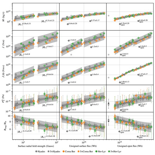
Trend lines and variation bands for (from top to bottom) mass-loss, angular momentum loss, scaled angular momentum loss, wind pressure at 1 au, and magnetospheric stand-off distance for an Earth-like planet plotted against (from left to right) the surface radial magnetic field strength, the unsigned surface flux, and the unsigned open flux. The symbols used in the plot corresponds to the tabulated values in Table 3. The dashed black lines are power-law fits made to the B_ZDI series and the 5B_ZDI series, and the dark grey regions represent confidence bands calculated at 95 per cent confidence level. The light grey regions represent prediction bands; subject to the OLS assumptions, there is a 95 per cent chance that further wind models lie inside the shaded region. Key values behind this plot are tabulated in Table 5. The Hyades wind models from Paper I (grey symbols) are included in the fits. The Solar maximum wind model Sun-G2157 from Paper I is included in the plots as a Sun symbol; this model is not included in the fits. The Solar wind parameters vary on many timescales (see e.g. Wang et al. 1998; Finley, Matt & See 2018) so the Sun-G2157 model reflects only a snapshot in time. In the two bottom rows, the point-to-point variation is indicated by boxplots.

Table 5.

Numerical summary of the fitted curves in Fig. 6. This table shows the log–log correlations between quantities of Tables 2 and 3 and the average unsigned radial field strength |B_r|, the unsigned surface magnetic flux Φ, and the unsigned open magnetic flux Φ_open. The a values columns give the exponent of the fitted power laws with 95 per cent confidence intervals. The coefficients of determination are given in the r² columns. The y_0.975/y_.025 columns give the average width of the 95 per cent prediction intervals; the average is taken over the data points of the series. The probability values (p-values) are given in the eponymous columns.

	BZDI series				5BZDI series
	a	r2	|$\frac{y_{0.975}}{y_{0.025}}$|	p	a	r2	|$\frac{y_{0.975}}{y_{0.025}}$|	p
Quantity	Correlation with alog10|Br| + b
log10max |Br|	0.94 ± 0.25	0.836	2.34	1.8 × 10−6	0.94 ± 0.25	0.836	2.34	1.8 × 10−6
|$\log _{10}|\boldsymbol{B}|$|	0.95 ± 0.03	0.997	1.12	1.5 × 10−17	0.99 ± 0.03	0.998	1.10	1.3 × 10−18
log10Φ	1.01 ± 0.20	0.900	1.99	7.4 × 10−8	1.01 ± 0.20	0.900	1.99	7.3 × 10−8
log10Φopen	0.69 ± 0.36	0.572	3.37	1.1 × 10−3	0.65 ± 0.35	0.554	3.30	1.5 × 10−3
|$\log _{10} R_\rm {\small A}$|	0.39 ± 0.15	0.705	1.67	9.1 × 10−5	0.30 ± 0.17	0.525	1.80	2.2 × 10−3
|$\log _{10} |\boldsymbol{r_\rm {\small A}} \times \boldsymbol{\hat{\Omega }}|$|	0.38 ± 0.17	0.648	1.78	2.9 × 10−4	0.30 ± 0.19	0.465	1.92	5.1 × 10−3
|$\log _{10}\dot{M}$|	0.56 ± 0.31	0.538	2.91	1.9 × 10−3	0.31 ± 0.23	0.396	2.20	1.2 × 10−2
|$\log _{10}\dot{J}$|	1.39 ± 0.76	0.546	13.26	1.6 × 10−3	1.02 ± 0.71	0.421	11.42	8.9 × 10−3
|$\log _{10}\dot{J} / \Omega$|	1.22 ± 0.67	0.543	9.74	1.7 × 10−3	0.84 ± 0.60	0.414	7.74	9.7 × 10−3
|$\log _{10}P_\rm {\small W}^{\oplus }$|	0.64 ± 0.55	0.328	6.52	2.6 × 10−2	0.59 ± 0.58	0.269	7.24	4.7 × 10−2
log10Rm	−0.11 ± 0.09	0.328	1.37	2.6 × 10−2	−0.10 ± 0.10	0.269	1.39	4.7 × 10−2
Quantity	Correlation with alog10Φ + b
log10|Br|	0.89 ± 0.18	0.900	1.91	7.4 × 10−8	0.89 ± 0.18	0.900	1.91	7.3 × 10−8
log10max |Br|	0.87 ± 0.25	0.816	2.46	4.0 × 10−6	0.87 ± 0.25	0.816	2.46	3.9 × 10−6
|$\log _{10}|\boldsymbol{B}|$|	0.84 ± 0.18	0.884	1.94	1.9 × 10−7	0.88 ± 0.18	0.891	1.95	1.3 × 10−7
log10Φopen	0.78 ± 0.21	0.825	2.18	2.9 × 10−6	0.73 ± 0.22	0.800	2.22	6.8 × 10−6
|$\log _{10} R_\rm {\small A}$|	0.38 ± 0.13	0.769	1.58	1.8 × 10−5	0.31 ± 0.15	0.616	1.70	5.3 × 10−4
|$\log _{10} |\boldsymbol{r_\rm {\small A}} \times \boldsymbol{\hat{\Omega }}|$|	0.38 ± 0.14	0.715	1.68	7.2 × 10−5	0.31 ± 0.16	0.552	1.82	1.5 × 10−3
|$\log _{10}\dot{M}$|	0.64 ± 0.20	0.788	2.06	1.0 × 10−5	0.37 ± 0.17	0.640	1.84	3.4 × 10−4
|$\log _{10}\dot{J}$|	1.55 ± 0.50	0.773	6.22	1.6 × 10−5	1.17 ± 0.53	0.637	6.88	3.6 × 10−4
|$\log _{10}\dot{J} / \Omega$|	1.39 ± 0.41	0.806	4.40	5.5 × 10−6	1.01 ± 0.42	0.679	4.54	1.6 × 10−4
|$\log _{10}P_\rm {\small W}^{\oplus }$|	0.72 ± 0.46	0.472	5.27	4.6 × 10−3	0.58 ± 0.53	0.299	6.96	3.5 × 10−2
log10Rm	−0.12 ± 0.08	0.472	1.32	4.6 × 10−3	−0.10 ± 0.09	0.299	1.38	3.5 × 10−2
Quantity	Correlation with alog10Φopen + b
log10|Br|	0.83 ± 0.43	0.572	3.80	1.1 × 10−3	0.85 ± 0.46	0.554	3.91	1.5 × 10−3
log10max |Br|	0.82 ± 0.46	0.532	4.19	2.0 × 10−3	0.85 ± 0.49	0.524	4.25	2.3 × 10−3
|$\log _{10}|\boldsymbol{B}|$|	0.78 ± 0.42	0.549	3.70	1.6 × 10−3	0.83 ± 0.46	0.538	3.97	1.9 × 10−3
log10Φ	1.06 ± 0.29	0.825	2.49	2.9 × 10−6	1.09 ± 0.33	0.800	2.65	6.8 × 10−6
|$\log _{10} R_\rm {\small A}$|	0.46 ± 0.13	0.805	1.52	5.7 × 10−6	0.43 ± 0.12	0.812	1.45	4.6 × 10−6
|$\log _{10} |\boldsymbol{r_\rm {\small A}} \times \boldsymbol{\hat{\Omega }}|$|	0.47 ± 0.14	0.791	1.56	9.3 × 10−6	0.44 ± 0.14	0.767	1.54	1.9 × 10−5
|$\log _{10}\dot{M}$|	0.78 ± 0.20	0.845	1.85	1.3 × 10−6	0.46 ± 0.20	0.667	1.80	2.0 × 10−4
|$\log _{10}\dot{J}$|	1.92 ± 0.46	0.863	4.14	5.7 × 10−7	1.61 ± 0.47	0.808	4.06	5.2 × 10−6
|$\log _{10}\dot{J} / \Omega$|	1.80 ± 0.13	0.987	1.48	1.4 × 10−13	1.47 ± 0.17	0.965	1.65	7.6 × 10−11
|$\log _{10}P_\rm {\small W}^{\oplus }$|	0.79 ± 0.57	0.408	5.81	1.0 × 10−2	0.54 ± 0.71	0.174	8.21	1.2 × 10−1
log10Rm	−0.13 ± 0.09	0.408	1.34	1.0 × 10−2	−0.09 ± 0.12	0.174	1.42	1.2 × 10−1

The dashed black trend lines on Fig. 6 are power laws on the form y(x)∝x^a; they are obtained from fitting a curve on the form

$$\begin{equation*} y(x) = b x^{a} \text{ so that } \log _{10} y(x) = \log _{10} b + a \log _{10} x \end{equation*} $$

(15)

to the set of model values. The scaling laws that are overprinted such as |B_r|^{0.56 ± 0.31} in the top left-hand panel indicate that the true value of a lies within 0.56 ± 0.31 with 95 per cent probability, so that |$\dot{M} \propto |B_r|^{0.56\pm 0.31}$| for the data in the B_ZDI series of models.

In Fig. 6, the true power law is 95 per cent likely to lie within the dark grey confidence band region surrounding the line of best fit, i.e. confidence bounds on the entire fitted curve on the form y(x) = bx^a. Furthermore, new observations are 95 per cent likely to lie within the wider light grey prediction band region. As such the height of the confidence bands represents a confidence interval on the residual variation caused by differences in the magnetic geometry and variations in the fundamental parameters of Table 1. The variance of this prediction is the sum of the variance of the fitted curve y(x) = bx^a and the mean square error of the regression, hence the light grey prediction bands are always wider than the dark grey confidence bands.

As in Fig. 5, we have included the wind models of the five Hyades stars from Paper I as well as the models of the ten stars of this work. In comparison to the similar plot in Paper I, the inclusion of all fifteen wind models in the B_ZDI and the 5B_ZDI significantly reduces the width of the 95 per cent dark grey confidence bands around the fitted curves y(x) in Fig. 6. Considering the correlations with |B_r| (the leftmost column of panels in Fig. 6), we see significant correlations for |$\dot{M}$|⁠, |$\dot{J}$|⁠, |$\dot{J}/\Omega$| in both the B_ZDI model series and the 5B_ZDI model series.

With the exception of |$P_\rm {\small W}^{\oplus }$| and R_m we find p ≤ 0.01 for all the correlations under consideration. For |$P_\rm {\small W}^{\oplus }$| and R_m we observe p ≤ 0.05 except for |$P_\rm {\small W}^{\oplus } (\Phi _\text{open})$| and R_m(Φ_open) in the 5B_ZDI series (bottom right of Table 5). The comparatively large amount of unexplained variation in |$P_\rm {\small W}^{\oplus }$| and R_m indicate that other parameters than |B_r|, Φ, and Φ_open play a large role in determining |$P_\rm {\small W}^{\oplus }$| and R_m.

In Fig. 6, we have also included the Solar maximum value from Paper I (indicated by a Sun symbol) in each panel as it falls inside the range of |B_r| values modelled in this work. The Sun model is excluded from regression analysis; it is included here for ease of comparison with the plots of Paper I.

The middle column in Fig. 6 shows correlations with the surface flux Φ (recall that Φ = 4πR²|B_r|). The most notable difference between the correlations with |B_r| (leftmost column) is that the light grey prediction bands are tighter in the correlations with Φ i.e. there is a smaller amount of unaccounted for variation when using the unsigned surface flux as the independent variable of the fit.

We also include the correlations with the open flux Φ_open in the rightmost column of Fig. 6. The light grey prediction bands are the narrowest for Φ_open, strikingly so for |$\dot{J}/\Omega$|⁠. This result indicates a very tight correlation between |$\dot{J}/\Omega$| and Φ_open produced by the awsom model. Tight correlations between Φ_open and |$\dot{J}$| and |$\dot{M}$| are the basis for parametric methods of estimating these parameters, see Réville et al. (2015). It bears repeating here that Φ_open is itself a model output so that this rightmost column of Fig. 6 is a comparison between two model outputs that cannot be known without first running the models to completion. The complementary approach of a potential extrapolation (Schatten et al. 1969; Altschuler & Newkirk 1969; Hoeksema 1984; Wang & Sheeley 1992) of the coronal magnetic field can, however, be used to estimate Φ_open, subject to the parameters of this method.

The parameter |$\dot{J}/\Omega$|⁠, which was introduced to reduce the residual variation due to differences in stellar period of rotation, exhibits reduced residual variation compared to |$\dot{J}$| for all the independent variables used in Fig. 6: |B_r|, Φ, and Φ_open. The a values found for |$\dot{J}/\Omega$| are smaller than the ones found for |$\dot{J}$|⁠, but they lie inside each other’s 95 per cent confidence intervals. The light grey prediction bands are wider for |$\dot{J}$| than for |$\dot{J}/\Omega$|⁠; numerically the width of the prediction bands may be compared by checking the y_0.975/y_.025 column in Table 5.

Comparing the slopes of curves fitted to the B_ZDI and the 5B_ZDI series in each panel, we observe that the fitted exponents to the two series are mostly compatible in the sense that the mean a value for the B_ZDI series lies inside the 95 per cent confidence interval of a for the 5B_ZDI series, and vice versa. The exceptions are the wind mass-loss parameter where there are some signs of saturation occurring at higher surface magnetic field strengths. Similar signs of saturation is seen in the awsom wind models of Alvarado-Gómez et al. (2016b) and Pognan et al. (2018) as we observed in Paper I; see also Section 5.3.

We now focus on the lower part of Fig. 6 where we plot the correlation between the wind pressure at 1 au and the resulting magnetospheric stand-off distance for an Earth-like planet R_m. While the curves of best fit have noticeable slopes for |B_r|, Φ, and Φ_open, these correlations lie around the threshold of statistical significance, indicating that |B_r| and Φ do not have strong predictive power over these values. For the Hercules-Lyra stars there appears to be a correlation between the residual and the current sheet inclination; V439 And has a low inclination while DX Leo, EP Eri, and HH Leo are highly inclined. We also see this pattern for the low inclination AV 523 and the high inclination AV 2177. These patterns appear in both the B_ZDI series and the 5B_ZDI series of models.

In Paper I, we observed a strong correlation between Φ_open and |$P_\rm {\small W}^{\oplus }$|⁠. The inclusion of the wind models from this work suggest that the tightness of this particular correlation was spurious; we now see little difference in explanatory power between the fitted curves |$P_\rm {\small W}^{\oplus } (|B_r|)$|⁠, |$P_\rm {\small W}^{\oplus } (\Phi)$|⁠, and |$P_\rm {\small W}^{\oplus } (\Phi _\text{open})$| in Fig. 6.

5.3 Comparison with known scaling laws

Many observation-based and semi-empirical scaling relations have been put forward in the literature of mass-loss and angular momentum loss against age and rotation rates.

Projecting backwards in time, Wood et al. (2002, 2005) predict mass-loss values increasing from Solar values to |${\sim }10^2 \dot{\rm M}_\odot$| at a stellar age of 0.7 Gyr, followed by lower mass-losses for even younger stars; this is the so-called wind dividing line. In our models, we do not find such a threshold but we may see some signs of saturation in |$\dot{M}$|⁠. Recently, it has been suggested that the wind dividing line might not exist as its existence is conjectured based on a few data points only; see e.g. the review of Vidotto (2021).

The modelling study of Suzuki et al. (2013) found |$\dot{M} \propto t^{-1.23}$| and no saturation of |$\dot{M}$| for very young stars; the model predicts mass-loss values of |${\sim } 2 \times 10^{2} \dot{M}_\odot$| for the Hyades and Coma Berenices, and of |${\sim } 5 \times 10^{2} \dot{M}_\odot$| at the age of the Hercules-Lyra association.

These values are significantly higher than the mass-loss values found from MHD studies similar to our own. In Paper I, we compared our stellar wind models to a large sample of literature values including the awsom based models of Alvarado-Gómez et al. (2016b), and the hot corona ideal MHD models of Llama et al. (2013), Vidotto et al. (2015), Nicholson et al. (2016), do Nascimento et al. (2016), Ó Fionnagáin et al. (2019). and the hybrid models of Pognan et al. (2018), as well as the pluto code MHD models of Réville et al. (2016). The mass-loss and angular momentum loss found in these studies are compared to our own in Fig. 7.

Figure 7.

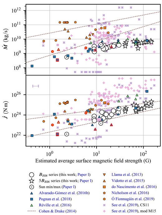
Comparison of wind mass |$\dot{M}$| and angular momentum loss |$\dot{J}$| values of this study and Paper I with literature values. The white Sun symbols, circles, and stars represent wind model results from this work and Paper I. The black and red outlined symbols represent three-dimensional MHD simulations of stars and the Sun respectively. The colour of these symbols represent the model type: blue for awsom, orange for ideal MHD, and green for the pluto model. The symbols with no outline represent populations of stars to which scaling laws have been applied; for these the interval in the upper left corner of the |$\dot{J}$| panel indicates the uncertainty in our estimates of the |B| values. When clusters of data points with identical |$\dot{M}$| values are seen they refer to the same star at different epochs. The brown dashed lines refer to the scaling laws of Cohen & Drake (2014) with Sun-like coronal densities 2 × 10¹⁴ to 2 × 10¹⁵ particles per cubic meter and a rotational period of 10 d. CS11 and mod M15 refers to different methods used by See et al. (2019). A detailed description of many aspects of this plot is available in Paper I.

We also include a comparison with the scaling laws of Cohen & Drake (2014) for two different coronal number densities of |$n = 2 \times 10^{14}{\, \mathrm{m}^{-3}}$| and |$n = 2 \times 10^{15}{\, \mathrm{m}^{-3}}$|⁠, both with a period of rotation of 10 d. Decreasing the period of rotation shifts the curve upwards. The stellar populations of See et al. (2017, 2019) are also included in Fig. 7. For the differences between the CS11 and mod M15 methodologies we refer the reader to the See et al. (2019) and the short discussion in Paper I. Due to inconsistent reporting of magnetic quantities between different studies, the quantity |B| has in some cases been estimated from other parameters; the methodology applied is described in Paper I.

From Fig. 7 it is clear that our model results show good comparison with the awsom based models of Alvarado-Gómez et al. (2016b), the hybrid models of Pognan et al. (2018) and the pluto code models of Réville et al. (2016), particularly for |$\dot{M}$|⁠. The ideal MHD models and the populations of See et al. (2017, 2019), on the other hand, predict significantly higher values of both |$\dot{M}$| and |$\dot{J}$|⁠.

We note here that some ideal MHD studies such as Ó Fionnagáin et al. (2019) also find evidence of saturation in |$\dot{J}$| as a function of rotational angular velocity Ω, but not necessarily in |$\dot{J}$| as a function of |$\boldsymbol{B}$|⁠. Compared to Paper I, we essentially see a continuation of the trends observed for the Hyades, as previously discussed in Sections 5.1–5.2.

For wind pressure and magnetospheric stand-off distance estimates, a wide range of values have been reported in the literature. Comparing to three recent studies, we find our |$P_\rm {\small W}^{\oplus }$| and R_m/R_p values occupying a middle range. Studying radio emissions of close-in exoplanets, See et al. (2015) modelled the wind ram pressure of the stars HD184733, HD179949, and τ Boötis, at orbital distances of 0.03–0.05 au and found wind ram pressures of ∼1.4 μPa ∼0.33 μPa and ∼0.23 μPa for rotation periods of 12.5, 7.6, and 3.31 d, respectively, using a potential field extrapolation of the coronal magnetic field and the Wang-Sheeley-Arge (Wang & Sheeley 1990; Arge & Pizzo 2000) method for determining wind velocity. At a similar close-in distance, our models give wind pressure values around 1 μPa for the B_ZDI series, and 10 μPa for the 5B_ZDI series; our models thus give nearly an order of magnitude higher pressure values.

In their Solar wind in time study, Ó Fionnagáin & Vidotto (2018) derived two scaling laws: one for wind ram pressure at 1 au as a function of age, and one for wind pressure as a function of rotational angular velocity. Their models incorporate a break at around 1.4Ω_⊙ or 2 Gyr, before which the magnetospheric stand-off distance R_m∝Ω^−0.32; the model predicts R_m/R_p values of 3–5 for rotational periods of 5 d to 12 d. The detailed MHD models Sun-Earth wind-planet interactions by Carolan et al. (2019) used P_ram∝Ω^0.27 for the wind ram pressure, and also found R_m values R_m/R_p values of 3–5 for rotational periods in the range 3 –13 d. Both these value ranges are smaller than our magnetospheric stand-off distance R_m/R_p range of 6–10, and predict wind pressure |$P_\rm {\small W}$| values ∼50 times greater than ours, given the |$R_\text{m}\propto P_\rm {\small W}^{-1/6}$| relation of equation (13).

Although the comparisons made here are rudimentary, it seems clear that a wide range of wind pressure values have been reported in the literature. The large range of values is a consequence of the uncertainties surrounding |$\dot{M}$| (see Fig. 7) as the ram pressure P_ram∝ρu² and the wind mass-loss |$\dot{M} \propto \rho u$| depend on the same hard-to-characterize quantities of wind density ρ and speed u. The detection of radio emissions from close-in exoplanets could potentially help constrain |$\dot{M}$| and |$P_\rm {\small W}$| in the future (see e.g. Ó Fionnagáin et al. 2019; Kavanagh et al. 2021).

6 CONCLUSIONS

We have modelled the winds of ten young, Solar-type stars in the Hercules-Lyra association and the Coma Berenices cluster aged ∼0.26 and ∼0.58 Gyr, respectively. By driving a state-of-the-art Solar system code bats-r-us/awsom, we obtain fully three-dimensional wind maps of the stars’ coronae and inner astrospheres. To account for the uncertain average magnetic field strength in ZDI (e.g. Lehmann et al. 2019), we create a second series of wind models, the 5B_ZDI series where the surface magnetic field strength is increased by a factor of 5, so that the magnetic energy is 25 times greater than in the unscaled B_ZDI models. Combining these results with our previous models of similar stars in the Hyades (aged ∼0.63 Gyr), published in Paper I, gives a large sample of 2 × 15 wind models.

The complicated surface magnetic field geometries all give rise to dipole-like coronal magnetic fields and two-lobed Alfvén surfaces. The inclination of the dipole-like coronal magnetic fields take on a range of values seemingly in the full 0^○ to 90^○ range. The 5B_ZDI series of wind models give rise to larger, more complex Alfvén surfaces, larger wind speeds, and larger regions of closed magnetic field lines.

The effect of the magnetic scaling between pairs of stellar wind models in the B_ZDI and 5B_ZDI series in Section 5.1 shows positive correlations with the surface magnetic flux for all considered parameters except, as expected, for the magnetospheric stand-off distance |$R_\text{m} \propto (P_\rm {\small W}^{\oplus })^{-1/6}$|⁠. The largest amount of residual variation is found for |$\dot{J}$| and the second largest amount of residual variation is found for |$P_\rm {\small W}^{\oplus }$|⁠. By controlling for the stellar rate of rotation in the |$\dot{J}/\Omega$| parameter the largest amount of residual variation is |$P_\rm {\small W}^{\oplus }$| where the inclination of the magnetic axis appears to play a role.

The conclusions of the geometric analysis of the effect of magnetic scaling in Section 5.1 is strengthened by the complementary statistical analysis of the B_ZDI and 5B_ZDI series as separate populations in Section 5.2. Here, we find 95 per cent confidence intervals on the predicted total range of variation of wind models of young Solar-type stars in our age range of ∼0.26 to ∼0.63 Gyr. The intervals correspond to a variation of ∼2 in |$\dot{M}$| values and ∼4.5 in |$\dot{J} / \Omega$| values. The large effect of the stellar rate of rotation is evident as the variation in |$\dot{J}$| itself is a factor of 6–7.

There appears to be growing (Garraffo et al. 2016; Dong et al. 2018; Airapetian et al. 2021; Kavanagh et al. 2021; Ó Fionnagáin et al. 2021) interest in scaling the Poynting flux-to-field ratio |$\Pi _\rm {\small A}/B$|⁠; variations in this parameter affect the steady-state wind mass-loss as |$\dot{M}$| is roughly proportional to |$\Pi _\rm {\small A}/B$| (Boro Saikia et al. 2020). Airapetian et al. (2021) scaled |$\Pi _\rm {\small A}/B$| by a factor of 27 when modelling the young Solar-type star κ¹ Ceti based on far-UV observations. In this work where we use the Solar |$\Pi _\rm {\small A}/B$| value and considered a scaled 5B_ZDI magnetic field, thus the mass-loss rates do not go as high as in ideal MHD models. If a scaling of 27 or more of the Poynting flux is realistic for young, Solar-type stars, it means that many wind parameters of this work are underestimated by an order of magnitude. This could close the gap between ideal MHD models and the awsom wind models observed in Section 5.3. More research on constraining the value of this parameter for young Solar-type stars would therefore be of interest.

We do not observe any sign of the ‘wind dividing line’ of (Wood et al. 2004, 2005) in our wind models, this is expected as the effect of photospheric currents and the resulting toroidal magnetic field is not part of the wind model input. The toroidal magnetic field is not expected to influence the steady state wind, but the toroidal magnetic energy would serve as an energy reservoir for transient events such as flares and coronal mass ejections (Jardine et al. 2013).

We do not observe any clear trends between the effective magnetogram degree estimates ℓ_.90 and ℓ_.99 in Section 4.1 and the model derived quantities in Section 5. The large variations in wind parameters found by Garraffo, Drake & Cohen (2015) for pure quadrupolar and higher degree fields do not seem to appear easily when driving the model with ZDI-derived mixed degree surface magnetic fields.

The wind models in this work are in weak agreement with the studies of Finley & Matt (2018) and See et al. (2019) which suggested that the dipolar magnetic field component dominates the wind angular momentum loss when wind mass-loss does not exceed a threshold value; the mild saturation we observe in mass-loss with increasing surface magnetic field strength does however mean that all the wind models in this work lay below the threshold value of mass-loss.

It was noted by Finley et al. (2018) that two-temperature MHD models such as bats-r-us/awsom, that recover the bimodality of the fast and slow solar wind, have not yet been used to formulate scaling relations. With the set of 2 × 15 wind models and resulting scaling laws provided here, this work may represent a small contribution to addressing this issue.

ACKNOWLEDGEMENTS

DE is funded by a University of Southern Queensland (USQ) International Stipend Research Scholarship (ISRS) and a USQ International Fees Research Scholarship (IFRS). This research was undertaken using the University of Southern Queensland (USQ) Fawkes HPC which is co-sponsored by the Queensland Cyber Infrastructure Foundation (QCIF), see www.usq.edu.au/hpc. This work has made use of the Vienna Atomic Line Database (VALD), operated at Uppsala University, the Institute of Astronomy RAS in Moscow, and the University of Vienna. We acknowledge the use of the SIMBAD database. This research has made use of the VizieR catalogue access tool, CDS, Strasbourg, France (DOI: 10.26093/cds/vizier). The original description of the VizieR service was published in A&AS 143, 23. This research has made use of NASA’s Astrophysics Data System. This work was carried out using the swmf tools developed at The University of Michigan Center for Space Environment Modelling (CSEM) and made available through the NASA Community Coordinated Modelling Center (CCMC).

This work has made use of the following additional numerical software, statistics software and visualisation software: numpy version 1.19.4 (van der Walt, Colbert & Varoquaux 2011), scipy version 1.5.3 (Virtanen et al. 2020), matplotlib version 3.3.3 (Hunter 2007), statsmodels version 0.12.1 (Seabold & Perktold 2010), tecplot version 2020.2.0.110596, and pytecplot version 1.3.3.

We would also like to thank the anonymous referee for their prompt response and diligence in helping to improve this manuscript.

DATA AVAILABILITY

The data underlying this article will be shared on reasonable request to the corresponding author.

Footnotes

1

In the context of this paper, an ‘Earth-like planet’ means that we use the orbital elements of the Earth along with the Earth’s radius and current-day dipolar magnetic field strength.

2

http://ipag.osug.fr/Anr_Toupies/

3

http://polarbase.irap.omp.eu/

4

Negative values of m would provide redundant degrees of freedom as the imaginary part equation (1) is discarded.

APPENDIX: POOLED SERIES

Here, present the same analysis as in Section 5.2, but for a pooled data series comprising the values in both the B_ZDI and the 5B_ZDI series. The fitted curves are found in Fig. A1 and the corresponding data is found in Table A1. Pooling the data gives a single series of data with a larger range of |B_r| values and 2 × 15 = 30 data points.

Figure A1.

Trend lines and variation bands as in Fig. 6, but treating the B_ZDI and 5B_ZDI series as a single population. The fitted curve is also described in Table A1.

Table A1.

This table is similar to Table 5, but for the pooled series comprising all the models of both the B_ZDI and 5B_ZDI series. As the fitted curves here maximize the coefficients of determination, the r² values are higher than the r² values of the geometric mid-point approach in Table 4.

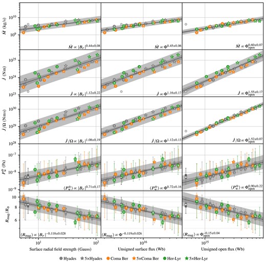
	a	r2	|$\frac{y_{0.975}}{y_{0.025}}$|	p
Quantity	Correlation with alog10|Br| + b
log10max |Br|	0.99 ± 0.07	0.964	2.14	1.0 × 10−21
|$\log _{10}|\boldsymbol{B}|$|	0.98 ± 0.01	0.999	1.11	5.0 × 10−46
log10Φ	1.00 ± 0.06	0.977	1.84	1.9 × 10−24
log10Φopen	0.73 ± 0.11	0.878	2.93	2.5 × 10−14
|$\log _{10} R_\rm {\small A}$|	0.38 ± 0.05	0.902	1.65	1.3 × 10−15
|$\log _{10} |\boldsymbol{r_\rm {\small A}} \times \boldsymbol{\hat{\Omega }}|$|	0.38 ± 0.05	0.881	1.75	1.9 × 10−14
|$\log _{10}\dot{M}$|	0.44 ± 0.08	0.802	2.37	2.3 × 10−11
|$\log _{10}\dot{J}$|	1.12 ± 0.22	0.793	9.55	4.3 × 10−11
|$\log _{10}\dot{J} / \Omega$|	1.08 ± 0.19	0.828	7.03	3.3 × 10−12
|$\log _{10}P_\rm {\small W}^{\oplus }$|	0.71 ± 0.17	0.728	5.58	2.1 × 10−9
log10Rm	−0.12 ± 0.03	0.728	1.33	2.1 × 10−9
Quantity	Correlation with alog10Φ + b
log10|Br|	0.97 ± 0.06	0.977	1.83	1.9 × 10−24
log10max |Br|	0.97 ± 0.08	0.957	2.29	1.2 × 10−20
|$\log _{10}|\boldsymbol{B}|$|	0.95 ± 0.06	0.974	1.87	1.0 × 10−23
log10Φopen	0.75 ± 0.07	0.948	2.01	1.5 × 10−19
|$\log _{10} R_\rm {\small A}$|	0.38 ± 0.04	0.921	1.57	6.2 × 10−17
|$\log _{10} |\boldsymbol{r_\rm {\small A}} \times \boldsymbol{\hat{\Omega }}|$|	0.38 ± 0.05	0.901	1.66	1.4 × 10−15
|$\log _{10}\dot{M}$|	0.45 ± 0.06	0.885	1.93	1.1 × 10−14
|$\log _{10}\dot{J}$|	1.16 ± 0.17	0.874	5.83	4.1 × 10−14
|$\log _{10}\dot{J} / \Omega$|	1.12 ± 0.13	0.913	4.01	2.3 × 10−16
|$\log _{10}P_\rm {\small W}^{\oplus }$|	0.72 ± 0.16	0.761	5.02	3.4 × 10−10
log10Rm	−0.12 ± 0.03	0.761	1.31	3.4 × 10−10
Quantity	Correlation with alog10Φopen + b
log10|Br|	1.20 ± 0.17	0.878	3.98	2.5 × 10−14
log10max |Br|	1.20 ± 0.18	0.867	4.28	9.0 × 10−14
|$\log _{10}|\boldsymbol{B}|$|	1.18 ± 0.17	0.873	4.00	4.8 × 10−14
log10Φ	1.27 ± 0.11	0.948	2.49	1.5 × 10−19
|$\log _{10} R_\rm {\small A}$|	0.51 ± 0.05	0.947	1.45	2.2 × 10−19
|$\log _{10} |\boldsymbol{r_\rm {\small A}} \times \boldsymbol{\hat{\Omega }}|$|	0.51 ± 0.05	0.938	1.50	2.0 × 10−18
|$\log _{10}\dot{M}$|	0.60 ± 0.07	0.906	1.81	6.1 × 10−16
|$\log _{10}\dot{J}$|	1.55 ± 0.17	0.927	3.82	1.9 × 10−17
|$\log _{10}\dot{J} / \Omega$|	1.52 ± 0.07	0.987	1.71	5.3 × 10−28
|$\log _{10}P_\rm {\small W}^{\oplus }$|	0.90 ± 0.22	0.707	5.96	6.0 × 10−9
log10Rm	−0.15 ± 0.04	0.707	1.35	6.0 × 10−9

In Paper I, we observed the that the correlations in the |B_r| improved and seemed to approach the correlations in the Φ_open series. The addition of the data points of this work show that this effect was largely spurious except for the wind pressure for an Earth-like planet and the magnetospheric stand-off distance. The other parameters |$\dot{M}$|⁠, |$\dot{J}$|⁠, and the new parameter |$\dot{J}/\Omega$| have a significantly tighter correlation with Φ_open than with |B_r|, with Φ occupying a middle ground.

When considering the pooled series and its large B_r range it should be kept in mind that here, the rotation-field strength correlation (Noyes et al. 1984; Vidotto 2018) is adjusted for. This is different from studies of stars over a large age range, such as Vidotto et al. (2015) and Pognan et al. (2018), where this correlation, being one of the objects of study, is intentionally present in the final results.