3DNA: a software package for the analysis, rebuilding and visualization of three‐dimensional nucleic acid structures

Abstract

We present a comprehensive software package, 3DNA, for the analysis, reconstruction and visualization of three‐dimensional nucleic acid structures. Starting from a coordinate file in Protein Data Bank (PDB) format, 3DNA can handle antiparallel and parallel double helices, single‐stranded structures, triplexes, quadruplexes and other complex tertiary folding motifs found in both DNA and RNA structures. The analysis routines identify and categorize all base interactions and classify the double helical character of appropriate base pair steps. The program makes use of a recently recommended reference frame for the description of nucleic acid base pair geometry and a rigorous matrix‐based scheme to calculate local conformational parameters and rebuild the structure from these parameters. The rebuilding routines produce rectangular block representations of nucleic acids as well as full atomic models with the sugar–phosphate backbone and publication quality ‘standardized’ base stacking diagrams. Utilities are provided to locate the base pairs and helical regions in a structure and to reorient structures for effective visualization. Regular helical models based on X‐ray diffraction measurements of various repeating sequences can also be generated within the program.

Received May 1, 2003; Revised and Accepted June 25, 2003

INTRODUCTION

The hydrogen bonding and stacking of the nitrogenous bases are fundamental to the organization of DNA and RNA, shaping both their three‐dimensional structures and modes of recognition. The canonical Watson–Crick base pairs used to encode genetic information in double helical DNA (1) represent only one of the many possible edge‐to‐edge interactions of base residues. A rich variety of alternative base pairing motifs (2) underlies the multitude of structural forms adopted by RNA, e.g. rRNA (3), and the multi‐stranded complexes of DNA, e.g. DNA tetraplexes (4,5). Furthermore, the base pairs are not necessarily planar and bifurcated (three center) hydrogen bonding may stabilize long arrays of stacked bases (6,7). The face‐to‐face stacking of aromatic rings, which persists even in the absence of base pairing (8–10), depends subtly on nucleotide sequence. For example, the degree of stacking overlap, as measured by the orientation and displacement of successive Watson–Crick base pairs, is greater at certain DNA dimer steps and smaller at others (11,12).

The ionic character of the sugar–phosphate backbone makes the nucleic acids especially sensitive to local environment, with ligand interactions frequently leading to a change of conformational state (13–16). The tendency of DNA and RNA to associate with ligands and the ease of conformational change are also dependent on sequence. For example, pyrimidine–purine dimers stand out as highly flexible steps in protein–DNA complexes (17) and GG·CC dimers as steps which are easily converted by drugs and proteins to A‐type geometries (18).

Development of a framework for understanding the three‐dimensional structures and interactions of nucleic acids calls for quantitative methods which describe the spatial arrangements of the constituent molecular fragments and also allow for the reconstruction of molecular models from derived parameters. A 1988 workshop established conceptual guidelines for specifying the orientation and displacement of complementary bases and successive base pairs in double helical structures (19), and a standard base‐centered reference frame was recently recommended for use in nucleic acid structural studies (20). A nomenclature has also been established for the description and classification of RNA base pairing (21), and various computer programs have been developed for the identification and description of RNA base pairs and structural motifs (22–27). Surprisingly, the latter studies do not take advantage of the principles and methods widely used in the analysis of DNA structure (12,28–35). Moreover, the programs used to date to characterize nucleic acid–ligand interactions (36–39) are not capable of identifying ligand‐induced conformational changes in DNA or RNA.

Here we present a comprehensive software package for the analysis, reconstruction and visualization of three‐dimensional nucleic acid structures. The program, entitled 3DNA, can be applied to parallel and antiparallel double helices, single‐stranded forms, multi‐stranded helices and complex tertiary folding motifs found in both DNA and RNA structures. Analyses can be performed on either single crystal structures, such as those compiled in the Nucleic Acid Database (NDB) (40), or ensembles of structures generated in the course of NMR structure determination or molecular simulations. The analysis routines identify and characterize all base interactions and provide an automatic classification of appropriate double helical steps. Hydrogen bonding patterns are described in terms of the spatial displacement and orientation of standard reference frames on the interacting bases and stacking overlaps are assessed directly from planar projections of the ring and exocyclic atoms in consecutive bases or base pairs. The spatial disposition and relative orientation of sequential base pair steps are also expressed in terms of standard rigid body parameters. Conventional torsional parameters and assorted virtual distances and angles are used to characterize molecular conformation, with automatic conformational classifications based on derived parameters known to distinguish different helical forms. The automatic detection and classification of conformation are useful for pinpointing conformational transitions in ligand‐bound DNA (18), especially changes in short fragments which cannot be detected with other analysis programs. The rebuilding module produces publication quality ‘standardized’ base stacking diagrams for easy visualization of the stacking of adjacent residues and generates sequence‐dependent atomic structures in Protein Data Bank (PDB) format (41), with an approximate sugar–phosphate backbone suitable as a starting point for molecular calculations. The popular Calladine–Drew block schematic representation of DNA structure (42) can be produced, either in isolation or in combination with other graphic images. A total of 55 regular DNA and RNA helical structures, based on the fiber diffraction of extended polymers (43–52), can also be constructed for arbitrary sequences. The interchangeable description of base pair structure at a local dimeric or helical level facilitates the analysis and modeling of nucleic acid conformational transitions.

CONFORMATIONAL ANALYSIS

Identification of base pairs

3DNA starts with a least squares fitting of a standard base structure with an embedded reference frame to its experimental counterpart following the approach of Babcock et al. (29). This method uniquely defines the position and orientation, i.e. the reference frame, of each base in a structure.

The base pairing information needed for the analysis routine is generated automatically with a utility program which identifies all residues in close contact. This purely geometric approach makes use of the recently established standard base reference frame (20) and can be used to identify all possible base pairs (canonical as well as non‐canonical), higher order base associations and double helical regions in a nucleic acid structure. When applied to the refined crystal structure of the large (50S) ribosomal subunit (NDB_ID: rr0033) (3), for example, the method finds 23 of the 28 classic base pairs with at least two hydrogen bonds involving different pairs of atoms in the most stable (keto and amino) forms of the five common bases (2). Other base pairs with hydrogen bonds to backbone atoms are also identified, along with base triplets, tetrads and pentads (see examples below). Once a base pair is located on the basis of geometric criteria, the hydrogen bonding patterns are checked, allowing for the identification of unexpected pairings. Each base pair is uniquely characterized by a set of six rigid body parameters (Fig. 1, upper left), which can be used in combination with the hydrogen bonding patterns in a searchable database. Publication quality best view images of the base pairs, in various styles, with hydrogen bonds and base rings optionally color coded by residue type, can be automatically generated (see below). Modified bases are mapped to standard counterparts, e.g. 5‐iodouracil (5IU) to uracil (U) and 1‐methyladenine (1MA) to adenine (A), allowing for easy analysis of unusual DNA and RNA structures (X.‐J. Lu, Y. Xin and W.K. Olson, unpublished data). This geometrically based algorithm differs from conventional hydrogen bond searches of nucleic acid interactions, which are based on the distances between pre‐selected proton donor and acceptor atoms (25,26).

Base pair parameters

Each base has two unique faces, arising from molecular asymmetry (53,54), which can be distinguished with the standard nucleic acid base reference frame. One face, which is hatched in Figure 2, corresponds to the positive z‐axis of the base plane, and the opposing face, which is unshaded, to the negative z‐axis. For Watson–Crick base pairs, such as the A–U pair in Figure 2a, the faces of the two bases are of the opposite sense, corresponding to two antiparallel strands. More generally, when the two bases (M and N) forming a pair have opposing faces, the scalar product of their z‐axes is negative. 3DNA designates such pairs, e.g. Watson–Crick A–U, A–T and G–C pairs, as M–N with the ‘–’ symbol used to emphasize the opposing directions. If the M and N bases in a pair share the same face, such as in the Hoogsteen base pair in Figure 2b, the pair is recorded as M+N, with the ‘+’ symbol used to emphasize the similar directions of the bases. This convention is simpler but in essence the same as the normal versus flipped concept of base pairing introduced by Burkard et al. (55).

To calculate the six complementary base pair parameters of an M–N pair (Shear, Stretch, Stagger, Buckle, Propeller and Opening), where the two z‐axes run in opposite directions, the reference frame of the complementary base N is rotated about the x₂‐axis by 180°, i.e. reversing the y₂‐ and z₂‐axes in Figure 2a. Under this convention, if the base pair is reckoned as an N–M pair, rather than an M–N pair, the x‐axis parameters (Shear and Buckle) reverse their signs. For an M+N pair, e.g. the Hoogsteen A+U in Figure 2b, the x₂‐, y₂‐ and z₂‐axes do not change sign; thus all six parameters for an N+M pair are of opposite sign from those for an M+N pair.

Since the six base pair parameters uniquely define the relative position and orientation of two bases, they can be used to reconstruct the base pair. Moreover, the parameters provide a simple mechanism for classification of structures (55) and database searching (X.‐J. Lu, Y. Xin and W.K. Olson, unpublished data). Among the six base pair parameters, only Shear, Stretch and Opening are critical in characterizing key hydrogen bonding features, i.e. base pair type: Shear and Stretch define the relative offset of the two base origins in the mean base pair plane and Opening is the angle between the two x‐axes with respect to the average normal to the base pair plane (see upper left panel in Fig. 1). For the Hoogsteen A+U base pair shown in Figure 2b, Shear is 0.5 Å, Stretch –3.5 Å and Opening 70°. Buckle, Propeller and Stagger, in contrast, are secondary parameters, which simply describe the imperfections, i.e. non‐planarity, of a given base pair.

The calculation of complementary base pair parameters follows the definitions of El Hassan and Calladine (32) as implemented in SCHNAaP (34). This matrix‐based algorithm, originally formulated by Zhurkin et al. (56), is rigorous and reversible in that it allows for the exact reconstruction of a three‐dimensional structure from a set of derived parameters (see below). The parameters so defined have simple geometrical meanings. For example, the distance between the centers of a complementary base pair is the net change in translational parameters, (Sx² + Sy² + Sz²)^1/2, and the angle between base planes is the net change in (out‐of‐plane) bending parameters, (κ² + π²)^1/2 (see Fig. 1 for designation of symbols).

Treatment of non‐Watson–Crick base pairing motifs

The G–U wobble pair, a fundamental interaction involved in diverse RNA contexts (57–59), is illustrative of the non‐Watson–Crick base pairing found in nucleic acid structures. Geometrically, its key feature is a –2.2 Å Shear (+2.2 Å for the U–G pair), which breaks the structural symmetry between the C1′ atoms found in a Watson–Crick base pair.

As noted previously (20), differences in Shear between neighboring base pairs lead to the discrepancies in dinucleotide Twist reported by others (57,58,60). For example, the respective twist angles of the C7G8·U12G13 and G8C9·G11U12 dimer steps, flanking either side of the G–U wobble pair in the structure of the acceptor stem of Escherichia coli tRNA^Asp (NDB_ID: ar0019) (60) (Fig. 3), are found to be 22° and 42° with Curves (28) versus 35° and 28° with FreeHelix (35). The new standard base reference frame (20), which is implemented in 3DNA, leads to twist angles in close agreement with those obtained from Curves.

While one can correct the apparent variation in Twist at dimer steps containing G–U wobble base pairs by defining a reference frame on the non‐Watson–Crick pair different from the standard Watson–Crick reference frame (61), we adhere to the standard frame in 3DNA and use the numerical values of the base pair parameters to characterize different non‐Watson–Crick base pair interactions. All base pair parameters are thus calculated with respect to a common standard. The finely dotted lines in the representation in Figure 3 of base pairs from the 0.97 Å structure of the tRNA^Asp stem (60) provide a helpful visualization of dimeric Twist. The cross‐strand stacking of G8 over G13, with the two six‐membered rings sharing a 2.15 Ų area of common overlap, is due in large part to a combination of negative Slide (–2 Å) and positive Shift (+1.7 Å), rather than to the twisting variations attributed by Trikha et al. (57) in their analysis of the G–U containing steps in the r(GGUAUUGCGGUACC)₂ self‐complementary 14mer duplex.

The base pair parameters and hydrogen bond characteristics of a representative example of each of the 28 classic base pair types with two or more hydrogen bonds between bases (2) are listed in Supplementary Material (Table S1). As noted above, all but five of the base pairs are found in the high resolution (2.4 Å) structure of the large ribsomal subunit (NDB_ID: rr0033) (3). The remaining five examples come from other, less well‐resolved ribosomal structures, rr0014 (62), rr0020 (63), rr0025 (64) and rr0052 (65), and from the 2.6 Å resolution structure of the ternary complex of Cys‐tRNA^Cys with the translation elongation factor EF‐Tu and GTP (pr0004) (66). Further details of the base pair search algorithm and the composition and geometries of all base pairing interactions observed to date in well‐resolved RNA structures will be reported elsewhere (X.‐J. Lu, Y. Xin and W.K. Olson, manuscript in preparation).

Dimer step parameters

Six rigid body parameters (three rotations and three translations) are required to describe the position and orientation of one base pair relative to another. Two sets of such parameters are commonly used in the literature (Fig. 1, upper and lower right): the set of local base pair step parameters, Shift (Dx), Slide (Dy), Rise (Dz), Tilt (τ), Roll (ρ) and Twist (ω), which describe the stacking geometry of a dinucleotide step from a local perspective; the set of helical parameters, x‐displacement (dx), y‐displacement (dy), helical rise (h), inclination (η), tip (θ) and helical twist (Ω_h), which describe the regularity of the helix, e.g. helical twist is the angle of rotation about the helical axis that brings successive base pairs into coincidence. In 3DNA, the helical axis is defined at a local level, following Bansal et al. (31), as (x₁ – x₂) × (y₁ – y₂). This axis corresponds to the single rotational axis that brings the reference frames of successive base pairs, (x₁, y₁, z₁) and (x₂, y₂, z₂), into coincidence, and its location follows Chasles’ theorem as detailed in Babcock et al. (29). The calculations of x‐displacement, y‐displacement, tip and inclination in this reference frame are based on the definitions of Lu et al. (34).

Except for a change from the mean base pair normal used in the calculation of step parameters to a local helical axis in the determination of helical parameters, the mathematics behind the two sets of rigid body variables are identical and rigorous. Thus, one set of parameters can be deduced from the other without any loss of information (34,67). For example, from the perspective of base pair step parameters, the orientation of a given base pair with respect to its immediate predecessor is defined by the matrix product,

R_z(ω/2 – ϕ) R_y(Γ) R_z(ω/2 + ϕ),1

and in the local helical frame, the same neighbors are related by the expression:

R_z(–ϕ′) R_y(–Λ) R_z(Ω_h) R_y(Λ) R_z(ϕ′).2

Here R_u is a rotation matrix about axis u, Γ is the net bending angle, i.e. Γ = (τ² + ρ²)^1/2, and ϕ is the phase angle of bending, i.e. the angle that the Roll–Tilt hinge makes with respect to the Roll axis (68). Similarly, Λ is the angle between the base pair normal and the local helical axis, i.e. Λ = (η² + θ²)^1/2, and ϕ′ is the angle that the Tip–Inclination hinge makes with respect to the Tip axis (34). A rotation of angle Λ around the Tip–Inclination hinge aligns the base pair normal with the helical axis. In the transformed base pair reference frame (the local helical frame), Tip and Inclination are components of Λ, i.e. θ = Λ cosϕ′ and η = Λ sinϕ′. Subscripts x, y and z in equation 1 refer to the ‘middle frame’ axes and those in equation 2 to the ‘middle helical frame’ axes. Rearrangement of these equations leads to the following simple expressions between local step parameters and helical variables:

θ/η = – τ/ρ,3

2 cosΩ_h = cosω (1 + cosΓ) – (1 – cosΓ).4

Some of the relationships between the two sets of rigid body parameters, which were described qualitatively by Calladine and Drew (42) in their base‐centered model of the B to A transition of DNA, are depicted quantitatively in Figure 4a–d and in Table 1. As is clear from Figure 4d, the introduction of non‐zero Roll and Slide at each dinucleotide step changes both the global inclination and x‐displacement of base pairs. In this context, it should be noted that a pure Roll maneuver also introduces a finite global displacement of base pairs, with a Roll of 12° introduced into an ideal B‐like helix leading to an x‐displacement of –1.75 Å (Fig. 4c and Table 1), rather than the null displacement proposed by Dickerson and Ng (69). The helical rise is equal to the dimer step Rise in B DNA (Fig. 4a), but is smaller in value in A DNA, where the DNA is globally compressed via Slide and Roll (Fig. 4d). The helix is extended, however, if the sign of Roll is reversed from that in A DNA, as in Figure 4e. Whereas the helical twist and rise describe the periodicity of DNA structure, the values of Twist and Rise reflect the base pair stacking geometry at a given dimer step, i.e. Rise stays close to the 3.34 Å van der Waals’ separation distance regardless of the overall extension or compression of the double helix.

CLASSIFICATION OF DOUBLE HELICAL STEPS

Classical forms: A, B and Z DNA

Experimentally determined DNA structures fall into three major conformational classes: the right‐handed A and B helical forms and the left‐handed Z helix (70). The latter structure is distinguished in 3DNA by its left‐handed helical twist and flipped (syn) guanine base compared to the two right‐handed helices (71). The A and B DNA double helices are separated on the basis of z_P, the projection of the phosphorus atom onto the z‐axis of the dimer ‘middle frame’ (18).

Intermediate helical states

Because of the irregularities in real structures, the distinctions between A and B DNA and the intermediate AB states are not easily seen by eye. Characteristic global features of the A and B forms, such as the major and minor groove structure, become apparent only in sufficiently long chain fragments (18) and can be mistaken for other conformational perturbations, e.g. changes in the phosphodiester linkage (72), which are not necessarily indicative of the B→A transition. Thus inaccurate assignments may occur if structural analyses are not performed carefully. For example, Vargason et al. (73) recently proposed an ‘extended and eccentric’ cytosine‐rich ‘E DNA’ structure of d(GGCGCBr⁵C)₂ (NDB_ID: ud0011), said to be characterized by negative Slide and an increased helical rise. Based on a reanalysis of the structure using other programs, Ng and Dickerson (74) concluded that E DNA is not very different from what they term the AB transition state structure of d(CATGGGCCCATG)₂ (NDB_ID: bd0026) (75). With the same Curves program used by Vargason et al. (73), we find that the ‘E DNA’ classification is option‐dependent: the computed parameters depend on whether one fits or does not fit a standard base to the side groups in the experimental structure (76) and whether one chooses a curved or linear helical axis. For example, under ‘normal’ Curves options (fitting a standard base to each aromatic ring system in the structure and using a curved helix) the value of Rise is 3.30 Å, rather than the ‘extended’ value of 3.56 Å reported by Vargason et al. (73).

3DNA makes use of the z_P parameter both to distinguish A from B DNA and to identify conformational intermediates along the B→A transition pathway. Intermediate AB states are identified if the z_P values fall in the gap between the characteristic ranges found for pure A DNA (z_P > 1.5 Å) and B DNA (z_P < 0.5 Å) structures. Other parameters are needed, however, to confirm conformational assignments based on z_P alone (18). As is evident from the data in Table 2, the ‘E DNA’ structure is very A‐like in terms of z_P, but has smaller Roll and more negative Slide than the step parameters typical of most A DNA structures. The ‘E DNA’ parameters are remarkably similar to those found to characterize the A‐like structure of d(GCCCGGGC)₂ (NDB_ID: adh008) previously solved by Heinemann et al. (77). The AB transition states captured in the crystal structures of two chemically modified analogs of d(GGCGCC)₂ (78) show the intermediate positioning of phosphate groups between the characteristic z_P ranges for A and B DNA and concomitant modulation of other key parameters, e.g. the Slide adopts intermediate values. Notably, in two of these duplexes (included in Table 2) all of the base pair steps assume an intermediate AB conformational state. The AB transition state reported to occur in the structure of d(CATGGGCCCATG)₂ (75) (NBD_ID: bd0026), however, is A‐like in terms of phosphorus positioning and other conformational variables.

TA DNA

A detailed structural analysis of two early examples of the TATA‐box DNA bound to the TATA‐box binding protein (TBP) (10,79) led Guzikevich‐Guerstein and Shakked (80) to propose that the 8 bp TATA‐box adopts a novel TA‐DNA conformation, different from either A or B DNA. The structures of many more such complexes have since been determined (81) and, as shown in Table 2 and Figure 5, all TATA‐box regions share similar conformational features. Whereas z_P (18) can discriminate A‐like from B‐like base pair steps, a similarly defined parameter in the helical reference frame, z_P(h), equal to half the projection on the local helical axis of the vector, P(II)→P(I), that links the phosphorus atoms on the two strands forming a given base pair step, can distinguish B DNA (z_P(h) < 4.0 Å) from most TA‐DNA steps (z_P(h) > 4.0 Å). An analysis of all current NDB entries shows that while long stretches of TA‐DNA conformation occur only in structures of the TATA‐box bound to TBP, there are examples of isolated TA steps in other protein‐bound DNA structures, e.g. the DNA complexed to high mobility group (HMG) protein‐D (NDB_ID: pd0110) (82).

TA DNA is remarkable for its high positive Roll, extreme inclination of base pairs and the large differences between Rise versus helical rise and Twist versus helical twist (Table 2). Since the average Tilt is small, helical twist can be approximated as Ω_h = (ρ² + ω²)^1/2, an expression which produces results similar to those obtained with equation 4. The number of base pairs per double helical turn is computed from the helical twist, i.e. 360/27.3 ≈ 13.2 bp per turn of ‘average’ TA DNA, and the pitch is based on the helical rise, i.e. 13.2 × 2.88 ≈ 38.0 Å (see above and Fig. 4). 3DNA makes use of z_P(h) to select TA‐DNA steps in protein‐ and drug‐bound DNA structures. This choice omits the TA·TA dimers found at the third step of the TATA‐box sequence. Compared to the other dimers in the protein‐bound TATA‐box, these TA·TA steps exhibit lower base pair inclination and larger (more positive) x‐displacement at the helical level, as shown by the cluster of darkened squares on the right of Figure 5a. The Roll at these steps is also lower and the Slide more positive than the corresponding base pair step parameters of other dimers in the TBP‐bound sequences, leading to z_P(h) values of <4 Å (see Fig. 5b and c).

MODEL BUILDING

Overview

The rebuilding module of 3DNA can be used to generate sequence‐dependent atomic structures of nucleic acids, with or without the sugar–phosphate backbone. These structures provide a useful starting point for molecular mechanics and molecular dynamics calculations. Publication quality Calladine–Drew schematic representations of DNA or RNA, such as those in Figures 1 and 4, are available in various formats. PostScript and XFig versions of images can be edited and annotated, e.g. adding text and arrows, for export to various common image software. With Raster3D (83), the block representation of bases can be combined with the nucleic acid backbone and atomic or schematic images of bound protein or other ligands that are generated with programs such as MolScript (84).

The input to the rebuilding routines comes directly from the analysis output or can be generated by utility programs. The structures can be defined by either dimeric (Slide, Roll, etc.) or helical (x‐displacement, inclination, etc.) parameters. If no complementary base pair parameters (Propeller, Buckle, etc.) are specified, a flat Watson–Crick pair is assumed, i.e. all base pair parameters are set to zero. The text file can be manually edited to introduce desired variations in sequence and/or structural parameters. The rebuilding function can also be used, as in SCHNArP (85), as a general purpose engine for validating various bending models, where different sets of step parameters are assigned for a given base sequence.

Standard stacking diagrams

The middle frame used in calculating base pair step parameters (Slide, Roll, etc.) is used in 3DNA to reset each dinucleotide in a ‘standard’ orientation (34), which can be transformed into a high quality ‘standardized’ base stacking diagram (Fig. 6). Such diagrams allow for visual inspection of the stacking and hydrogen bonding interactions at the dimer level. A similar image in Figure 3 reveals the twist angle discrepancy in shear‐deformed (base‐mismatched) dinucleotide steps. The stacking interactions are quantified in 3DNA by the shared overlap area, in Ų, of closely associated base rings, i.e. the nine‐membered ring of a purine R (A or G) and the six‐membered ring of a pyrimidine Y (C, T or U), projected in the mean base pair plane. For example, the overlap areas between base rings on the left strands of the dimer steps shown in Figure 6 are 0.63 Ų (C3···G2), 0 Ų (G4···C3) and 1.11 Ų (A5···G4). To account for the stacking interactions (overlap areas) of exocyclic atoms over base rings, e.g. the overlap of the amino N4 atom of residue C3 with the five‐membered pyrrole ring of base G2 in Figure 6, an extended polygon, which includes exocyclic atoms, is used. For cytosine, the extended polygon is defined by the C1′‐O2‐N3‐N4‐C5‐C6‐C1′ atomic sequence. The overlap areas of the bases on the left strand of Figure 6 increase, respectively, to 2.95, 2.66 and 3.94 Ų when these and other exocyclic atoms are included in the calculations. The sum of the intra‐ and interstrand stacking overlaps is provided for each dinucleotide step in the 3DNA output.

Stacking diagrams can also be generated for base triads, tetrads or mixtures of different base interactions. Figure 7 shows the stacking of a base pentad over a base triad in the recently refined crystal structure of the large 50S ribosomal subunit (NDB_ID: rr0033) (3). The pentad is the largest base association found to date in an X‐ray crystal structure (X.‐J. Lu, Y. Xin and W.K. Olson, unpublished data). The long‐range hydrogen bonding in Figure 7 brings three different helical fragments into close contact: U2278 in the single‐stranded tail of one helix associates with a G2471‐C2114 Watson–Crick base pair from a second duplex, which in turn interacts along its minor groove edge with A2633 paired to G2630 at the terminus of a third helix. The base triad is a classical form: an A2470‐U2115 Watson–Crick base pair, which lies below the G2471‐C2114 pair and an A2470‐U2277 Hoogsteen pair which overlaps the G2471‐U2278 pair. This example further illustrates the capability of the program to identify unexpected interactions of a base with the sugar–phosphate backbone. One of the two hydrogen bonds stabilizing the interactions of U2278 and G2471 involves the 2′‐OH of U2278 and the O2P of G2471. Moreover, A2633 interacts through its own 2′‐OH group with the 2′‐OH of C2114, donates its N1 proton to the 2′‐OH of G2471 and acts at its O2P as an acceptor of protons from the N1 and N2 of G2630. Only two of the six hydrogen bond contacts to A2633 involve atoms on the base.

Structures built with sugar–phosphate backbone

Given a set of base pair and either dimer step or helical parameters, the relative position and orientation of the base atoms are uniquely determined. The backbone geometry is not completely defined, however, since there are many ways in which a backbone can link a given arrangement of sequential bases (72). As a first approximation, standard A and B DNA backbone conformations (see footnote to Table 3) or a mixture of such states are used in the 3DNA all‐atom reconstruction. The root mean square deviation (RMSD) between rebuilt full atomic structures and experimental models is quite good. Table 3 illustrates this point for three typical cases: the A DNA self‐complementary duplex d(GGGCGCCC)₂ (NDB_ID: adh026) (86); the B DNA self‐complementary structure d(CGCGAATTCGCG)₂ (NDB_ID: bdl084) (87); the DNA in the nucleosome assembly (NDB_ID: pd0001) (88). The RMSD of reconstructed versus observed base positions is virtually zero and that for both base and backbone coordinates is <0.85 Å, even for the 146 bp nucleosomal DNA structure.

Schematic models

Rectangular blocks of appropriate size are used in 3DNA to represent R and Y bases or a Watson–Crick base pair. Each of the six faces of the block can be assigned different styles. The minor and major groove edges, for example, are differentiated in Figures 1 and 4 by shades of gray: darker for the minor groove and lighter for the major groove. This simplified representation has been shown to be highly effective in illustrating different DNA structures (42), but until now the generation of these images has not been automated. A more primitive schematic of the complementary strands and base planes of DNA (represented by rectangles) can be generated with a PDB file provided in Curves.

The default size of a rectangular base pair block, 10 Å (length) × 4.5 Å (width) × 0.5 Å (thickness), is based on the dimensions of a standard Watson–Crick base pair (20) and those of the R (4.5 × 4.5 × 0.5 Å) and Y (3.0 × 4.5 × 0.5 Å) bases on the average geometry of high resolution structures (89). The block definitions are stored as a text file in ALCHEMY format for visualization with RasMol (90). The proportions of the blocks are easily modified and the rendering style can be changed with a plain text parameter file. Some of the different viewing options are illustrated in Figures 1, 4 and 8.

A utility program is provided to combine the block representations from 3DNA with the protein ribbons from MolScript (84) and to render the composite image with Raster3D (83). The sample image of the integration host factor (IHF)–DNA complex (NDB_ID: pdt040) (91) in Figure 8 illustrates two key features of the program, namely view and color. Here the DNA structure is oriented in its principal axis frame such that the largest variance of base coordinates lies along the vertical axis of the figure and the next largest variance along the horizontal axis. The axis which passes through the paper has the least variance. Thus, no matter what the original coordinates are, the most extended view of the DNA is achieved. In this example, the DNA backbone and the protein ribbons are color coded according to chain identity, but other coloring schemes are easily generated. As is evident from the backbone coloring, the DNA duplex is nicked and thus composed of three chains and the protein associates as a dimer. The DNA bases are color coded by residue type following the NDB convention (C, yellow; G, green; A, red; T, blue; U, cyan). Thus, it is clear that there is a 6 bp A‐tract at one end of the DNA. Moreover, since the minor groove edges of the base pairs are shaded, one can immediately see the interactions between the protein β‐sheets and atoms in the DNA minor groove near the two kinked sites. This simplified, yet informative, image has been generated for each entry in the recently updated NDB atlas of structures (X.‐J. Lu, W.K. Olson and H.M. Berman, unpublished data).

Fiber models

Different models of 55 regular DNA and RNA structures (Table 4), based on the fiber diffraction work of Arnott and co‐workers (43,44) (43 models, nos 1–43), Alexeev et al. (45) (two models, nos 44 and 45), van Dam and Levitt (46) (two models, nos 46 and 47) and Premilat and Albiser (47–52) (eight models, nos 48–55) are also conveniently generated within 3DNA. For the structures with pre‐defined sequences listed in Table 4, the user need only input the number of repeating units. For the structures of variable sequences, i.e. regular A (nos 1 and 54), B (nos 4, 46 and 55) and C DNA (nos 7, 47 and 53), the user can either input a complete sequence from a data file or enter a repeating motif and the number of repetitions of that sequence. The NDB atom naming and ordering conventions are strictly followed to facilitate direct comparison of the generated fiber models with X‐ray, NMR or theoretical structures.

Figure 9 presents orthogonal views of a 16 bp fragment of four of the fiber models, i.e. right‐handed A (no. 1), B (no. 4) and C DNA (no. 47) and left‐handed Z DNA (no. 15). The upper panel of images, viewed down the helical axis, illustrates the periodicity of change in the different helical structure forms: A DNA, 11 bp/turn (Ω_h = 32.7°); B DNA, 10 bp/turn (Ω_h = 36°); C DNA, 9 bp/turn (Ω_h = 40°); Z DNA, six GC dimers/turn (Ω_h = 60°). The ‘hole’ in the middle of the A DNA helix corresponds to a –4.48 Å x‐displacement, i.e. the helix axis lies on the major groove side of the base pairs. The ‘hole’ in C DNA reflects the displacement of the helical axis on the opposite minor groove side of the base pairs (x‐displacement = +4.06 Å). The A and C DNA models closely resemble the idealized images of regular DNA helices shown, respectively, in Figure 4d and f. The similar radial dimensions of the phosphorus atoms in A, B and C DNA (8.6, 9.2 and 8.4 Å, respectively) are evident in the upper panel of images. The lower views, which are drawn perpendicular to the helical axis, reveal the well‐known global compression of A DNA compared to the other three helical forms, the positive inclination (+23°) of its base pairs with respect to the helical axis and the altered groove geometry (the minor groove is wider and shallower and the major groove narrower and deeper than in B DNA). The latter images also reveal the shallow major groove of C DNA and the negative inclination of its base pairs (–17°). The characteristic zig‐zag backbone of Z DNA is evident in both views.

Other functionality

In addition to the analysis of normal antiparallel duplex structures, 3DNA can be applied to single‐stranded, parallel duplex, triplex and quadruplex structures. For triplexes and quadruplexes, Twist is measured by the angle between consecutive C1′···C1′ vectors projected onto the ‘mean plane’ between sets of associated bases and Rise by the same strand C1′···C1′ vectors projected onto the normal vector of the ‘mean plane’.

Complete sets of derived parameters from other nucleic acid analysis programs, such as CEHS/SCHNAaP (32,34) and RNA (29), are available for comparison with 3DNA output, e.g. to see how differences in mathematics or reference frame affect calculated parameters in severely deformed nucleic acid structures.

For completeness, the local base pair step parameters obtained using seven methods of analysis—CEHS (32), CompDNA (12), Curves (28), FreeHelix (35), NGEOM (30), NUPARM (31) and RNA (29)—in the recommended standard reference frame are also calculated (76,92). These data are all quite similar to the parameters computed with 3DNA in the standard frame.

Utilities are also available for changing the global orientation or obtaining a desired or automatic best view of a molecule with a set of rotation angles, a predefined rotation matrix or specific rotations about the principal axes. In addition, the structure can be reoriented with respect to the reference frame of a base, base pair or ‘middle’ dimer frame, for easy comparison of closely related structures (see Figs 1 and 4).

AVAILABILITY

3DNA is written in pure ANSI C and can be compiled without change on any computer with an ANSI C compiler. Binaries for several common operating systems (Linux, SGI/Irix and Windows) are available from http://rutchem.rutgers.edu/∼olson/3DNA.

SUPPLEMENTARY MATERIAL

Supplementary Material is available at NAR Online.

ACKNOWLEDGEMENTS

We are grateful to Heather Burden, Andrew Colasanti, Pei‐Ying Chu, Joanna de la Cruz, Gregory Donahue, Yun Li, A.R. Srinivasan, Yu‐Rong Xin, Fei Xu and the 3DNA user community for testing early versions of the program and to Professors Zippora Shakked, Christopher A. Hunter and Christopher R. Calladine for constructive suggestions. This work has been generously supported by the US Public Health Service under research grant GM20861. Computations were carried out at the Rutgers University Center for Computational Chemistry and through the facilities of the Nucleic Acid Database project (NSF grant DBI 9510703).

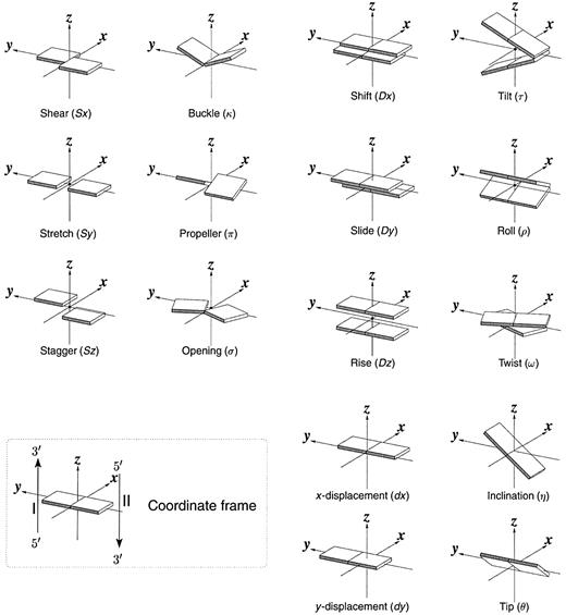
Figure 1. Pictorial definitions of rigid body parameters used to describe the geometry of complementary (or non‐complementary) base pairs and sequential base pair steps (19). The base pair reference frame (lower left) is constructed such that the x‐axis points away from the (shaded) minor groove edge of a base or base pair and the y‐axis points toward the sequence strand (I). The relative position and orientation of successive base pair planes are described with respect to both a dimer reference frame (upper right) and a local helical frame (lower right). Images illustrate positive values of the designated parameters. For illustration purposes, helical twist (Ω_h) is the same as Twist (ω), formerly denoted by Ω (19,20) and helical rise (h) is the same as Rise (Dz).

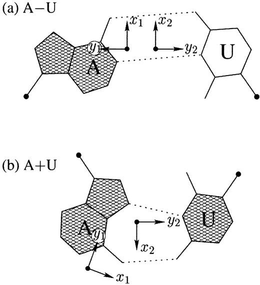
Figure 2. Antiparallel and parallel combinations of adenine (A) and uracil (U) base pair ‘faces’: (a) the antiparallel Watson–Crick A–U pair with opposing faces (shaded versus unshaded) and a 1.5 Å Stretch introduced to separate the two base reference frames; (b) the parallel Hoogsteen A+U pair with base pair faces of the same sense. Black dots on bases denote the C1′ atoms on the attached sugars.

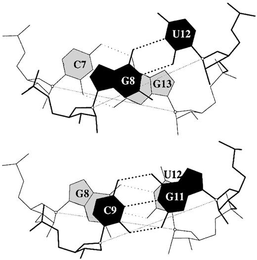
Figure 3. Large Shear of the G–U wobble base pair influences the calculated but not the ‘observed’ Twist. The 3DNA numerical values of Twist, 20° (top) and 43° (bottom), differ from the visualization of nearly equivalent Twist suggested by the angle between successive C1′···C1′ vectors (finely dotted lines). Illustrated dimer steps flank the G(8)–U(12) base pair in the crystal structure of the acceptor stem of E.coli tRNA^Asp (NDB_ID: ar0019) (60).

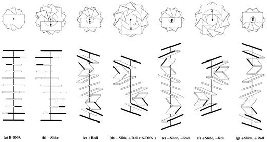
Figure 4. Influence of non‐zero Slide and Roll at sequential dimer steps on overall DNA helical conformation. Images generated with 3DNA building upon the principles of Calladine and Drew (42). The radii of the (dashed) circles in the upper row of images, defined by the loci of points from the helical axes (filled circles) to the base pair origin (open circles), correspond to the x‐displacement. The values of dimeric Twist are adjusted, following equation 4, to keep the helical twist angle at 36°. The A‐like model is highlighted in quotes to emphasize that the structure contains 10 rather than 11 residues per turn.

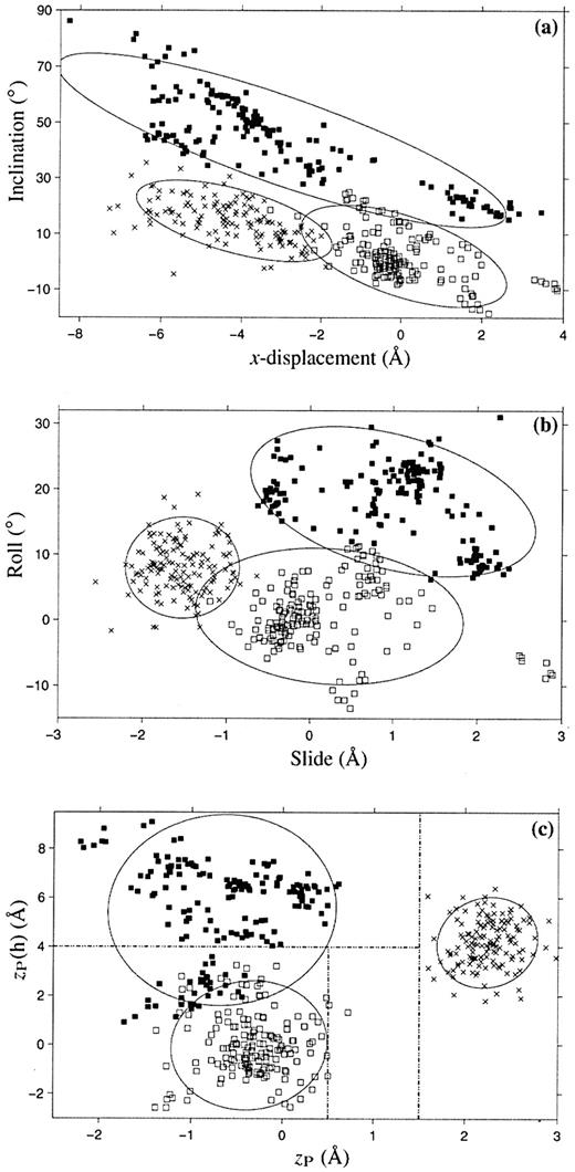
Figure 5. Scatter plots of selected conformational parameters showing the differences among A (× symbol), B (open squares) and TA DNA (filled squares) dinucleotide steps: (a) helical inclination and x‐displacement; (b) dimer step Roll and Slide; (c) projected phosphorus positions, z_P and z_P(h). The contours correspond to ‘energies’ of 2k_BT, i.e.‘2Δθ’ ellipses (17). Dashed lines in (c) illustrate the criteria used in 3DNA to distinguish the three helical forms (see text for details).

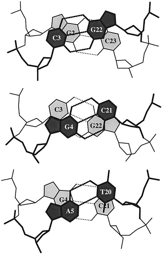
Figure 6. ‘Standardized’ base stacking diagrams of three consecutive dimer steps of the 1.4 Å B DNA structure, d(CGCGAATTCGCG)₂ (NDB_ID: bdl084) (87).

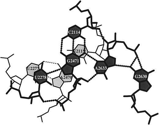
Figure 7. Stacking diagram of a U·G·C·A·G base pentad and a U·A·U triad in the refined structure of the large 50S ribosomal subunit (NDB_ID: rr0033) (3).

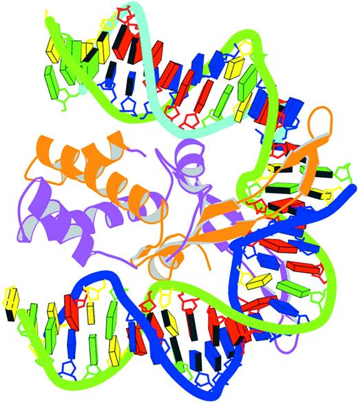
Figure 8. Schematic image of the IHF–DNA complex (NDB_ID: pdt040) (91) shown in the most extended view and color coded according to chain identity and DNA residue type, with the minor groove edges of base pairs shaded.

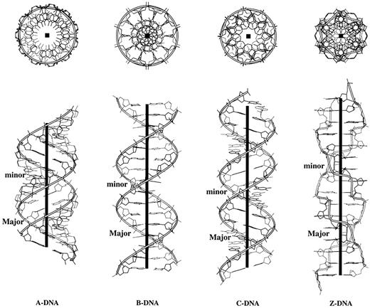
Figure 9. Top and side views illustrating the characteristic features of regular helical structures of A, B, C and Z DNA deduced from representative X‐ray fiber diffraction models (44,46). Ribbons trace the progression of the backbone defined by the phosphorus atoms and the heavy black lines (boxes) represent the helical axes.

Table 1.

Local dimer step parameters and local helical parameters of the regular DNA structures^a shown in Figure 4a–g

	Fig. 4a	Fig. 4b	Fig. 4c	Fig. 4d	Fig. 4e	Fig. 4f	Fig. 4g
Shift (Å)	0	0	0	0	0	0	0
Slide (Å)	0	–2	0	–2	–2	+2	+2
Rise (Å)	3.34	3.34	3.34	3.34	3.34	3.34	3.34
Tilt (°)	0	0	0	0	0	0	0
Roll (°)	0	0	+12	+12	–12	–12	+12
Twist (°)	36	36	34	34	34	34	34
x‐displacement (Å)	0	–3.24	–1.75	–4.81	–1.31	+4.81	+1.31
y‐displacement (Å)	0	0	0	0	0	0	0
Helical rise (Å)	3.34	3.34	3.16	2.51	3.81	2.51	3.81
Inclination (°)	0	0	+19.8	+19.8	–19.8	–19.8	+19.8
Tip (°)	0	0	0	0	0	0	0
Helical twist (°)	36	36	36	36	36	36	36
Helix type	‘B DNA’			‘A DNA’

^aStructures generated with 3DNA using variable Slide, Roll and Twist values in combination with the fixed values of Tilt, Shift and Rise listed above. Twist is adjusted following equation 4 to maintain the helical twist angle at 36°, corresponding to an exact 10 bp helical repeat. For example, a Roll angle of ±12° requires a decrease of Twist to 34° to produce a 36° helical twist.

Table 2.

Characterization of selected DNA structures (average 3DNA parameters)

	Local dimer step parameters				Local helical parametersa				Phosphorus position
Structure	Roll (°)	Twist (°)	Slide (Å)	Rise (Å)	η (°)	Ωh (°)	dx (Å)	h (Å)	zP (Å)	zP(h) (Å)
ud0011 (‘E’)b	2.4	30.3	–1.93	3.32	4.3	30.7	–4.09	3.21	2.45	3.01
adh008 (‘A’)c	5.0	31.4	–1.70	3.31	8.6	32.0	–3.99	3.04	2.55	3.67
ad0023 (‘AB’)d	2.7	31.7	–1.02	3.32	5.6	32.1	–2.45	3.22	1.43	2.29
ad0024 (‘AB’)d	2.5	31.5	–1.05	3.13	5.3	31.8	–2.45	3.05	1.51	2.31
bd0026 (‘AB’)e	3.3	32.5	–1.38	3.27	5.9	32.7	–2.98	3.13	2.46	3.27
A DNAf	8.0 (3.9)	31.1 (4.0)	–1.53 (0.34)	3.31 (0.20)	14.7 (7.3)	32.5 (3.8)	–4.17 (1.22)	2.83 (0.36)	2.24 (0.27)	4.19 (0.93)
B DNAf	0.6 (5.2)	36.0 (6.8)	0.23 (0.81)	3.32 (0.19)	2.1 (9.2)	36.5 (6.6)	0.05 (1.28)	3.29 (0.21)	–0.36 (0.43)	–0.02 (1.32)
TA DNAg	18.2 (5.8)	19.1 (5.0)	0.98 (0.85)	3.30 (0.22)	43.6 (15.6)	27.3 (2.6)	–2.99 (2.79)	2.88 (0.63)	–0.66 (0.63)	5.50 (1.96)

^aSymbols used to designate local helical parameters (η, Ω_h, dx and h) correspond, respectively, to inclination, helical twist, x‐displacement and helical rise.

^bVargason et al. (73).

^cHeinemann et al. (77).

^dVargason et al. (78).

^eNg et al. (75) (GGGCCC region).

^fHigh resolution A and B DNA structures taken from the survey of Olson et al. (20) with standard deviations in parentheses.

^gStructures and dimer steps used to calculate the set of TA‐DNA parameters listed at http://rutchem.rutgers.edu/∼olson/3DNA.

Table 3.

Root mean square deviation (in Å) between rebuilt 3DNA models and experimental DNA structures

Structure	adh026 (86)	bdl084 (87)	pd0001 (88)
All atom	0.52a,c	0.73b,c	0.82b,c
Base atom	0.03	0.02	0.05

^aA DNA backbone conformation based on the fiber model of Arnott (44), where the backbone torsion angles are fixed at the following values: β = 175°, γ = 42°, δ = 79°, χ = –157°.

^bB DNA backbone conformation based on the fiber model of Arnott (44), where β = 136°, γ = 31°, δ = 143°, χ = –108°. The latter value corresponds to the average torsion angle found in high resolution B DNA X‐ray crystal structure (18).

^cPhase angles of pseudorotation of 8° and 154° are used, respectively, to describe the C3′‐endo puckering of the sugar ring in A DNA and the C2′‐endo puckering in B DNA. Backbone torsions α, ϵ and ζ are determined by the assumed positioning of the bases.

Table 4.

Selected features of regular DNA and RNA helical models included in 3DNA

Structure description	Repeating sequence	IDa	Ωh (°)	h (Å)	Shift (Å)	Slide (Å)	Rise (Å)	Tilt (°)	Roll (°)	Twist (°)
A DNA (calf thymus)	generic	1	32.7	2.55	0.00	–1.40	3.30	0.0	12.4	30.3
A DNA	generic	54	32.73	2.56	0.01	–1.49	3.26	–0.1	11.4	30.7
A DNA	ABr5U·ABr5U	2	65.5	5.10	0.00	–1.34	3.25	0.0	12.1	30.5
A DNA (calf thymus)	ATCGGAATGGT	3	360.0	28.03	0.01	–1.27	3.32	–0.1	13.2	30.0
	TAGCCTTACCA
A RNA	A·U	20	32.7	2.81	–0.08	–1.48	3.30	–0.4	8.6	31.6
A′ RNA	I·C	21	30.0	3.00	0.05	–1.88	3.39	–0.1	5.4	29.5
B DNA (calf thymus)	generic	4	36.0	3.38	0.00	0.45	3.36	0.0	1.7	36.0
B DNA (BI nucleotides)	generic	46	36.0	3.38	0.00	0.29	3.37	0.0	2.2	35.9
B DNA	generic	55	36.0	3.39	0.01	0.03	3.40	0.0	–2.4	35.9
B DNA	CG·CG	5	72.0	6.72	0.00	0.84	3.29	0.0	3.5	35.8
B DNA (calf thymus)	CCCCC	6	180.0	16.86	0.31	0.37	3.36	2.9	0.6	35.9
	GGGGG
B′ DNA α (H DNA)	A·T	18	36.0	3.23	–0.08	–0.22	3.23	–2.7	–2.9	35.8
B′ DNA β2 (H DNA β)	A·T	19	36.0	3.23	0.42	–0.76	3.16	–0.6	–5.7	35.6
B′ DNA β2	A·U	37	36.0	3.20	–0.07	–0.55	3.17	–0.3	–2.7	35.9
B′ DNA β1	A·T	38	36.0	3.24	0.13	–0.33	3.22	1.0	–4.3	35.7
B′ DNA β2	AI·CT	39	72.0	6.48	0.02	–0.92	3.15	2.8	–5.3	35.5
B′ DNA β1	AI·CT	40	72.0	6.46	–0.37	–0.45	3.21	–5.7	0.4	35.6
B′ DNA	AATT·AATT	41	144.0	13.54	0.00	0.20	3.39	0.0	–0.3	36.3
DNA β	A·U	43	36.0	3.20	–0.02	–0.69	3.15	0.4	–3.1	35.9
B DNA (Ca salt)	A·T	44	36.0	3.23	0.00	–0.81	3.17	0.0	–3.7	35.8
B DNA (Na salt)	A·T	45	36.0	3.23	–0.02	–0.89	3.16	1.9	–4.0	35.7
B* DNA	A·T	51	31.6	3.22	–0.04	–0.51	3.33	0.2	4.8	31.2
C DNA (calf thymus)	Generic	7	38.6	3.31	–0.01	0.08	3.35	0.0	–5.3	38.2
C DNA (BII nucleotides)	Generic	47	40.0	3.32	0.00	1.75	3.96	0.0	–11.5	38.4
C DNA (LHb)	Generic	53	–38.7	3.29	–0.01	0.89	3.20	0.0	–5.5	–38.3
C DNA	GGT·ACC	8	40.0	3.31	–0.01	1.88	3.53	0.0	–4.4	39.8
C DNA	GGT·ACC	9	120.0	9.94	–0.15	1.30	3.53	1.1	–5.9	39.6
C DNA	AG·CT	10	80.0	6.47	0.00	0.84	3.42	0.1	–7.5	39.8
C DNA	AG·CT	11	80.0	6.47	–0.59	0.86	3.46	–2.0	–8.9	39.2
D DNA	AAT·ATT	12	45.0	3.01	0.00	0.85	3.26	0.0	–9.9	44.0
D DNA	CI·CI	13	90.0	6.13	0.00	1.01	3.40	0.0	–11.2	43.7
D DNA	ATATAT·ATATAT	14	–90.0	18.50	0.00	1.07	3.48	0.0	–13.0	43.3
DA DNA	AT·AT	48	87.8	6.02	0.00	–2.44	3.07	0.0	0.8	43.9
DB DNA	AT·AT	52	90.0	6.06	0.00	1.25	3.42	0.0	–11.2	43.7
L DNA (calf thymus)	GC·GC	17	0.0	10.20	0.00	–0.42	5.08	0.0	0.0	0.0
S DNA (CBGA, RHb)	CG·CG	49	60.0	7.20	0.00	–0.23	3.61	0.0	1.3	30.0
S DNA (CAGB, RHb)	GC·GC	50	60.0	7.20	0.00	–0.18	3.61	0.0	1.3	30.0
Z DNA	GC·GC	15	–60.0	7.25	0.00	1.92	3.59	0.0	0.2	–30.0
Z DNA	As4T·As4T	16	–51.4	7.57	0.00	1.28	3.79	0.0	0.9	–25.7
DNA·RNA hybrid	A·dT	22	32.7	2.56	0.00	–1.66	3.27	0.0	10.8	30.9
DNA·RNA hybrid	dG·C	23	32.0	2.78	0.05	–1.78	3.38	–0.2	8.8	30.8
DNA·RNA hybrid	dI·C	24	36.0	3.13	–0.25	–0.56	3.36	–3.5	9.0	34.7
DNA·RNA hybrid	dA·U	25	32.7	3.06	0.10	–1.25	3.40	–1.1	7.1	31.9
10‐fold (RNA)	X·X	26	36.0	3.01	0.00	–0.67	3.44	0.0	12.6	33.8
11‐fold (RNA)	X·X	27	32.7	2.52	0.00	–1.69	3.20	0.0	10.4	31.0
Symmetric (RNA)	s2U·s2U	28	32.7	2.60	0.02	–1.49	3.30	–0.1	11.4	30.7
Asymmetric (RNA)	s2U·s2U	29	32.7	2.60	–0.30	–1.39	3.26	–7.1	11.2	30.0
DNA triplex	C·I·C	30	32.7	3.16	0.07	–0.97	3.38	2.2	5.9	32.1
DNA triplex	T·A·T	31	30.0	3.26	0.04	–0.99	3.47	1.8	5.0	29.5
RNA triplex (11‐fold)	U·A·U	32	32.7	3.04	0.02	–0.85	3.31	2.4	7.3	31.8
RNA triplex	U·A·U	42	32.7	3.04	0.06	–0.84	3.27	2.5	6.4	32.0
RNA triplex (12‐fold)	U·A·U	33	30.0	3.04	–0.01	–1.03	3.32	2.0	6.1	29.3
RNA triplex	I·A·I	34	30.0	3.29	–0.15	–0.81	3.40	0.9	3.2	29.8
RNA quadruplex	I·I·I·I	35	31.3	3.41	–0.57	–0.36	3.39	0.1	–2.4	31.2
Single‐stranded RNA	eC (O2′ ethyl)	36	60.0	3.16	3.24	–0.70	3.86	–3.2	24.2	55.2

^a3DNA identification numbers: models 1–43 from Arnott and co‐workers (43,44); models 44 and 45 from Alexeev et al. (45); models 46 and 47 from van Dam and Levitt (46); models 48–55 from Premilat and Albiser (47–52).

^bLH, left‐handed helix; RH, right‐handed helix.