Understanding the general feature of microvariability in Kepler blazar W2R 1926+42

Abstract

We analyze the Kepler monitoring light curve of a blazar W2R 1926+42 to examine features of microvariability by means of the “shot analysis” technique. We select 195 intra-day, flare-like variations (shots) for the continuous light curve of Quarter 14 with a duration of 100 d. In the application of the shot analysis, an averaged profile of variations is assumed to converge with a universal profile which reflects a physical mechanism generating the microvariability in a blazar jet, although light-variation profiles of selected shots show a variety. A mean profile, which is obtained by aligning the peaks of the 195 shots, is composed of a spiky-shaped shot component at ± 0.1 d (with respect to the time of the peak), and two slow varying components ranging from −0.50 d to −0.15 d and from 0.10 d to 0.45 d of the peak time. The former spiky feature is well represented by an exponential rise of 0.043 ± 0.001 d and an exponential decay of 0.061 ± 0.002 d. These timescales are consistent with that corresponding to a break frequency of a power spectrum density calculated from the obtained light curve. After verification with the Monte Carlo method, the exponential shape, but not the observed asymmetry, of the shot component can be explained by noise variation. The asymmetry is difficult to explain through a geometrical effect (i.e., changes of the geometry of the emitting region), but is more likely to be caused by the production and dissipation of high-energy accelerated particles in the jet. Additionally, the durations of the detected shots show a systematic variation with a dispersion caused by a statistical randomness. A comparison with the variability of Cygnus X-1 is also briefly discussed.

1 Introduction

Blazars have relativistic jets whose axes are nearly aligned to the line of sight (Blandford & Königl 1979; Antonucci 1993). In principle, the timescales of brightness variations in blazars are related to the sizes of the emitting regions and the speeds of motion in relativistic jets. Variations, however, have a variety of timescales ranging from minutes to decades. The power spectrum density (PSD) of a blazar can be fitted by a power law, which means that variations of blazars follow a noise-like behavior (Kataoka et al. 2001). Brightness variations of blazars could be affected by a variety of physical conditions: size and speed of the emission region, changes in magnetic field, etc. Shorter-timescale variations can reflect physical processes in the inner emitting regions of a jet without any direct relation to the other, more slowly varying component(s). The study of short-timescale fluctuations is therefore important towards the investigation of the origin of variation in blazar jets.

Blazars show variations that have a timescale of less than one day, termed “microvariability.” Such microvariability has been reported over wide ranges of wavelengths from radio (Quirrenbach et al. 1992) to optical (Carini et al. 1990), X-ray (Kataoka et al. 2001), and TeV bands (Aharonian et al. 2007). The Fermi space telescope scans the entire γ-ray sky every three hours, and has detected flares, large-amplitude variations, in a number of blazars (Abdo et al. 2011). Saito et al. (2013) reported that a few flares in PKS 1510−089 exhibited asymmetric profiles. Nalewajko (2013), however, reported that there was a great variety of flare shapes and duration among 40 flares that he studied, so that the flares cannot be described by a simple rise and decay. It is not easy to extract detailed features of flare-like variations in the γ-ray band, because the time required to measure the γ-ray flux with Fermi and AGILE is usually longer than three hours, except for a detection of minute-timescale γ-ray variation by operating a special pointing mode to optimize the exposure for 3C 279 (Ackermann et al. 2016), since the number of detected photons is limited. A statistical study of a sizeable number of variation events with higher time resolution and with good photon statistics is needed to extract the general features of microvariability in an effort to understand the underlying physics of relativistic jets.

The blazar W2R 1926+42 has a synchrotron spectral energy distribution (SED) that peaks at a frequency of below 10¹³ Hz. The object is classified as a low-frequency peaked BL Lac object at a redshift z = 0.154 that is estimated from two absorption lines in the spectrum of its host galaxy (Edelson & Malkan 2012). Edelson et al. (2013) also reported numerous flares on timescales as short as 1 d in the Kepler light curve with 30-min time-sampling in Quarters 11 and 12. Continuous optical monitoring of W2R 1926+42 with denser (1 min) time-sampling by Kepler (Borucki et al. 2010) in Quarter 14 detected considerable microvariability of the flux.

We wish to stress here that it is of limited use to examine a variety of individual shapes of time profiles of flux variations. In order to gain physical insight, it is more useful to examine the average properties. Therefore, in this paper we adopt a stacking analysis, so-called “shot analysis”, to obtain a mean profile of rapid variations. The paper is organized as follows. Details of the Kepler observed light curve and its PSD are described in section 2. The methods of time-series analysis, shot analysis, bootstrap method, and Monte Carlo method, are described in section 3. Observational features of the mean profile of rapid variations and its validation by a Monte Carlo simulation are reported in section 4. We then discuss the mechanism of variations as derived from general features of the rapid fluctuations in section 5. Several concluding remarks based on our results are provided in section 6.

2 Observation and light curve

2.1 Kepler data

Kepler monitored over 100000 objects in the Cygnus region, obtaining continuous light curves with two timing settings, long (30 min) and short (1 min) integrations. W2R 1926+42 is listed in the Kepler target list. A continuous light curve with the long cadence has been obtained since Quarter 11. In Quarter 14, the object was monitored in the short cadence mode for 100 d. We have produced the calibrated “SAP_FLUX” light curve with 1-min time resolution by the automated Kepler data processing pipeline (Jenkins et al. 2010).

2.2 Light curve

Figure 1 shows an optical light curve of the object obtained by Kepler. The blazar displayed violent variability over various timescales ranging from several tens of minutes to over 10 days during this monitoring. The light curve is composed of not only large-amplitude, long-term variations such as that ranging from JD 2456150 to 2456160, but also numerous flare-like variations with timescales <1 d. These rapid variations exist throughout this entire monitoring period. A variety of profiles is apparent in these rapid variations. Figure 2 shows five examples of the rapid variations (all profiles of rapid variations are provided in supplementary figure 1).

Fig. 1.

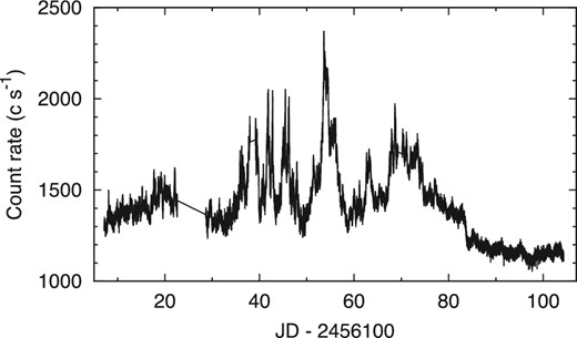
Light curve obtained by the Kepler spacecraft over the entire Quarter 14 period. The object was monitored for 100 d with 1 min time resolution.

Fig. 2.

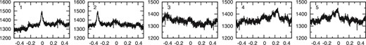
Examples of rapid variations. The peak times of these variations are shown as the origins. The vertical axis corresponds to the count rate. These variations are numbered in supplementary table 1 as shots. See supplementary figure 1 for all profiles of detected variations.

2.3 Power spectrum density

PSD analysis is one of the best ways to quantify time-series data. We calculate the PSD of the Kepler light curve to explore whether there is a characteristic timescale or not. We separate the observed light curve into five epochs, each with a duration of approximately 20 d, and calculate PSDs at each epoch. In doing so, we implicitly assume that the PSD is stationary throughout the entire range of the light curve. We average 20 continuous power estimates and calculate the standard error on a logarithmic scale (Papadakis & Lawrence 1993). The standard error would contain the systematic error affected by the variation of PSDs in each epoch.

Figure 3 shows the PSDs calculated from the observed light curve. We calculate the best-fitting power-law function, adding a constant value in panel (A), by evaluating the goodness-of-fit with a χ² test;

\begin{eqnarray} {\chi }^{2}=\sum \left(\frac{P_{\rm obs}-P_{\rm expect}}{{\sigma }_{\rm err}}\right)^{2}, \end{eqnarray}

(1)

where P_obs and P_expect are the observed and expected PSDs, and σ_err is the uncertainty in the observed PSD. Residuals in panel (B) indicate a discrepancy at lower frequencies. We add a squared Lorentzian component to the power-law function as;

\begin{eqnarray} P_{\rm model}(f)=A f^{-\alpha } + \frac{B}{[1+(f/f_{\rm br})^{2}]^{2}} + C, \end{eqnarray}

(2)

where α is a spectral index and f_br is a break frequency. The best-fitting function is shown in panel (C). Dashed lines represent individual terms of function (2). The goodness-of-fit for the best-fitting function improves over that for the best-fitting power-law. The existence of this curvature has already been pointed out (Edelson et al. 2013; Mohan et al. 2016).

Fig. 3.

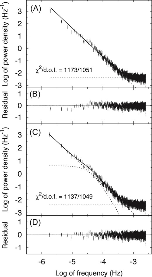
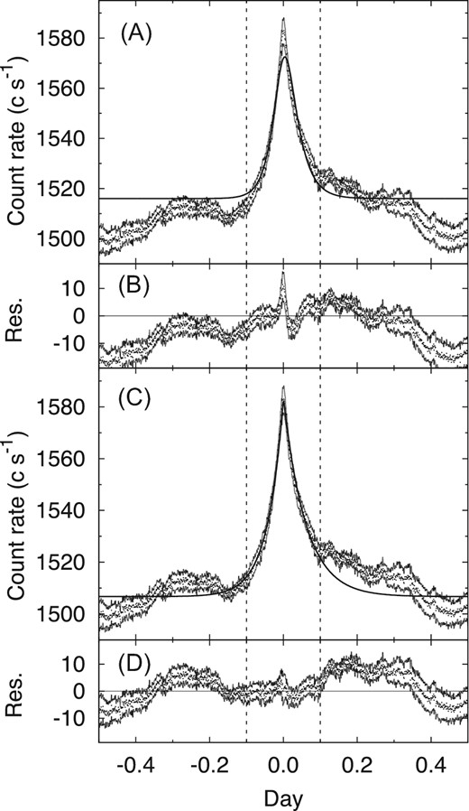
Power spectrum densities calculated from the observed light curve. Panels (A) and (B) show the observed PSD, the best-fitting power-law function and constant, and its residuals. Panels (C) and (D) show the PSD, the best-fitting function of (2), and its residuals. Dashed lines in panel (A) and (C) show individual components of the best-fitting functions. Goodnesses of fit, χ² per degrees of freedom (d.o.f), are also indicated.

The curvature in the observed PSD indicates that the light curve has the characteristic timescale related to the break frequency of the PSD. The break frequency of the best-fitting function (2) is |$4.1^{+0.6}_{-0.5} \times 10^{-5}\:$|Hz, corresponding to f_br = (2πτ_br)⁻¹, with τ_br = 0.045 ± 0.006 d, for time-symmetry exponential shots (Negoro et al. 2001).

If the variation is caused by flickering or 1/f fluctuation, there is no physical significance in the rapid variation associated with the higher-frequency PSD component, because a higher-frequency variation is generated as a result of a longer-timescale fluctuation. This fluctuation, however, should not have a characteristic timescale. The observed characteristic timescale indicates the underlying physics associated with that timescale.

3 Time-series analysis techniques

3.1 Shot analysis

Frequency-domain (e.g., PSD) analyses are easy to perform, but are difficult to relate to physical mechanisms. One would prefer a time-domain study that is useful for investigating the physical mechanisms of flare-like variations. This is, however, not easy to accomplish, especially when the photon statistics are insufficient, because it is difficult to perform detailed studies on a section of the observed data with high observational uncertainties. Additionally, observed flares in blazars usually have a variety of shapes (Nalewajko 2013). Thus, it is difficult to extract common features of blazar flare-like variations by studying only individual events.

Shot analysis proposed by Negoro, Miyamoto, and Kitamoto (1994) is one of the best ways to study the common features of variation. The shot analysis calculates the mean of flare-like variation events by stacking these events. An influence in the mean by respective features of individual events should be decreased by applying this stacking technique. Thus, the mean can be reduced the influence of the variety of shapes at individual variations as well as the variations caused by the observational uncertainty. Here, the averaged profile of flare-like variations is assumed to converge with a universal one. In other words, if samples of flare-like variations are innumerable, the average profile should be coincident with the universal one reflecting general features of flare-like variations. If the variability has the characteristic timescale, the phase information can be extracted from the mean profile of the variations associated with the characteristic timescale, regardless of whether the variability is attributed to continuous or discrete processes. Hence we can investigate the physical mechanism associated with the characteristic-timescale variation from the mean of flare-like variation events.

We apply the shot analysis to the light curve of W2R 1926+42 obtained by Kepler in order to generate a mean profile of flare-like rapid variations and to study its general features without being distracted by features specific to individual events. We adopt the following procedures to select rapid variations.

• Estimate the observational uncertainty in the light curve.

• Select rapid variations from the light curve as representatives of flaring events.

• Approximate a long-term slow-varying component with a polynomial function in each candidate.

• After subtracting the long-term components, select the rapid variations with variation amplitudes that are four times larger than the observational uncertainty.

We define these representative variations as shots. After identifying the shots, we stack them aligning their peaks, and calculate the mean profile. An example of shot detection is shown in sub-subsection 4.1.1.

The observational uncertainty is estimated as follows. There are two possibilities for varying the observed brightness: intrinsic variation of the object, and variation from observational uncertainty. The latter can be dominant over the former within a short time period. We calculate differences of fluxes between two neighboring points as ΔF(t_n) = F(t_n+1) − F(t_n), where F(t_n+1) and F(t_n) are the (n + 1)th and nth photon fluxes at those times. We define the standard deviation σ of ΔF(t_n) as the observational uncertainty, σ = 17.15 c s⁻¹. At this time, we do not include values of ΔF(t_n) with long time differences (>2 min) to avoid contaminations of data that might have components with large intrinsic variations because the light curve often has long blank periods caused by instrumental limitations.

Rapid variations are often superposed on long-term variations in the light curves of blazars (Sasada et al. 2008). We approximate the long-term baseline component by a second-order local polynomial that fits the trend of the light curve when the rapid fluctuations are ignored. We identify a shot when the estimated amplitude of the rapid variation, without the contribution of the baseline component, is larger than our threshold criterion, >4σ.

The peak time of the shot is defined as the time of maximum flux in the light curve after subtraction of the baseline component. We calculate the mean profile of detected shots by stacking numerous shots after aligning their peaks. Here, we average the shots without subtracting the baseline components. The final shape of the mean profile does not depend on the existence of the baseline component in each shot, since the baseline component of the mean profile should be smoothed and asymptotically close to constant in time.

3.2 Non-parametric bootstrap method

The bootstrap method that we employ determines the distribution of an estimator or test statistic by resampling either the data or a model derived from the data (Efron & Tibshirani 1979; Efron 1994). The bootstrap method first provides an approximation to the probability distribution of the estimator in the detected samples. Then, the coverage probabilities of confidence intervals can be estimated from the probabilities of the distributions. We apply a non-parametric bootstrap method to the dataset of shots, and try to estimate a systematic uncertainty and a confidence interval of the mean profile of shots, as well as confidence intervals of best-fitting parameters of the function that reproduce the mean profile of resampled shots.

We identify 195 shots from the Kepler monitoring light curve of W2R 1926+42, as presented below in subsection 4.1. We resample these shots to produce 195 resampled shots. We then calculate the mean profile using these resampled shots (hereafter, resampled mean profile). We produce 10⁴ resampled mean profiles with different resamplings by following this procedure.

The best-fitting parameters of the function representing the shots can be calculated from each resampled mean profile. Confidence intervals of parameters of the function can be evaluated from the probability distributions of the best-fitting parameters calculated from each resampled mean profile.

3.3 Monte Carlo simulation of noise variation

Time-series analyses in past studies have found that blazar variations are similar to aperiodic red noise, meaning that variations on longer timescales have greater power. We evaluate the characteristics of noise process by applying the above shot analysis. We then compare the characteristics with the observed features of the mean profile of shots, and examine the difference between the shot features estimated from the noise process and the observed light curve.

We adopt a Monte Carlo method that applies the inverse Fourier transform of the observed PSD to represent aperiodic noise-like linear time-series with an additive sine model (Timmer & König 1995). At this point, we assume the best-fitting model of function (2) when the observed PSD is used as the input. Furthermore, we adopt a generation process of non-linear time-series with a multiplicative sine model proposed by Uttley, McHardy and Vaughan (2005). We actually calculate a simulated linear time-series by using a fast Fourier transform technique, with the PSD including random fluctuations. We then convert this to a simulated non-linear time-series through an exponential transform.

The time resolution of a simulated variation is 60 s, and its duration is 100 d (corresponding to the estimations of 144000 points). The mean and standard deviation, μ_l and σ_l, of the generated simulated linear variation, l(t), is adjusted to that of the observed light curve (equal to 1413.7 c s⁻¹ and 197.3 c s⁻¹). To calculate a simulated non-linear variation, x(t), first the generated simulated linear variation is offset to μ_l = 0. Next, its variation is converted through an exponential transform. Then, the mean and standard deviation of its non-linear variation, μ_x and σ_x, are represented as

\begin{eqnarray} {\mu }_{x}={\rm exp}\left[\frac{1}{2}{\sigma }_{l}^{2}\right], \end{eqnarray}

(3)

\begin{eqnarray} {\sigma }_{x}={\rm exp}\left[{\sigma }_{l}^{2}\right]\left( {\rm exp}\left[{\sigma }_{l}^{2}\right] - 1 \right). \end{eqnarray}

(4)

The fractional rms, σ_frac, is defined as the standard deviation divided by the mean, which corresponds to a skewness of x(t). This fractional rms is characterized by equations (3) and (4) as

\begin{eqnarray} {\sigma }_{\rm frac}=\sqrt{{\rm exp}\left[{\sigma }_{l}^{2}\right]-1}. \end{eqnarray}

(5)

In this simulation, we assume that σ_frac of the simulated non-linear variation is equal to 0.64. Finally, the mean and standard deviation of x(t) are adjusted to the observed values.

We select local peaks of the simulated linear variation. Mean profiles of local peaks in the simulated linear and non-linear variations are calculated from 195 peaks, the same as the number of detected shots (see sub-subsection 4.1.2 below).

4 Results

4.1 Shot analysis

The PSD analysis reveals that the variability of W2R 1926+42 has the characteristic timescale as the curvature of the PSD. This indicates the physical background associated with the variation timescale. We perform the shot analysis to the Kepler light curve to extract phase information of variation with the characteristic timescale of the object.

A large number of hour-scale episodes of rapid variations are detected in the light curve. We generate the mean profile of shots that satisfy the definition mentioned in subsection 3.1 to extract general features of the rapid variation.

4.1.1 Example of shot detection

Many temporal surges in flux are seen in the light curve. We select these surges and discriminate against large-amplitude variations according to the criteria given in subsection 3.1. Figure 4 shows an example of shot detection. Only the peak at JD 2456108.09 can be identified as a shot. We estimate the amplitude of the variation by subtracting the best-fitting polynomial baseline component of the light curve. Small-amplitude surges seen on JD 2456107.86 and 2456108.40 do not satisfy the criteria of shots. We detect 195 shots from the entire light curve. All shots are displayed in the supplementary figure 1.

Fig. 4.

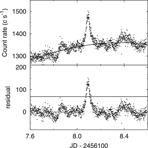
Example of shot detection. The top panel shows a light curve with a detected shot and a polynomial function approximating a long-term baseline component underlying the shot shown as solid line. The bottom panel shows the light curve after subtraction of the best-fitting polynomial function. The solid line indicates the threshold for detecting shots.

4.1.2 Mean profile of shots

We calculate the mean profile of 195 detected shots. Figure 5 shows the mean profile of shots. The plot omits the count rate at the peak time (t = 0), since positive fluctuations of the counts at this time are summed systematically (Negoro et al. 1994).

Fig. 5.

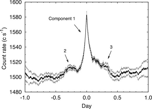
The mean profile of detected shots. Dotted lines show standard deviations of the mean profile. These standard deviations are calculated from mean profiles of shots detected at light curves which are separated six epochs. See the text for details.

There are three main components in the mean profile: a spike-like component at  ± 0.1 d (component 1), and slowly varying components ranging from −0.50 to −0.15 d and from 0.10 to 0.45 d (component 2 and 3, respectively). The increase and decrease of component 1 are well reproduced by an exponential rise and decay. The peak is spiky but smoothly connected from the rise to decay phases.

There is a possibility that shots evolve with time. The systematic uncertainty of the mean profile of shots should include the influence of the time evolution of shots. To estimate the systematic uncertainty, we separate the light curve into six epochs: (1) JD 2456106–2456125, (2) 2456128.6–2456143.6, (3) 2456143.6–2456158.6, (4) 2456158.6–2456173.6, (5) 2456173.6–2456188.6, and (6) 2456188.6–2456205. Individual mean profiles are calculated from shots located in each epoch. We estimate variances of the mean profiles in each time step. We then calculate the standard deviation of the weighted mean, because the number of shots in each epoch is different. Here we normalize fluxes of individual mean profiles within  ± 1 d to average fluxes over all of the mean profiles, since components 2 and 3 are distributed within ±1 d.

Figure 5 shows the mean profile of shots and calculated standard deviations of the weighted means at each time step. The amplitudes of components 2 and 3 are larger than the standard deviations. Therefore, components 1, 2, and 3 of the mean profile of shots can be regarded as real phenomena, not artifacts of the systematic uncertainty of the sampling of shots.

4.1.3 Model for component 1 of the mean profile

Component 1 is distributed around the peak time of mean profile of shots. General features of shots can be extracted from this component. First, we characterize the shape of component 1 to a function proposed by Abdo et al. (2010):

\begin{eqnarray} F(t) = F_{0}\,[e^{-t/T^{\prime }_{\rm r}}+e^{t/T^{\prime }_{\rm d}}]^{-1} + F_{\rm c}, \end{eqnarray}

(6)

where |$T^{\prime }_{\rm r}$| and |$T^{\prime }_{\rm d}$| are variation timescales of the rise and decay phases, F_c represents a constant level underlying component 1, and F₀ measures the amplitude of the shot.

We evaluate the goodness-of-fit of this function with a χ² test. The standard deviation of the weighted mean between six mean profiles of shots detected from individual epochs is adopted as an estimate of the systematic error, σ_err, to calculate the χ² of component 1. The goodness-of-fit of component 1 by function (6) is χ² = 218.7.

For comparison, we apply another function (cf. Negoro et al. 1994):

\begin{eqnarray} F(t) = \left\lbrace \begin{array}{l{@}{\quad}l}F_{0}\, e^{|t|/T_{\rm r}} + F_{\rm c}; & (t < 0) \\ F_{0}\, e^{-|t|/T_{\rm d}} + F_{\rm c}; & (t > 0), \end{array} \right. \end{eqnarray}

(7)

where T_r and T_d are e-folding times of the rise and decay, and F_c and F₀ are the same as in the case of function (6). Since the number of degrees of freedom is equal to that in the case of function (6), we can compare values of χ² between the best-fitting functions of (6) and (7) directly. The goodness-of-fit of function (7) is χ² = 52.6, which is better than that of function (6). Figure 6 shows the applied functions with the best-fitting parameters superposed on the mean profile and its residuals. Although function (6) shows obvious residuals during the peak time, as shown in panels (A) and (B) of figure 6, the residuals in the case of function (7) are suppressed, as shown in panels (C) and (D). This indicates that the mean profile is more spiky than expected from function (6). Thus, function (7) is better suited than function (6) to represent component 1 of the mean profile of shots.

Fig. 6.

Best-fitting functions superposed on the mean profiles of shots. Panels (A) and (C) show the mean profile of shots and the best-fitting functions (6) and (7). Panels (B) and (D) show residuals between the mean profiles and the estimated best-fitting functions. Dashed lines show the fitted range.

The best-fitting parameters of function (7) are shown in table 1. The best-fitting e-folding times of the rise and decay phases, at 0.043 d and 0.061 d, are different. We note that the average of these timescales, 0.052 ± 0.003 d, is consistent with the variation timescale calculated from the break frequency of the PSD within 1σ confidence level (subsection 2.3). This result indicates that component 1 corresponds to the curved feature seen in the observed PSD.

Table 1.

Parameters of best-fitting function (7) to component 1 of the mean profile of shots.

	Best-fitting value
T  r (d)	0.043 ± 0.001
T  d (d)	0.061 ± 0.002
F  0 (c s−1)	76.7 ± 0.6
F  c (c s−1)	1506.7 ± 0.8

Apparently, the rise timescale of the shot in figure 6 is slightly shorter than that of the decay. Is this difference statistically significant? To answer to this question, we calculate confidence intervals of the parameters of function (7) and the ratio between the rise and decay e-folding times.

We estimate the rise and decay timescales from the best-fitting functions (7) of six mean profiles of shots selected from different epochs. The rise and decay timescales are different in epochs; 0.077 and 0.124 (epoch 1), 0.027 and 0.041 (epoch 2), 0.029 and 0.054 (epoch 3), 0.077 and 0.127 (epoch 4), 0.091 and 0.090 (epoch 5), and 0.094 and 0.236 (epoch 6), respectively. These timescales indicate that the characteristic timescale is variable in time. We calculate ratios of the rise to decay timescales to understand how asymmetric the mean profiles are. Most of the ratios are less than 1, and only one profile is approximately equal to unity. These ratios are distributed from 0.40 to 1.01. We calculate the weighted mean of the ratios of timescales and its standard deviation associated with the number of shots as 0.63 ± 0.11. This indicates that the profiles of shots strongly tend to show a fast-rise and slow-decay feature.

The mean profile of shots may have a deviation associated with the variation of individual shapes of 195 shots. To verify the effect of this deviation to the asymmetry of the mean profile, we evaluate the difference between the rise and decay e-folding times by using the non-parametric bootstrap method as mentioned in subsection 3.2. We generate 10⁴ resampled mean profiles, and calculate the best-fitting parameters of function (7) for component 1 of each resampled mean profile. The confidence levels of parameters can be estimated from distributions of best-fitting parameters. Figure 7 shows distributions of T_r and T_d. This clearly shows that these parameters are differently distributed.

Fig. 7.

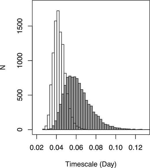
Histograms of T_r (white) and T_d (gray) of the best-fitting function (7). The best-fitting parameters are calculated from 10⁴ resampled mean profiles generated by the non-parametric bootstrap approach. See text for details.

We apply the Wilcoxon rank-sum test, which is a non-parametric significance test (also referred to as the Mann-Whitney U-test), to the distributions of T_r and T_d (Wilcoxon 1945; Mann & Whitney 1947). Since the p value of the Wilcoxon rank-sum test is less than 10⁻¹⁵, we confirm that median values of the distributions of T_r and T_d calculated from the detected shots are clearly different. For these evaluations, component 1 in the mean profile is asymmetric in this case of 195 detected shot samples.

4.1.4 Amplitude dependence of mean profiles

Since rapid variations observed in the light curve have various amplitudes, the shot detection is defined with a threshold of >4σ. If the profile of rapid variations depends on its amplitude, the calculated mean profile of shots does not reflect general features of the rapid variations. We separate detected shots into four groups based on amplitudes of 4–5.7σ, 5.7–7σ, 7–9.5σ, and over 9.5σ, and verify the amplitude dependence of the shot profile by comparing the profiles of four groups. Figure 8 shows mean profiles of shots with different amplitudes. All profiles have component 1 within ± 0.1 d of the center. These shot profiles do not have any clear trend associated with their amplitudes, except for the amplitudes of component 1, although these profiles have local features that are caused by the limited number of shot samples. All the ratios of the rise to decay timescales in each profile are less than unity (average and standard deviation of these ratios are 0.69 and 0.18 respectively). These results indicate that the mean profile of 195 shots reflects the general nature of the rapid variations, and the asymmetric feature of the mean profile of shots is not an artificial one caused by the amplitude dependence of shots.

Fig. 8.

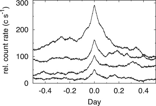
Mean profiles of shots with different amplitudes. From bottom to top, profiles are calculated from shots with amplitudes of 4–5.7, 5.7–7, 7–9.5, and over 9.5σ, respectively. Each profile is offset for clarity. The vertical axis shows the relative count rate.

4.2 Shot durations

The detected shots displayed a variety of shapes. It is, however, assumed that the averaged shape of the shots converges to the exclusive shape in the shot analysis. If the averaged shape of the shots converges to the unique shape which reflects the general feature of the shots, the durations of the shots would distribute around its characteristic time. To validate the convergence of the shot shapes, we calculate the widths of e-folding rise and decay times in each shot as durations, and investigate their distribution.

We calculate the shot durations as follows. First, the baseline component under a shot is approximated by the second-order polynomial function. Here we set a fitting region for this approximation in each shot. Secondly, the approximated baseline component is subtracted from the light curve to estimate an amplitude of the shot. Thirdly, e-folding timescales in the rise and decay phases are calculated from the subtracted light curve. Finally, these timescales are summed as a duration of the shot. In some cases of shots, other variation components are contaminated to the shot components. The e-folding timescales should be longer for the contamination. Then, we extrapolate by linear regression to expect the buried shot component and estimate the e-folding time from the expectation.

4.2.1 Distribution of durations

Figure 9 shows a distribution of shot e-folding durations. Estimated durations of shots range from 0.018 to 0.71 d, with a mean of 0.122 and a standard deviation of 0.097 d. In table 2, the number, peak date, amplitude, duration, and rise and decay times in each shot are given (data for all shots are provided in supplementary table 1). The durations are distributed with a characteristic time, and its distribution can be represented by the log-normal function:

\begin{eqnarray} f(x)=\frac{1}{\sqrt{2{\pi }}}{\rm exp}\left[-\frac{({\rm log}x - {\rm log}{\mu })^{2}}{2{\sigma }^{2}}\right] \end{eqnarray}

(8)

where μ and σ represent the mean and variance of the distribution (Negoro & Mineshige 2002). The distribution is evaluated to the log-normal function by the Kolmogorov and Smirnov test (with a p value of 0.53). The best-fitting log-normal function is shown as a solid line in figure 9.

Fig. 9.

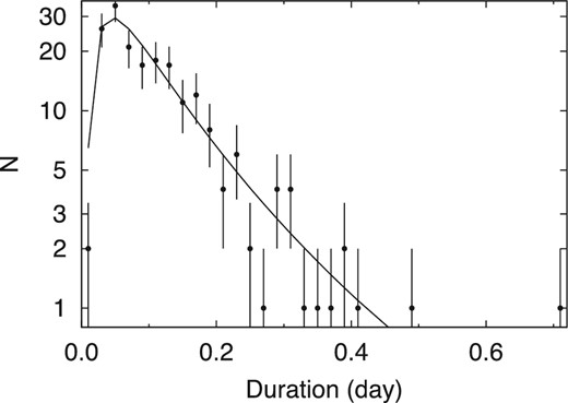
Distribution of estimated shot durations. Solid line shows the best-fitting log-normal distribution.

Table 2.

Amplitude and e-folding timescales of shots.*

No.	Date	Amplitude	Duration	Rise time	Decay time
1	8.0924	152 ± 17	0.042 ± 0.006	0.018 ± 0.005	0.024 ± 0.001
2	8.4207	82 ± 17	0.096 ± 0.035	0.057 ± 0.017	0.039 ± 0.018
3	8.8232	71 ± 14	0.090 ± 0.035	0.042 ± 0.016	0.048 ± 0.020
4	9.6917	69 ± 14	0.068 ± 0.034	0.039 ± 0.019	0.029 ± 0.015

* Columns: 1 – number, 2 – peak date (JD 2456100), 3 – amplitude (c s⁻¹), 4 – duration (d), 5 – rise time (d), 6 – decay time (d).

The mean of these durations is slightly larger than the duration (best-fitting T_r plus T_d of 0.104 d) of the mean profile of shots. This can be caused by the large-side tail of the distribution of durations as evidence that the median value of the distribution of 0.098 d is similar to the value of T_r plus T_d of the mean profile.

If the durations arise following a random manner or a provability distribution of a power-law function, the distribution should be flat or without any peaks. If the distribution of durations follows the power-law function with a lower cutoff, there is a physical background for the lower cutoff of this distribution, because the minimum duration of 0.018 d is clearly larger than the cutoff caused by the time-resolution limit of several times of 0.00068 d (= 1 min). Thus, the duration at the peak of the distribution is produced by the physics of the jet rather than the time-resolution limit. Therefore, the distribution of the durations implies that the averaged shape of shots is converged to the typical one which reflects the physical background of the object.

4.2.2 Time evolution of variation timescales

Figure 10 shows the light curve and the time series of estimated durations in the detected shots together with the average and standard deviation of each 10-point duration set in a logarithmic scale. The averaged durations show a systematic variation with time. To validate that this systematic variation is not a result of a random manner, we calculate a χ²/d.o.f of these averaged durations to the best-fitting constant value in the logarithmic scale. Here, we assume that durations in each 10-point set are randomly distributed according to a log-normal probability density. Therefore, the standard deviation of each 10-point duration set is used as the σ_err in equation (1). The calculated χ²/d.o.f is equal to 52.3/19, which corresponds to a p value of 1.04 × 10⁻⁵. This result indicates that the averaged durations are variable with time. Thus, the shot events are associated with each other, not randomly distributed.

Fig. 10.

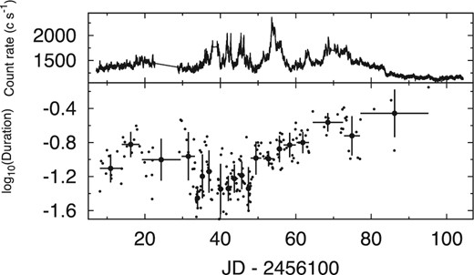
Time series of shot durations. The Kepler light curve (upper panel) and the time variation of the durations are displayed. The time series of averaged durations is also shown in the bottom panel.

4.3 Validation of shot features by Monte Carlo simulation

In subsection 4.1, we found general features of rapid variation in the object by applying shot analysis to the Kepler light curve. It is not known, however, whether the general features result from the natures of the AGN jet physics or statistics. The observed general features extracted from the mean profile of shots should be separated into these two categories by using the Monte Carlo method. We evaluate the stochastic features of the simulated noise variation generated by the Monte Carlo method (see subsection 3.3) by applying the shot analysis, and compare these features with the observed ones. Then we determine the causes of the observed features.

Figure 11 shows the mean profiles of local peaks selected from simulated linear and non-linear variations, and displays the observed mean profile of shots for comparison. All profiles clearly have peak signals distributed about the origin. The rise and decay phases of the mean profiles calculated from both the simulated linear and non-linear variations are consistent with the exponential rise and decay forms, which are also consistent with the observed ones. Durations of the peak component in the mean profiles of local peaks in the linear and non-linear variations are approximately equal to the duration of component 1 ( ± 0.1 d). This similarity can be caused by having the observed and reference PSDs having the same break frequencies, equal to 4.1 × 10⁻⁵ Hz.

Fig. 11.

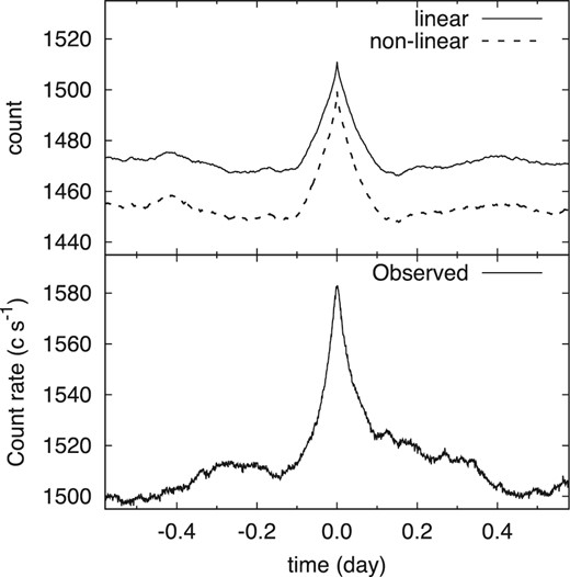
Mean profiles of local peaks calculated from simulated linear and non-linear variations, and the observed mean profile of shots. The mean profiles in the top panel are calculated from 195 local peaks selected from a simulated linear (solid line) and non-linear (dashed line) variations. The observed mean profile of shots in the bottom panel is shown for comparison.

Averages of e-folding times in the rise and decay phases of profiles calculated from the simulated linear and non-linear variations are approximately equal to 0.084 (rise in linear), 0.084 (decay in linear), 0.078 (rise in non-linear), and 0.078 d (decay in non-linear), respectively. Standard deviations of rise and decay e-folding times calculated from 10³ simulated linear and non-linear variations are almost the same value, 0.015 d. The timescales in both the linear and non-linear cases are longer than those of the observed mean profile. Furthermore, the rise and decay timescales of profiles of the simulated variations are almost the same. That is, the profiles are symmetric, while component 1 of the observed mean profile contains some asymmetry.

We evaluate whether the observed asymmetry can be explained by fluctuations in the simulated rise and decay timescales of local-peak profiles calculated from linear and non-linear variations. First, we generate 10³ mean profiles of local peaks of simulated variations with the linear and non-linear processes. Secondly, the ratio between the best-fitting e-folding times of the rise and decay phases is estimated from each mean profile. Finally, we compare the probability distributions of those ratios calculated from the 10³ simulated linear and non-linear variations with the observed ratio between the e-folding times of rise and decay phases. Figure 12 shows histograms of 10³ ratios between the rise and decay timescales of mean profiles in the cases of both the linear and non-linear processes. These are clearly distributed about unity. This result indicates that the rise and decay timescales calculated from linear and non-linear noise variations should be the same. According to the Student's t-test, the ratio of timescales in the observed mean profile (= 0.70) is clearly different from the median values of ratios calculated from these simulated mean profiles (the p values are both less than 2.2 × 10⁻¹⁶). Thus, the difference between the rise and decay timescales observed in the mean profile of shots is caused by a physical phenomenon, not the result of the stochastic noise variation generated by the Monte Carlo method using the PSD with a break frequency.

Fig. 12.

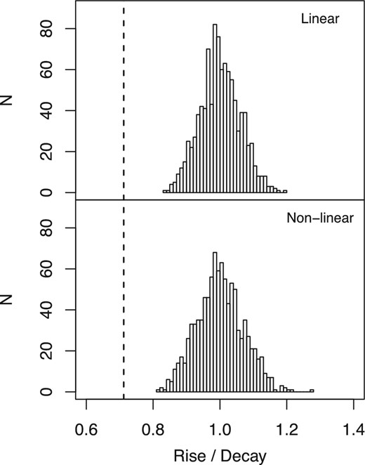
Histograms of 10³ ratios between rise and decay timescales. The rise and decay timescales are calculated as e-folding times of mean profiles of simulated linear (top panel) and non-linear (bottom panel) variations. Dashed lines show the observed ratio of rise and decay timescales.

5 Discussion

5.1 Origin of rapid variations

It is poorly understood whether rapid variations of blazars are intrinsic phenomena or an apparent occurrence caused by a geometrical effect, such as the precession of a jet axis. There are several models that explain flux variations as apparent rather than as caused by changes in the intrinsic luminosity. This can occur, for example, if the Doppler factor varies owing to changes in the viewing angle in a bent jet (Villata & Raiteri 1999) or to the effects of gravitational lensing (Chang & Refsdal 1979). Such models, however, predict that the averaged variation profile is approximately symmetric in a simple geometry, because the Doppler factor or lensing should change symmetrically. In other words, rise and decay timescales of an average profile of rapid variations should be roughly equal, whereas the estimated rise and decay timescales are different. Thus, rapid variations cannot generally be explained by these models, but rather as intrinsic phenomena. If particles are accelerated in the jet, the number of higher-energy particles are increased in the emitting region during rapid variations, where they dissipate their energies. The flux-variation profile should be asymmetric in this particle-acceleration scenario, because the rise and the decay of the brightness are caused by different mechanisms: particle acceleration and dissipation processes. Therefore, rapid variations are plausibly explained by the particle-acceleration scenario.

5.2 Values of the magnetic field and Doppler factor

The mean profile of shots calculated by the shot analysis represents the variation with the characteristic timescale. This reflects an “averaged” situation of emitting regions of shots. We can estimate the common physical values of emitting regions from the mean profile of shots.

It is plausible that the dissipation of high-energy particles during rapid variation is caused by a synchrotron cooling. The timescale for this process, τ_syn, can be related to the decay timescale T_d; τ_syn = T_d/(1 + z). The synchrotron cooling timescale is calculated as

\begin{eqnarray} {\tau }_{\rm syn} \sim 3.2 \times 10^{4} B^{-3/2} E^{-1/2} {\delta }^{-1/2}\:{\rm s}, \end{eqnarray}

(9)

where B is the strength of magnetic field in gauss, δ is the Doppler factor, and E is the energy of synchrotron photon in the observer's frame in eV (Tashiro et al. 1995; Sasada et al. 2010). We obtain the relation between B and δ from equation (9) and the observed T_d of the mean profile of shots as

\begin{eqnarray} {\delta }=26.1\,B^{-3}\,{\left(\frac{T_{\rm d}}{0.061\,{\rm d}}\right)}^{-2}, \end{eqnarray}

(10)

where we adopt E as the Kepler-observed energy, E = 1.88 eV (central wavelength of the spectral response of the Kepler instrument, λ = 6600 Å; Koch et al. 2010; Van Cleve & Caldwell 2010).¹ The estimated value of T_d can be regarded as typical of rapid variations, because the timescale is calculated from the mean profile of shots. Thus, the relation between δ and B is typical of rapid variations in this object.

We calculate δ = 209 assuming B as 0.5 G which is a typical value of γ-ray detected BL Lac objects (Ghisellini et al. 2010). The average Lorentz factor among such BL Lac objects is estimated as Γ = 6.1, and most are viewed within 10° of the jet axis (Ajello et al. 2014). The Doppler factor δ is represented by the Lorentz factor and the viewing angle θ: |$\delta =(\Gamma -\sqrt{{\Gamma }^{2}-1}\,{\rm cos}\,{\theta })^{-1}=5.7$|⁠, calculated for θ = 10°. The Doppler factor calculated from the observed timescale is much larger than the typical value for γ-ray detected BL Lac objects. If the Doppler factor is consistent with the typical value, equal to 10, the magnetic field is approximately equal to 1.4 G, which is higher than the typical value of γ-ray detected BL Lac objects.

An alternative idea is that the high-energy accelerated particles are dissipated by escaping from the emitting region. The dissipation timescale corresponds to the size of the emitting region, R, and the Doppler factor, R ≤ δcT_d. The average size of the emission region should be smaller than 1.6 × 10¹⁵ cm, calculated from the decay timescale of the mean profile of shots. This limitation of the size of the emission region is much smaller than that used in the multi-wavelength spectral study, which is roughly equal to 10¹⁷ cm.

5.3 Shape of the profile of rapid variations

Particle acceleration and energy loss processes can lead to an asymmetric profile of rapid variations. There are several proposed particle acceleration mechanisms in blazar jets, for example, the shock-in-jet scenario (Marscher & Gear 1985), and magnetic reconnections (Giannios et al. 2009). The mean profile reflects the general features of variations without local features associated with different physical situations at individual variations. Here we compare component 1 with a simulated time evolution of emission proposed by past papers.

A numerical approach for reconstructing an episode of blazar variability has been attempted to reproduce observed synchrotron light curves and multi-wavelength spectra (Kirk et al. 1998). Spada et al. (2001) suggest that the observed variability can be explained via the inverse Compton process within the internal shock scenario. They proceed by simulating the birth, propagation, and collision of shells, calculating the spectrum produced in each collision, and summing the locally produced spectra.

Kirk, Rieger, and Mastichiadis (1998) calculated a simulated light curve of blazar variation assuming a model in which particles are accelerated at a shock front and cooled by synchrotron radiation in the homogeneous magnetic field. In this model, the increase of the injection rate of accelerated high-energy particles is constant in time. The flux of synchrotron radiation from the shocked region varies depending on the balance between the acceleration and dissipation rates of high-energy electrons. The observed sharp peak of the mean profile of the shots indicates that the dominant rate changes dramatically at the peak. Simulated light curves at the maximum frequency of the synchrotron SED (10¹⁸ Hz) and at a lower frequency (10¹⁶ Hz) are different. The peak shape of the simulated light curve at 10¹⁶ Hz is more spiky than that at 10¹⁸ Hz. Component 1 in the observed mean profile is similar to the case of 10¹⁶ Hz. Based on the model in Kirk, Rieger, and Mastichiadis (1998), the sharp peak of the mean profile of shots implies that the synchrotron-peak frequency of the rapid variation can be higher than the Kepler-observed wavelength. The observed peak frequency of synchrotron SED is, however, below 10¹³ Hz (Edelson et al. 2013). Therefore, higher-energy electrons, which emit at higher frequencies of the synchrotron spectrum, could be generated during the rapid variation, whereas electrons emitting the more stable synchrotron spectrum are produced less sporadically.

Several authors assume that the injection rate is a function of the Lorentz factor of the accelerated particles (Kusunose et al. 2000; Böttcher & Dermer 2010). The simulated flux with a constant injection rate of high-energy particles rises rapidly at the beginning of the injection, after which it rises more slowly. This feature is caused by a balance between the injection and dissipation rates of accelerated high-energy particles. The rising phase of the observed mean profile, however, follows a simple exponential increase. Therefore, the observed light curve in the rising phase does not correspond to that expected for a constant injection rate.

5.4 Implication for systematic variation of shot durations

The durations of detected shots changed both randomly and systematically through time. If the flux variation is caused by the high-energy electron acceleration to the relativistic speed, the obtained systematic change of shot durations implies that these acceleration events are correlated with each other. Several models are proposed for the mechanisms of particle acceleration in blazar jets, for example, the shock-in-jet scenario (Marscher & Gear 1985), and magnetic reconnections (Giannios et al. 2009). The particle acceleration event is, however, expected to happen randomly based on simple situations of proposed models. In the shock-in-jet model, the particle acceleration is provided by a shock wave arising from a collision of two dense plasmas. Similarly, shocks and particle accelerations can occur in a field with two magnetic field lines of opposite polarity in the magnetic reconnection model. The generated shocks should not be associated with each other in both models.

Recently, several papers (Marscher 2014; Nalewajko et al. 2011) suggest that particle acceleration takes place in the jet flow of a blazar. Emissions from the accelerated particles are Doppler-boosted by the speeds of the shock and jet flow. In a shock region where a particle acceleration arises, its speed and angle between the moving direction and our line of sight in the jet rest-frame are determined with statistically random variations. Seen in bottom panel of figure 10, there are two types of variations. One is the systematic variation caused by the jet flow, the speed of which is almost constant. The other is the statistical variation, which is caused by the random speed and the ejected angle of individual shocks. If the jet flow changes geometrically, the observed systematic behavior of the shot durations can be explained either due to the change in δ (caused by the change of the angle between the jet flow and our line of sight by the precession of the jet) or due to the change of the speed of the shock-generated active region. The averaged shot durations varied by almost a factor of 10. This difference is not a result of the statistical variations of individual shots, because the statistical randomness is diluted by the average of 10 durations. To evaluate this fraction of the variation, we estimate the difference of the viewing angle θ assuming that the bulk Lorentz factor Γ is constant with time. The angle θ changes from 0° to 29° for the variation of the averaged durations which were varied by a factor of 10, assuming a Γ of 6.1. This difference of the viewing angle is almost three times larger than that of BL Lac objects (Ajello et al. 2014). If the difference of the viewing angle is less than 10°, Γ should be larger than 18.

5.5 Comparison with Cygnus X-1

The existence of flare-like variations has long been known in stellar-mass black holes, such as Cygnus X-1 in the low/hard state, since the pioneering work by Oda et al. (1971). Negoro, Miyamoto, and Kitamoto (1994) first applied the superposed shot technique to Cygnus X-1 during its low/hard state, finding that (1) the average shot at soft X-ray bands has a rather time-symmetric profile, (2) the profiles are well described by a sum of exponential functions with time constants of ∼0.1 s and ∼1 s both in the rise and decay phases, and (3) the shots in the rise phase possess a soft energy spectrum, and rapidly harden as the intensity peaks, resulting in hard X-ray time-lags (Miyamoto et al. 1993, and see also Negoro et al. 2001). Since there are apparent similarities between the shot properties of W2R 1926+42 and those of Cygnus X-1, it may be interesting to compare them, although the main radiation mechanisms may differ. (In the case of Cygnus X-1, there is inverse Compton scattering radiation with seed photons from an optically thick disk; see, e.g., Makishima et al. 2000.)

We first compare the timescales of the shots by scaling these black hole masses. The spectrum of W2R 1926+42 in the optical and infrared bands contaminates the radiation of its host galaxy. The luminosity of the host galaxy of W2R 1926+42 in the K_s band is approximately 1.2 × 10⁴⁴ erg s⁻¹ = 10^10.5 L_⊙ (Edelson et al. 2013). The black hole mass of the blazar can then be estimated as 10^7.8 M_⊙ by applying the black hole mass–bulge mass relation (Marconi & Hunt 2003). In this estimation, we assume that the luminosity from the bulge dominates the observed luminosity of host galaxy. In comparison, the black hole mass of Cygnus X-1 is ∼15 M_⊙ (see Orosz et al. 2011). The duration of rapid variations of W2R 1926+42 is ∼2τ_br = 7.8 × 10³ s, as estimated from the break frequency of its PSD. This timescale can be scaled to 0.01 s if we assume a mass ratio of 10^−6.6 and a Doppler factor of δ = 5.7 (see subsection 5.2). This scaled timescale is 10 times shorter than that of the shots seen in the black hole X-ray binary Cygnus X-1. The mean profiles of the hard X-ray shots are, however, similar, including the asymmetries.

We finally note that the presence of two timescales in the shots of Cygnus X-1 indicates the involvement of (at least) two processes: one related to rapid heating and another to motion of accreting material (Manmoto et al. 1996; Negoro et al. 2001). In fact, the timescale of ∼1 s is too long to be explained by a local phenomenon near the black hole. If the similarity holds, long-term variations of the shots of W2R 1926+42 may partly be related to time variations in the underlying gas accretion flow that causes the launch of the jets.

We next examine the spectral variations. Asymmetry in the mean profile of the shots of Cygnus X-1 is more noticeable in the hard-X-ray band ranging from 100 to 200 keV (Yamada et al. 2013), which is apparently similar to the rapid variations observed in W2R 1926+42. Additionally, we note again that the shot profile of Cygnus X-1 contains soft rise and hard decay features. The shock acceleration scenario may possibly explain some features of the observed flux and spectral variations of the shots. If accelerated particles with a given maximum energy emit hard X-ray photons up to ∼200 keV, these particles could be produced rapidly in the shock, resulting in the rapid spectral hardening near the peak intensity. A numerical simulation by Machida and Matsumoto (2003) showed that particle acceleration near the time of peak flux in Cygnus X-1 was produced by magnetic reconnection. Kirk, Rieger, and Mastichiadis (1998) also produced a similar soft-rise and hard-decay behavior at the frequency of the maximum in the synchrotron SED in a numerical simulation of shock acceleration. In stellar black hole binaries, it is also known that optical lags X-ray variations (e.g., Spruit & Kanbach 2002; Gandhi et al. 2010). Thus, spectral changes when shots appear at various wavelengths are very important to compare observable features of these shots and investigate their origin.

6 Conclusion

We have obtained a continuous optical light curve of the blazar W2R 1926+42 with 1-min time resolution from the Kepler spacecraft. The object exhibits violent variability and many rapid variations with timescales of hours.

The PSD calculated from the observed light curve cannot be represented by a simple power-law function, but instead requires a function that combines a power law with a squared Lorentzian function. The best-fitting function indicates that the PSD has a break frequency of |$4.1^{+0.6}_{-0.5} \times 10^{-5}\:$|Hz, which corresponds to 0.045 ± 0.006 d.

We have detected 195 rapid variations that we describe as shots. The amplitude after subtracting long-term baseline components is four times larger than the noise level. Selected shots show a large diversity in their profiles. An averaged profile can, however, be assumed to converge with a universal one reflecting general features of shots, since the observed PSD has a curvature with the break frequency.

According to our shot analysis, the mean profile produced from detected shots shows several features.

• There are three components, ranging over −0.10–0.10 d (component 1), −0.50 – −0.15 d (component 2), and 0.10–0.45 d (component 3) in the mean profile of the shots. The amplitudes of these components are larger than the systematic uncertainty estimated from six mean profiles calculated from different epochs of the light curve.

• Component 1 possesses an asymmetric profile, with a faster rise than decay and with spiky but smoothly connected behavior near the peak. This asymmetry should be caused by the AGN jet physics, not the result of stochastic process, because the mean profile of local peaks with simulated noise variation calculated by the Monte Carlo method cannot explain the asymmetry.

• Representation by an exponential rise and decay function is better than that of another, often used function. E-folding times of the rise and decay are 0.043 ± 0.001 d and 0.061 ± 0.002 d, respectively.

• The timescale estimated from the break frequency shown in the observed PSD is consistent with the average of the rise and decay e-folding times of component 1 at the 1σ confidence level.

• The decay phase of the observed mean profile of shots can be represented by a simulated light curve based on the shock-in-jet scenario. In contrast, the rise phase of the observed mean profile is fitted by an exponential function rather than by alternative functions inferred from past studies with numerical simulations.

Durations of the detected shots show a systematic variation of almost a factor of 10 during the monitoring. This systematic variation indicates that the shots are associated with each other.

The shot analysis is also feasible for studying the spectral nature of the variations, because of the large signal-to-noise ratio. Unfortunately, Kepler performed only one-band monitoring. Spectral and other additional observational studies are needed to completely understand the mechanism of rapid variations. Additionally, stochastic time-domain analyses, for example ARMA-type models, can be applied to the unprecedented high-quality and uniformly sampled data provided by Kepler.

Acknowledgments

This paper includes data collected by the Kepler mission. Funding for the Kepler mission is provided by the NASA Science Mission directorate. The authors thank A. Marscher for valuable comments and language editing, and thank the referee for valuable comments. This work was supported by Grant-in-Aid for JSPS Fellow (No. 24.1447). MS is supported by the JSPS Postdoctral Fellowship for Research Abroad. This research was supported in part by U.S. National Science Foundation grant AST-1615796 (Principal Investigator: A. Marscher).

Supporting Information

Additional Supporting Information is available in the online version of this article:

Supplementary table 1 and supplementary figure 1.

1

〈http://keplergo.arc.nasa.gov/Instrumentation.shtml〉.