Spring blooms and annual cycles of phytoplankton: a unified perspective

Abstract

Several hypotheses exist that describe phytoplankton spring blooms in temperate and subpolar oceans: the critical depth, shoaling mixed layer (ML), critical turbulence, onset of stratification and disturbance-recovery hypotheses. These theories appear to be mutually exclusive and none of them describe the annual cycle of phytoplankton biomass. Here, we present a model of the annual cycle in phytoplankton that recognizes that phytoplankton are not always mixed throughout the so-called ML, and that it is important to distinguish between the surface biomass and depth-integrated phytoplankton. Once these important distinctions are made, the annual cycles and blooms in surface and depth-integrated phytoplankton can be described straightforwardly in terms of the physical drivers and biotic responses.

INTRODUCTION

‘In order that the vernal blooming of phytoplankton shall begin it is necessary that in the surface layer the production of organic matter by photosynthesis exceeds the destruction by respiration’, with these perhaps self-evident words, Sverdrup (1953) set in motion about 60 years of misunderstanding and misconception about the North Atlantic Spring Bloom, its initiation and its fate.

Most readers will need little introduction to Sverdrup's concept of a critical depth, ‘… there must exist a critical depth such that blooming can only occur if the depth of the mixed layer (ML) is less than the critical value’. They will also be aware that this hypothesis has been used to suggest that the spring bloom is triggered when the ML shoals to become less than the critical depth. For example, Siegel et al. (Siegel et al., 2002) stated ‘Spring shoaling of the mixed layer to depths less than [the critical depth] … initiates the spring bloom’. Indeed, the notion of a shoaling ML leading to a spring bloom has become well established in the literature (e.g. Smetacek and Passow, 1990; Dale et al., 1999; Dutkiewicz et al., 2001; Franks, 2014).

However, there has long been some discomfort in such an easy view of spring bloom initiation. Townsend et al. (Townsend et al., 1992) reported that in the Gulf of Maine, ‘blooms can precede the onset of water column stability’, and Evans and Parslow (Evans and Parslow, 1985) thought trophic-interactions may be more important than shoaling MLs, ‘The occurrence of a bloom does not require a shallowing of the ML; it does require a low rate of primary production in winter.’ Such observations led Huisman et al. (Huisman et al., 1999) to propose a critical turbulence hypothesis (CTH), which suggests that if vertical mixing (i.e. turbulence) is low enough, phytoplankton can stratify within a deep ML and a near-surface bloom can take place before the ML shoals. Taylor and Ferrari (Taylor and Ferrari, 2011b) expanded the CTH to suggest that the spring bloom is triggered by the shutdown in convective overturn at the end of winter.

Behrenfeld (Behrenfeld, 2010) suggested abandoning Sverdrup's critical depth concept, largely because he thought that Sverdrup misunderstood phytoplankton losses. Instead, he (Behrenfeld, 2010, 2014) proposed a disturbance-recovery hypothesis (DRH). In this view, blooms are triggered by a reduction in phytoplankton losses during deep winter mixing rather than by an increase in primary production in spring. In the DRH, the annual cycle of plankton is controlled by a ‘trophic dance’ of production and losses (Behrenfeld, 2014).

Unfortunately, the DRH is based on a mathematically flawed analysis of phytoplankton growth rates (Chiswell, 2013). This error led Chiswell (Chiswell, 2011) to propose an onset of stratification hypothesis (OSH), where the spring bloom develops in shallow weakly stratified layers that develop in the spring.

Chiswell (Chiswell, 2011) also suggested that the idea that a shoaling ML triggers the spring bloom is unsound because in spring, phytoplankton are not well mixed throughout the ML (which is defined by density), and thus the fundamental assumptions made by Sverdrup do not hold.

Thus, there are several hypotheses for the initiation of phytoplankton blooms, which we term critical depth hypothesis (CDH), shoaling ML hypothesis (SMLH), critical turbulence (CTH), onset of stratification (OSH) and disturbance recovery hypothesis (DRH). We distinguish between the CDH, which postulates the existence of a critical depth, and the SMLH, which suggests that the spring bloom is triggered when the ML shoals to become shallower than this depth. This distinction is often not made in the literature, but it is crucial.

These hypotheses appear to be mutually exclusive, and there have been attempts to reconcile them (e.g. Fischer et al., 2014; Lindemann and St. John, 2014). In our opinion, these attempts do not fully take into account both the biological and physical drivers of phytoplankton blooms, and importantly do not put the spring bloom into context of the annual cycles of phytoplankton dynamics. We present a view of the spring bloom and the annual phytoplankton cycle that recognizes these issues.

Much of the support for the existing hypotheses is based on satellite measurements of surface biomass (e.g. Siegel et al., 2002), and often there has been little or no distinction made between blooms in the surface biomass from those in the depth-integrated biomass. Chiswell (Chiswell, 2011) and Behrenfeld (Behrenfeld, 2010), among others, showed that the annual cycles of surface and depth-integrated biomass can be driven by quite different processes and that it is important to distinguish between them. Our model thus describes the annual cycles in both these quantities.

The existing hypotheses are one-dimensional in the vertical, yet, the ocean is undoubtedly complex and three dimensional. However, a one-dimensional approach provides a framework in which to understand the dominant physical processes and the biotic responses leading to primary production.

The next section defines the terms used here. We then discuss the difference between mixed and mixing layers (and why phytoplankton may not be well mixed in the ML). We then summarize the various existing hypotheses, describe our conceptual model, and finally present a summary.

EQUATIONS AND DEFINITIONS

Following a variety of authors (e.g. Huisman et al., 1999), in a one-dimensional vertical model, phytoplankton accumulation can be written as

$$\frac{\mathrm{\partial }C(z,t)}{\mathrm{\partial }t}=(\mu -\rho -g)\times C+\frac{\mathrm{\partial }}{\mathrm{\partial }z}\left(K_z\frac{\mathrm{\partial }C}{\mathrm{\partial }z}\right),$$

(1)

where C denotes phytoplankton concentration, μ denotes light-dependent cell growth (hereafter, photosynthesis), ρ denotes phytoplankton cellular respiration, g denotes grazing and other losses. The last term denotes vertical mixing parameterized in terms of a vertical eddy diffusivity, K_z. All quantities are averaged over 24 h, and the depth-time dependency (z, t) is implied on the right-hand side of the equation. It should be noted that the growth and loss terms may depend implicitly on C, so that this equation is nonlinear in C.

Where phytoplankton are well mixed vertically, the vertical gradients disappear $(\mathrm{\partial }C/\mathrm{\partial }z=0)$⁠, and equation (1) can be abbreviated as

$$\frac{\mathrm{\partial }C}{\mathrm{\partial }t}=(\mu -\rho -g)\times C.$$

(2)

Equation (2) can be rewritten as

$$r=\frac{\mathrm{\partial }\ln C}{\mathrm{\partial }t}=\mu -\rho -g.$$

(3)

There can be no flux of phytoplankton through the air-sea interface. This requires either that a surface ML exists, or that K_z at the surface equals zero. In either case, a similar equation can be written for the accumulation rate of phytoplankton at the surface, C₀,

$$r_0=\frac{\mathrm{\partial }\ln C_0}{\mathrm{\partial }t}=({\mu }_0-{\rho }_0-g_0).$$

(4)

The depth-integrated biomass, C_tot, is

$$C_{\mathrm{tot}}={\int }_0^{H}C\text{d}z,$$

(5)

where H is the full water column depth. Because mixing redistributes phytoplankton within the water column, the mixing terms can be ignored for C_tot, so that

$$r_{\mathrm{tot}}=\frac{\mathrm{\partial }\ln C_{\mathrm{tot}}}{\mathrm{\partial }t}={\mu }_{\mathrm{tot}}-{\rho }_{\mathrm{tot}}-g_{\mathrm{tot}}.$$

(6)

It is important to note that the rates applying to the depth-integrated biomass are not the vertical integrals of the depth-dependent rates, i.e. ${\mu }_{\mathrm{tot}}\ne \int \mu \text{d}z$⁠, etc.

Net primary production, NPP, is the amount of primary production available to higher trophic levels, and can be defined as

$$\text{NPP}=({\mu }_{\mathrm{tot}}-{\rho }_{\mathrm{tot}})\times C_{\mathrm{tot}}.$$

(7)

Phytoplankton concentrations, C and C₀, are usually measured in units of [mg C m⁻³], whereas, C_tot is measured in units of [mg C m⁻²]. The rates (⁠$\mu ,\rho ,g$⁠) are measured in units of [day⁻¹], and NPP has units [mg C m⁻² day⁻¹]. The photic depth, Z_eu, is where photosynthesis equals respiration, μ = ρ. The compensation depth, Z_co, is where photosynthesis matches all losses, i.e. $\mu =\rho +g$⁠.

VERTICAL MIXING, MLS AND SEASONAL THERMOCLINES

The surface ML has traditionally been defined as a region of near-uniform density. Perhaps the most common definition of an ML depth (MLD) is the depth where the density exceeds the surface value by 0.125 kg m⁻³ (e.g. Kara et al., 2000, and references therein, Shiozaki et al., 2014). To be consistent with previous studies we use this definition for MLD, noting that it puts the MLD at the seasonal thermocline (e.g. Chiswell, 2011; Franks, 2014).

However, the ML may not be a region of active mixing. The ML is usually formed by convective overturn and/or wind stirring, but once the active formation ceases, MLs may persist as remnant MLs, with reduced vertical mixing (e.g. Brainerd & Gregg, 1995). Franks (Franks, 2014) provided an extensive discussion of the difference between mixed and mixing layers, and discussed timescales and sources of turbulence. In particular, he stressed that when MLs are defined as isopycnal layers, they may not be thoroughly mixed in phytoplankton. Such stratification of phytoplankton is especially likely to occur in remnant MLs.

Phytoplankton biomass at the surface, C₀, can be determined from satellite observations (e.g. Henson et al., 2009), although the measurement is weighted over one optical depth (e.g. Stramska and Stramski, 2005).

When phytoplankton are well mixed throughout the ML, and it is deeper than the photic zone

$$C_{\mathrm{tot}}=C_0\times \text{MLD}.$$

(8)

Equation (8) only applies when active mixing is strong enough to overcome local production. Chiswell (Chiswell, 2011) suggested this generally (but not always) occurs when the ML is deepening.

CRITICAL DEPTH HYPOTHESIS

Sverdrup (Sverdrup, 1953) proposed the concept of a critical depth to explain the results of Gran and Braarud (Gran and Braarud, 1935), and to explain why there may be net accumulation of phytoplankton even when MLs were several times deeper than the compensation level.

Sverdrup (Sverdrup, 1953) assumed that there is an upper layer where phytoplankton are well mixed, in which nutrients are not limiting. He assumed that photosynthesis is proportional to light, and so decreases exponentially with depth, whereas losses are constant with depth. The critical depth level, Z_crit, is defined to be the depth above which depth-integrated primary production equals the depth-integrated losses. Under his assumptions, Z_crit is given by

$$\frac{Z_{\mathrm{crit}}}{1-\exp (-k{Z}_{\mathrm{crit}})}=\frac{1}{k}\frac{I_e}{I_{co}},$$

(9)

where I_co is the compensation light level, I_e is related to the surface light level, I₀, and k is the light extinction coefficient.

Sverdrup's paper was written in the language of his time, and perhaps because of that has been criticized for several reasons. Among these are that he misunderstood losses, either because he failed to include grazing, or that he failed to recognize that losses change in the vertical and/or in time. In fact, Sverdrup was quite clear that he included grazing in his losses, ‘total destruction [of biomass]’. The assumption that losses are constant with depth was made primarily to simplify the derivation of equation (9), but if they are not (some mesozooplankton are known to migrate vertically, e.g. Kool, 2009), equation (9) can be replaced with a more complicated version without invalidating the concept of a critical depth (e.g. Platt et al., 1991). Similarly, temporal variability in losses does not invalidate the concept of a critical depth, however, it leads to corresponding variability Z_crit (as seen in Fig. 2 in Sverdrup, 1953).

SHOALING ML HYPOTHESIS

While Sverdrup (Sverdrup, 1953) developed the concept of a critical depth, he did not explicitly relate the initiation of the spring bloom to a shoaling ML, and it appears that this idea evolved separately. The earliest statement of an SMLH that we could find is from Bishop et al. (Bishop et al., 1986), who schematically suggested that the spring bloom starts when the seasonal ML shoals to become shallower than Z_crit (their Fig. 17). Similar schematics elsewhere (e.g., Dutkiewicz et al., 2001; Behrenfeld and Boss, 2014) point to what appears to be a common interpretation of Sverdrup (Sverdrup, 1953) where spring blooms are thought to begin when the seasonal ML shoals to become less than Z_crit, and this concept is often called the ‘Critical depth hypothesis'.

However, Chiswell (Chiswell, 2011) noted that if phytoplankton are not well mixed throughout the ML in spring, the SMLH can immediately be abandoned because the fundamental assumption of a uniformly mixed phytoplankton layer is not held.

The timing of spring blooms is often correlated with a shoaling ML (e.g. Obata et al., 1996), but when mixing is too weak to homogenize phytoplankton throughout the ML, blooms that appear to be correlated with a shoaling ML must be triggered by another mechanism.

CRITICAL TURBULENCE HYPOTHESIS

Huisman et al. (Huisman et al., 1999) used equation (1) to show that a bloom can occur in the ML where the local mixing is not strong enough to mix down local phytoplankton accumulation, i.e., when

$$\frac{\mathrm{\partial }}{\mathrm{\partial }z}\left(K_z\frac{\mathrm{\partial }C}{\mathrm{\partial }z}\right)<(\mu -\rho -g)\times C.$$

This leads to the hypothesis that a bloom can occur in the upper ML when $K_z$ drops below a critical value.

In a variation of this hypothesis, Taylor and Ferrari (Taylor and Ferrari, 2011b) suggested that turbulent mixing becomes weaker than this critical value when convective overturn subsides at the end of winter. Brody and Lozier (Brody and Lozier, 2014) similarly proposed that spring blooms are initiated by a decrease in turbulent mixing, but suggested that bloom initiation is based on changes in the depth scale rather than time scale of turbulent mixing.

ONSET OF STRATIFICATION

Chiswell (Chiswell, 2011) defined the spring bloom to be a rapid rise in C₀. He suggested that the spring bloom develops in shallow weak stratification that appears once deep-mixing ceases.

He also suggested that that during winter and autumn, when the seasonal pycnocline (i.e. ML) is deepening, Sverdrup's (Sverdrup, 1953) assumptions apply, and if the MLD is shallower than Z_crit, depth-integrated production can be positive. Thus the OSH allows for winter blooms in C_tot.

The OSH differs from CTH in that the CTH allows for blooms in the unstratified ML, whereas the OSH states that the spring bloom is initiated in shallow MLs that form after the cessation of convective overturn. In addition, this transition can be delayed by strong winds, leading to a dependence of the timing of the surface bloom on winds (Chiswell et al., 2013).

DISTURBANCE-RECOVERY HYPOTHESIS

Behrenfeld (Behrenfeld, 2010, 2014) suggested that a coupled trophic cycle controls primary production. In this view, deep winter mixing entrains phytoplankton-free water from below the ML, and so dilutes phytoplankton concentration as a ‘Disturbance’. This dilution decreases grazing efficiency (e.g. Kiørboe, 2008), and allows depth-integrated phytoplankton stocks to increase despite low division rates. The resulting bloom then increases prey–predator interactions and ultimately predation consumes the bloom in the ‘Recovery’ phase.

DRH is based on a rearrangement of equations (6) and (7),

$$g_{\mathrm{tot}}=\frac{\text{NPP}}{C_{\mathrm{tot}}-r_{\mathrm{tot}}}.$$

(10)

The depth-integrated loss rates, g_tot, were derived from satellite-derived estimates of r_tot and C_tot along with independent estimates of NPP. Behrenfeld (Behrenfeld, 2010, 2014) used r_tot in equation (10) during the dilution phase. However, during spring and summer, he replaced r_tot with r₀, based on an argument that when the ML shoals, there is no corresponding re-concentration of phytoplankton in the ML.

Nevertheless, r_tot and r₀ have quite different annual cycles, and Behrenfeld's replacement leads to erroneous conclusions about the recovery phase and its relationship to the physical forcing (Chiswell, 2013).

THE ANNUAL CYCLE OF PHYTOPLANKTON BIOMASS: OUR VIEW

It is convenient to describe the annual cycle by starting in summer, when phytoplankton usually show a subsurface maximum near the base of the seasonal thermocline (Fig. 1). This reflects previous near-surface losses (grazing and mortality due to nutrient depletion). Light levels are at their highest, Z_eu is deepest, and any primary production is likely to be sustained by a flux of nutrients across the thermocline along with in situ nutrient regeneration.

Fig. 1.

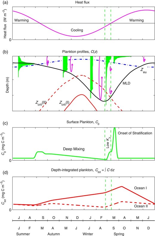
Schematic annual cycles for the temperate and subpolar oceans where deep winter mixing replenishes nutrients, (a) air-sea heat flux; (b) phytoplankton concentration profiles (filled profiles), along with the ML depth (MLD, solid line), the depth of the photic zone (Z_eu, dash-dotted line). Also shown are critical depths (Z_crit, dashed and continuous lines) for hypothetical Oceans I and II, where Ocean II is light-limited in winter, whereas Ocean I is not. The vertical scale of the mixing is indicated by overturn arrows; (c) surface plankton concentration, C₀; and (d) depth-integrated phytoplankton, C_tot, for the two hypothetical Oceans. Vertical dashed lines show the times of deepest ML and the cessation of vertical overturn. These times mark the transition from deep-mixing to low-turbulence to stratified regimes, respectively (see text). The x-axis shows northern and southern hemisphere months.

In autumn, heat fluxes become negative (i.e. out of the ocean), convective overturns starts and wind stress (not shown in Fig. 1) increases. As a result, the seasonal thermocline begins to deepen. This deepening mixes up the existing subsurface phytoplankton resulting in a small bloom in C₀. It may also entrain new nutrients into the ML, resulting in increased production and thus an increase in C_tot (e.g. Findlay, 2005).

The ML continues to deepen through autumn and winter, driven primarily by convective overturn. Observations (e.g. Backhaus et al., 2003) suggest that this convective overturn is generally strong enough to mix phytoplankton throughout the ML and the ocean enters what we term the ‘deep-mixing’ regime (Fig. 2). During this deep-mixing regime, phytoplankton and grazer concentrations in the ML will decrease because of dilution (e.g. Evans and Parslow, 1985), and C₀ will generally decrease, although in principle, if depth-integrated production is high enough, it can overcome the dilution so that C₀ can continue to increase.

Fig. 2.

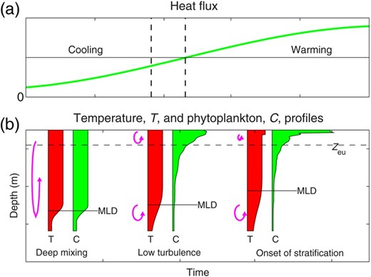
Schematic of the transition from deep-mixing to low-turbulence and then stratified regimes, (a) heat flux with dashed lines showing the times of deepest ML and the cessation of vertical overturn; and (b) profiles of temperature, T and phytoplankton, C (filled profiles). The vertical scale of the mixing is indicated by the overturn arrows, and the ML depth (MLD) is shown based on a density difference relative to surface values. During deep mixing in winter, both temperature and phytoplankton are well mixed to the MLD. In late winter or early spring, convective overturn becomes weak enough that it cannot maintain this deep mixing, and the ocean enters the low-turbulence regime, where the ML becomes remnant. In the low-turbulence regime phytoplankton are not well mixed vertically and can accumulate in the photic zone (Z_eu). When the heat flux becomes positive, shallow warm surface layers appear. This stratification can support a strong surface spring bloom. During the transition from deep mixing to stratified regimes, diapycnal mixing across the pycnocline, causes a MLD defined by a density difference criterion to rise. This can lead to a correlation between MLD ‘shoaling’ and bloom initiation.

The depth-integrated biomass, C_tot, can either increase or decrease during the deep-mixing regime, depending on whether depth-integrated production exceeds losses. During this deep-mixing regime, the Sverdrup assumptions are met (assuming nutrients are not limiting), and the CDH holds, so that depth-integrated accumulation will be positive if the ML is shallower than Z_crit.

We show two hypothetical Oceans in Fig. 1. Ocean I is where depth-integrated accumulation increases throughout winter, whereas in Ocean II, the phytoplankton within the water column become light-limited. Ocean II is the classic light-limited ocean that is the necessary winter precursor in the SMLH.

Towards the end of winter, convective overturn slows down and eventually becomes so weak that it cannot maintain a deep ML, and the ocean enters what we term the ‘low-turbulence’ regime (Fig. 1). During the low-turbulence regime, the ML becomes remnant, and vertical mixing becomes less than the critical value, so that as described by the CTH, phytoplankton concentrations increase in the photic zone, but decrease below it (Fig. 3). Irrespective of whether the Ocean is type I or II, surface phytoplankton concentration, C₀, will increase.

Fig. 3.

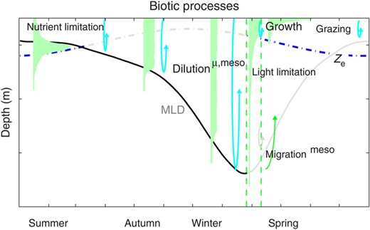
Schematic of annual cycles in biotic processes. Physical processes are shown as from Fig. 1, with those directly affecting production at any given time emphasized. In autumn and winter, when the ML depth (MLD) is deepening, vertical mixing is likely to be high enough that phytoplankton, micro- and mesozooplankton are well mixed in the ML, and dilution of phytoplankton may lead to lower grazing rates. Once the water column enters the low-turbulence regime, phytoplankton may become stratified in the ML. They are then light-limited below the photic zone but can bloom within it. When surface heat fluxes become positive into the ocean, near-surface stratification can support a bloom in surface phytoplankton. Ontogenetic migration of mesozooplankton into the upper water column in early spring may be timed to take advantage of this seasonal growth. From late spring, grazing and nutrient depletion near the surface, and light limitation below the photic zone then lead to summer conditions.

The transition from deep-mixing to low-turbulence regimes can occur before the heat flux becomes positive, but occurs about the time of the deepest ML. After this time (deepest ML), the MLD appears to shoal because of diapycnal mixing across the pycnocline. This diapycnal mixing weakens the density gradient over the pycnocline, so that MLs defined by a density difference relative to surface rise. Figure 2 illustrates this in terms of temperature: as the thermocline gradients weaken, the level that is 0.5°C cooler than the surface temperature rises. This shoaling can lead to an apparent correlation between MLD shoaling and bloom initiation.

In spring, heat fluxes eventually become positive and the ocean begins to stratify. As described by the OSH, this initially shallow but weak stratification can support a strong spring bloom at the surface, and both C₀ and r₀ reach maximum values (Fig. 2). Depth-integrated biomass, C_tot, may also increase as a result of this bloom.

As spring progresses, the water column continues to stratify. Grazing and nutrient depletion near the surface, and light limitation below the photic zone then decrease phytoplankton biomass, so that eventually summer conditions return. There may be also a loss of phytoplankton due to direct and/or indirect sinking (e.g. Nodder et al., 2005).

It is worth noting that in Figs 1 and 3, we have drawn the MLD as a continuous line throughout the year, and this is likely to be how an MLD defined by a 0.125 kg m⁻³ density difference criterion behaves. However, once this ML becomes remnant, this level does not represent the level of vertical mixing.

SUMMARY AND DISCUSSION

We have described a phytoplankton annual cycle that is driven by the physical processes of light, heat flux, wind stress, vertical overturn and vertical mixing (Figs 1 and 2), with the biotic responses of photosynthesis, respiration and grazing controlling the actual production and consumption of phytoplankton (Fig. 3).

This model combines the CTH and OSH with an emphasis on the transition from a deep-mixed regime in winter to a stratified regime in spring via an intermediate regime of low turbulence (Fig. 2). Our perspective recognizes that phytoplankton are not always mixed throughout the so-called ML, and that it is important to distinguish blooms in surface phytoplankton from blooms in depth-integrated phytoplankton.

The test of any hypothesis is whether it is supported by observations, and we suggest that existing observations support our view. For example, our model predicts that surface phytoplankton, C₀, can show autumn and spring blooms, as often seen in both the North Atlantic and South Pacific Oceans (e.g. Findlay, 2005; Henson et al., 2009; Chiswell et al., 2013).

Our model predicts that the winter minimum in C₀ occurs about the time of deepest MLD, as seen by Boss and Behrenfeld (Boss and Behrenfeld, 2010, their Fig. 2). It also explains why C₀ starts to increase before the cessation of vertical overturn, but the maximum rate of growth in C₀ does not occur until after the crossover in heat flux (Taylor and Ferrari, 2011b, their Fig. 10; Chiswell et al., 2013).

Our predictions for depth-integrated phytoplankton, C_tot, are less prescriptive, allowing for either increasing or decreasing C_tot during winter. Whether C_tot increases or decreases during winter depends on the local deep-mixing (vertical overturn) rates, nutrients, light levels and other biotic processes (species composition, grazing, etc.). Behrenfeld (Behrenfeld, 2010) suggested that the subpolar North Atlantic behaves as Ocean I. However, profiling float data from off Newfoundland (Boss and Behrenfeld, 2010, their Fig. 2) show C_tot decreasing during deep mixing in 2004–2005, but increasing during deep mixing the following year. It thus seems that at any given location, the ocean can be type I or II in different years. Chiswell et al. (Chiswell et al., 2013) suggested there may be a latitude dependence with higher latitude oceans more likely to enter a phytoplankton light-limited phase in winter.

Our model is largely ‘bottom-up’ driven, where the timing of the annual cycle is controlled by the timing of the physical drivers, but ‘top-down’ processes (e.g. grazing) often control the magnitude of the phytoplankton response. For example, ontogenetic migration of mesozooplankton (Thorisson, 2006) is a strategy by which grazers may be well positioned to take advantage of the enhanced prey concentrations associated with the spring bloom, and tightly couple production and losses at that time.

To unambiguously determine what drives ocean primary production by fully resolving the temporal and spatial variability in the driving terms (⁠$\mu ,\rho ,g$⁠) from observations would be prohibitively expensive. However, focussed experiments can eliminate one or other hypothesis, using relatively cheap instrumentation such as Bio-Argo (i.e. Argo floats equipped with sensors such as fluorometers, and/or transmissometers). For example, Bio-Argo data from Xing et al. (Xing et al., 2014, their Fig. 5) show that none of chlorophyll, particle backscatter, nor particle beam attenuation, are well mixed throughout the ML during the spring, suggesting the SMLH can be immediately discarded for the subpolar North Atlantic.

Reanalyses of existing satellite data, similarly, may help exclude one or other hypothesis. The timing of surface blooms relative to the driving terms has been used in support of these hypotheses (e.g. Obata et al., 1996; Ferreira et al., 2015). However, since correlation can be coincidental, rather than causal, reanalyses of such data should be aimed at excluding hypotheses.

It is worth commenting on the validity of the existing hypotheses. Chiswell (Chiswell, 2011) suggested the SMLH should be dismissed for the South Pacific because phytoplankton are not well mixed to the pycnocline in spring. He also suggested that the CDH is valid in winter, whether this is true globally has yet to be tested.

The main appeal of the DRH is that it provides a biological mechanism to explain any increases in C_tot during deep mixing, although it simplifies the complex ways in which dilution impacts the grazing efficiency (e.g. Fenchel, 1980). The DRH does not provide an explanation for the timing of blooms in surface phytoplankton.

The CTH and OSH differ largely in the interpretation of what constitutes a bloom (reflecting the fact that different metrics of bloom initiation favor different hypotheses). The CTH considers the bloom to start when surface values start to increase (i.e. when r₀ becomes positive), whereas the OSH considers the bloom start when r₀ reaches near maximum values. Our interpretation reconciles these differences by suggesting that surface phytoplankton concentration starts to increase at the transition from deep-mixing to low-turbulence regions, but that maximum accumulation rates occur only after the formation of surface stratification, when phytoplankton become trapped near the surface.

The conceptual model presented here is based on observations from the North Atlantic and South Pacific Oceans. We suggest the model is valid for oceans that have a phytoplankton cycle driven by nutrient replenishment during deep winter mixing. It is not valid for regions where the annual cycle is controlled by nutrient availability, e.g. in the tropics.

The model is one-dimensional in the vertical, and neglects horizontal processes that can impact water column stratification such as eddy-driven slumping of the density field (e.g. Taylor and Ferrari, 2011a; Mahadevan et al., 2012). These horizontal processes will impact the mechanisms leading to the deep-mixing, low-turbulence and stratified regimes. For example, eddy-driven slumping of the density field can lead to stratification before the cessation of convective overturn. However, we suggest that three regimes provide useful classification for the physical and biotic processes driving production, and the broad sequence of events is likely to be valid even in a three-dimensional world.

Finally, we return to Sverdrup's (Sverdrup, 1953) legacy. It is worth noting that Sverdrup never intended that the ML be taken to shoal in the spring. In fact he states ‘as the season advances, there develops a shallow mixed layer. . . . This development may be caused by spring heating…’. A developing surface ML from heating is not the same as a shoaling ML. We suspect that the SMLH stems from misinterpretation of Sverdrup's statement ‘On 4 April the depth of the mixed layer was for the first time smaller than the critical depth, and on the following day an appreciable phytoplankton population was recorded’. Examination of his Fig. 2 shows that the cause of the phytoplankton increase in May 1949 was due to Z_crit deepening with time, rather than a shoaling ML.

In our opinion, Sverdrup's (Sverdrup, 1953) legacy is that he formalized the concept of a critical depth, and showed why this depth is several times deeper than the photic zone, thus explaining why net primary production can be positive in water columns that might otherwise be considered light limited. This concept is valid and can be used successfully to test primary production in winter, but not in spring.

FUNDING

S.M.C. was funded by a grant from the New Zealand Government to the National Institute of Water and Atmospheric Research. P.H.R.C. acknowledges support from Conselho Nacional de Desenvolvimento Científico e Tecnológico (CNPq) – Bolsa de Produtividade em Pesquisa (Process: 307385/2013-2). P.W.B. was supported by University of Tasmania.

ACKNOWLEDGEMENTS

We thank four reviewers for their careful and conscientious reviews.

Author notes

Corresponding editor: Roger Harris