Dynamic Inconsistency in Food Choice: Experimental Evidence from Two Food Deserts

Abstract

We conduct field experiments to investigate dynamic inconsistency and commitment demand in food choice. In two home grocery delivery programs, we document substantial dynamic inconsistency between advance and immediate choices. When given the option to commit to their advance choices, around half of subjects take it up. Commitment demand is negatively correlated with dynamic inconsistency, suggesting those with larger self-control problems are less likely to be aware thereof. We evaluate the welfare consequences of dynamic inconsistency and commitment policies with utility measures based on advance, immediate, and unambiguous choices. Simply offering commitment has limited welfare (and behavioural) consequences under all measures.

1. Introduction

Models incorporating temptation impulses and self-control are among the most prominent in behavioural economics (Strotz, 1955; Thaler and Shefrin, 1981; Laibson, 1997; O’Donoghue and Rabin, 1999; Gul and Pesendorfer, 2001; Fudenberg and Levine, 2006). The dynamic inconsistencies predicted by these models provide a reason for the observed difficulty of people to save more for the future, exercise more, eat healthier, and quit smoking. Based on the insights generated by these models, prescriptions such as offering commitment devices have grown prominent in policy circles.

In this article, we address a core question in the literature on policies for self-control. What is the relationship between dynamically inconsistent behaviour and beliefs thereof? The value of commitment policies for altering outcomes depends principally on this relationship. If individuals with the greatest self-control problems are the most likely to be unaware of them, take-up would be concentrated among those for whom the policy has the least effect. In such cases, a policy offering commitment should deliver limited effects on behaviour. While the apparent tepid demand for commitment outside of controlled experimental settings is consistent with broad unawareness, there is a notable lack of evidence on the central correlation between behaviour and beliefs necessary for policy evaluation.¹

Several experimental studies find weak positive correlations between hallmarks of dynamic inconsistency and take-up of products with commitment features (Ashraf et al., 2006; Augenblick et al., 2015; Kaur et al., 2015). This indicates at least a weakly positive correlation between self-control problems and awareness. Augenblick and Rabin (2018) confirm this weak positive correlation by eliciting both behaviour and beliefs in a laboratory experiment on effort choices, while John (2018) shows zero correlation between self-control issues measured over money and a general survey measure of awareness.² Little is known about the relationship between behaviour and beliefs in real-world settings. Given that the impact of commitment policies depends on this real-world relationship, data from field settings have the potential to provide substantial value.

We combine an elicitation of dynamic inconsistency and take-up of commitment devices in a field setting to examine the relationship between behaviour and beliefs, and to provide an assessment of the effects of commitment policy. Our field experiments are conducted in a natural setting, and individuals are not told that they are in an experiment, which mimics naturally occurring markets. Further, our experiments test dynamic inconsistency over consumption using longitudinal decisions with limited scope for arbitrage, which aligns tightly with theoretical models. Finally, we collect within-subject data on dynamic inconsistency and commitment over time, which allows us to investigate stability of these measures.

Our setting is a food delivery service for low-income participants in two cities: Chicago, Illinois and Los Angeles, California. Three hundred eighty-nine subjects completed a 3–4-week food delivery program. Subjects were given a budget and asked to construct a bundle from a list of 20 foods for home delivery 1 week later. On the day of delivery, the delivery person brought the pre-ordered bundle and also surprised subjects with additional foods available for exchange. Subjects were given the opportunity to make up to four exchanges. Every bundle that could be constructed with immediate exchanges (on the day of the delivery) is one that was available at the time of advance choice (1 week earlier). As such, dynamic inconsistencies are identified as violations of revealed preference between advance and immediate choices.

In the second and third weeks of the study, subjects again made advance choices. However, before the delivery, they were asked if they would like the option to make exchanges at delivery again, or whether they would like to stick to their pre-ordered choices. Commitment demand is identified as choosing to restrict oneself to the advance bundle. The correlation between dynamic inconsistency (in the first week) and subsequent commitment demand provides data on the relationship between self-control problems and awareness thereof that can be used to evaluate commitment policies.

We find that when commitment is not available, 46% of subjects exhibit dynamic inconsistencies, exchanging at least one item from their advance bundle. Regularities exist in the nature of these inconsistencies. Immediate bundles contain significantly fewer fruits and vegetables and more calories (primarily from fat) than advance bundles. When commitment is available, 53% of subjects take it up, preferring to restrict themselves to their advance bundle. Importantly, subjects who were previously dynamically inconsistent are less likely to demand commitment (44%) than subjects who were previously dynamically consistent (60%). This negative correlation suggests that those with the largest self-control problems may lack sufficient awareness to demand commitment.

A structural estimation exercise that formulates utilities in terms of food characteristics indicates the value of fruits and vegetables is significantly lower in immediate versus advance choice. The structural estimates are built using standard random utility methods and allow for tests that inconsistencies would arise by chance under dynamically consistent preferences. Tests of consistent preferences are rejected for the aggregate data and for inconsistent subjects at all conventional levels. Utility estimates from when commitment is not available show that subjects who ultimately commit have substantially smaller differences between advance and immediate preferences than those who ultimately do not commit. These structural conclusions corroborate the reduced-form findings discussed above and our structural predictions closely match behaviour in-sample.

As noted above, if individuals with the largest self-control problems are the least aware thereof, policies offering commitment may have limited impacts on behaviour. We demonstrate this empirically in our setting both longitudinally and using a sub-sample of subjects who are offered commitment at random. Offering commitment has statistically no effect on the characteristics of bundles ultimately consumed.

Potential commitment policies should not be evaluated solely on their impact on behaviour. Support for a given policy should depend on its welfare consequences. Here, as well, the literature on dynamic inconsistency is lacking research evaluating the welfare outcomes of commitment policies. One core challenge in conducting such an exercise is the choice of welfare criterion. Ambiguity in welfare evaluations may exist in the context of self-control problems given potential inconsistency between “long-run” preferences measured absent temptation and “short-run” preferences measured under temptation. A practice has emerged that bases welfare calculations on long-run preferences under the positive justification that short-run preference deviations represent mistakes (Herrnstein et al., 1993; Gruber and Kőszegi, 2001; O’Donoghue and Rabin, 2006). Nonetheless, it must be recognized that this is simply tradition, and it may be more than an intellectual curiosity to examine the effect of policies on “short-run” preferences. One clear reason to be interested in “short-run” welfare measures is that the choice to renege on a commitment that can be unwound will be related to such quantities.

The “short-run” and “long-run” measures are not the only values researchers may wish to consider. Additionally, a burgeoning literature in behavioural welfare economics advocates for basing welfare analysis on unambiguous choices—i.e. choices that are consistent across the long- and short-run. Bernheim and Rangel (2007, 2009) pioneered this approach and provided a theoretical evaluation for the example of dynamic inconsistency. To our knowledge, there exists no empirical evaluation of the welfare consequences of dynamic inconsistency and commitment policies recognizing potential disagreement across welfare criteria.

To understand the welfare consequences of commitment policies, we evaluate welfare under three measures: the estimated advance utility and immediate utility noted above; and an unambiguous utility estimated in a similar fashion using only foods that were never exchanged, being either chosen or unchosen in both advance and immediate choice.³ For all three utility estimates, all foods have projected values. For example, we can use the utility weights for food attributes estimated under advance preferences to project the values of foods chosen in immediate bundles, constructing the value of the immediate bundle under advance preferences. Contrasting this with the projected value of the advance bundle, itself, generates a measure of the welfare consequences of inconsistency under advance utility. Because each food has a value informed by the body of other food choices, it may be that inconsistencies that replace a low projected value food with a high projected value food lead to an estimated benefit to inconsistency under the advance utility measure or an estimated cost to inconsistency under the immediate utility measure.⁴

The advance and immediate utility measures yield intuitive results at the individual level for the welfare consequences of dynamic inconsistency and offered commitment. For dynamically inconsistent individuals, the median subject’s advance utility predicts welfare costs to inconsistency on the order of around 5% of utility, while immediate utility predicts welfare benefits to flexibility of roughly equal size. Where this disagreement exists, the conflict between advance and immediate welfare measures may be helpfully arbitrated by the unambiguous utility measure. Fifty percent of inconsistent subjects have unambiguous welfare reductions due to inconsistency. The advance and immediate measures similarly disagree on the value of commitment, with advance utility generally predicting benefits and immediate utility predicting costs thereto. Nonetheless, the overwhelming majority of committing subjects are dynamically consistent and so have no welfare consequences therefrom. Indeed, overall roughly 80% of subjects’ welfare is unaffected by the commitment offer, regardless of the utility measure. Following the limited effects on behaviour, our policy offering commitment likely had similarly limited effects on welfare.

In addition to examining the policy of offering commitment, we also analyse the behavioural and welfare consequences of two further policies. The first is a policy that mandates advance choice. This policy affects a greater percentage of subjects than simply offering commitment—around 45%—and leads to perceptibly larger behavioural effects. However, mandated advance choice does generate a substantial fraction of individuals who are made worse off: from around 15% under the advance measure to around 30% under the immediate measure. The second policy that we analyse is a tailored policy that mandates advance choice only for people who, by our estimates, exhibit unambiguous costs to inconsistency. Interestingly, this policy affects around the same percentage of subjects as offering commitment—around 20%—but has dramatically fewer worse off individuals under all estimated preferences, from 0.2% under the advance measure to 7% under the immediate measure.⁵ The surprisingly unanimous benefits to the tailored mandate are driven by limited correlation between the advance and immediate utility measures, but strong correlation between the unambiguous utility measure and the other two utility measures. Given this consensus, there may be some value in considering the implementation of such a policy in future applications.

Our two core findings: dynamic inconsistency reflecting changing preferences between advance and immediate choices; and a negative correlation between dynamic inconsistency and demand for commitment are observed at both study sites. The original version of this article featured only data from Chicago. Los Angeles was added as a full-scale replication and extension of the previously documented findings. Replicating the findings—in particular, the demonstration in field data that those with the most substantial self-control problems may be the least aware thereof—helps to assure the results are not obtained simply by chance.

This article provides contributions along three principal avenues. First, our data on commitment demand provide evidence on a central assumption around which policy prescriptions for behavioural consumers are built. We show demand for commitment but find that agents who demand commitment have systematically smaller self-control problems than those who do not. Much of the previous literature on self-control has relied on tests of diminishing patience over monetary rewards rather than consumption, and has used decisions made at a single point in time rather than longitudinally (Sayman and Onculer, 2009; Halevy, 2015; Sprenger, 2015, provide discussion).⁶ With the exception of Read and Van Leeuwen (1998), who studied snack choice among employees but did not study commitment, participants in these studies knew they were part of an experiment, which could affect their decisions. We study subjects in their natural setting, which could explain the difference in our results relative to the weakly positive correlation between self-control and awareness implied by prior research.

Second, our experimental populations sit in the cross-hairs of the food policy debate. Our neighbourhoods are considered “food deserts,” implying a high rate of poverty and limited access to fruits and vegetables.⁷ Obesity and related diseases are at an all-time high in the U.S., are largely driven by poor food choice, and disproportionately affect low-income communities.⁸ Americans consume fewer than the recommended servings of fruits and vegetables, and more than the recommended servings of high-calorie, low-nutrient foods. Food assistance programs such as the Supplemental Nutrition Assistance Program (SNAP) are one tool for improving healthfulness of food choice in low-income communities. A policy change is now being piloted that would allow retailers to accept SNAP dollars for pre-ordered food.⁹ Our results add to an understanding of the impact of this policy change on behaviour and welfare. Indeed, our findings indicate that this policy will have limited behavioural and welfare effects; and suggest alternatives for structuring more beneficial policies.

Third, our exercise provides a demonstration of the value of combining structural methods and behavioural welfare analysis. Behavioural welfare measures require that researchers do not arbitrarily honour a given preference ranking without a clear reason to do so. In dynamically inconsistent choice, this delivers a natural intuition that virtually nothing concrete can be said with regards to welfare. We demonstrate that this is not necessarily the case. In our structural setting, the body of food choices are informative of how decision-makers value food characteristics. Through the lens of the model, we construct and compare welfare measures that deliver clear welfare implications. And we join a small list of empirical studies that investigate the welfare consequences of behavioural phenomena (Chetty et al., 2009; Allcott et al., 2014; Allcott and Taubinsky, 2015; Rees-Jones and Taubinsky, 2016; Taubinsky and Rees-Jones, 2018). We join an even smaller list of empirical projects that recognize the corresponding ambiguity in welfare estimates that may arise in behavioural settings (for one recent example, see Bernheim et al., 2015).

In what follows, Section 2 provides an overview of the experimental design and describes the structural analysis, Section 3 describes our results and Section 4 concludes.

2. Empirical Design

2.1. Experimental setup

We conducted two field experiments with a total of 389 subjects at grocery stores in Chicago, Illinois and Los Angeles, California.¹⁰ The first experiment was implemented with 218 subjects in 2014 at Louis’ Groceries, a small-format neighbourhood grocery store in the low-income community of Greater Grand Crossing in Chicago. The second experiment was implemented with 171 subjects in 2016–7 at Northgate Gonzalez Market, a large supermarket in low-income South-Central Los Angeles.¹¹

The grocery stores carried out a promotion inviting customers to sign up for a free home food delivery program. Recruitment for both experiments was conducted on a rolling basis. Two research assistants worked at each grocery store to conduct the experiment and deliver the foods. Subjects for the study were recruited at a table set up at the store. We assured that foods were fresh and produce was not bruised at the time of delivery by working with the grocery stores and preparing deliveries as close to the delivery time as possible. In keeping with the natural field experiment methodology, subjects were not told that they were in an experiment.¹² In the Los Angeles study, to increase naturalism, research assistants partnered with a store associate to deliver items in the Northgate store delivery van. Thus, we were able to observe subjects in their natural environment as they made a series of food allocation decisions.

A total of 20 different foods were used in each experiment. Figure 1 displays the promotion sheet of foods used. Foods were selected in consultation with store managers to determine which foods would be appealing to customers at each site. In each study, 10 of the foods were fruits or vegetables while the other 10 were sweets or salty snacks. Foods varied substantially in their caloric and nutritional content. Supplementary Table A1 provides nutritional information for the foods included in each study.

Figure 1

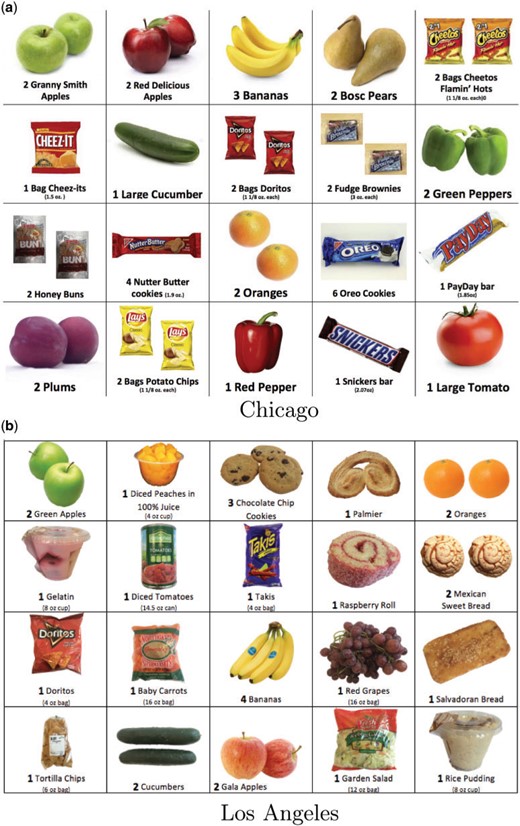
Study foods

Upon signing up for the program, subjects were asked whether they had eaten each of the 20 foods before and then rated those they had eaten on a Likert scale from 1 (least preferred) to 7 (most preferred). The use of Likert scales to rate foods has been promoted in the nutrition literature as a means of assessing dietary preferences (Geiselman et al., 1998).¹³ Subjects were generally aware of and had eaten all 20 of the foods. On average, subjects rated 18.6 of 20 foods and the average food rating was 5.58 out of 7.¹⁴

In return for participating in the program—including selecting foods, receiving the weekly deliveries, and completing surveys—subjects received a participation payment. This payment was a

$\$$

20 cash voucher in the Chicago study and a

$\$$

25 Northgate store gift card in the Los Angeles study.

2.2. Experimental timeline

The experimental timeline is presented in Table 1. The Chicago study offered a 2-week food delivery program while the Los Angeles study offered a 3-week food delivery program. In Week 1, each subject decided on foods for delivery in Week 2. Upon receiving the delivery in Week 2, each subject was surprised with the option to make immediate exchanges. In Week 2, each subject also decided on foods for the second delivery in Week 3. All Chicago subjects subsequently made a commitment choice, deciding whether to have the option to make exchanges (i.e. not commit) or to stick to their pre-ordered choices (i.e. commit) for the second delivery. To investigate the stability of inconsistency and commitment demand, we randomly assigned half of the subjects in Los Angeles to receive commitment offers for both the second and third delivery. We assigned the other half to make a second surprise exchange and offered this group commitment only for the third delivery.

Table 1

Summary of experiment

Week 1	Week 2	Week 3	Week 4 (L.A. only)
Pick Delivery 1 items	Get Delivery 1	Get Delivery 2	Get Delivery 3
	Decide about changes to Delivery 1	If no commitment: decide about changes to Delivery 2	If no commitment: decide about changes to Delivery 3
	Pick Delivery 2 items	Pick Delivery 3 items (L.A. only)
Pre-survey Food Ratings	Commitment choice for Delivery 2 (Chicago & half of L.A. subjects)	Commitment choice for Delivery 3 (L.A.only)	Post-survey (Week 3 in Chicago)

2.2.1. Week 1, advance choice

In Week 1, subjects received an order sheet and brochure listing available foods and decided on foods for their first delivery. All foods were also available at the store, and the fresh foods were visible to the subjects as they made their decisions. To simplify the selection process, each food was valued at

$\$$

1, with cheaper foods bundled into several for

$\$$

1 (e.g. 2 green apples together cost

$\$$

1). All foods were priced as closely as possible to their respective market price. Subjects were asked to create a “basket” of foods valued at

$\$$

10 in total, by choosing from any of the 20 foods, including selecting the same food more than once. Subjects also selected their preferred dates and times of delivery.

Subjects were informed that they would need to be home during their delivery, and would need to show a picture ID to receive their basket. Delivery was scheduled as close to 7 days after sign up as possible, taking into account the constraints faced by the research assistants (i.e. a maximum number of deliveries can be made in any day) and the availability of the subject. Subjects were required to give a current phone number and address to facilitate delivery. All subjects received a phone call to confirm enrolment upon sign up, which also allowed us to validate their phone number.

2.2.2. Week 2, immediate choice

A few days before scheduled delivery in Week 2, we initiated a reminder call to ensure that subjects would be home at the pre-arranged time and then proceeded with delivery. Upon delivery, subjects were surprised with the opportunity to make up to 4 exchanges. In Chicago, we brought a customized box of 4 foods selected from the 20 that were available previously, whereby we tried to select foods that the subject liked. This box contained their highest rated fruit or vegetable, their highest rated fruit or vegetable not included in their original bundle, their highest rated sweet or salty snack and their highest rated sweet or salty snack not included in their original bundle. In Los Angeles, we brought a box with one of each of the 20 foods that were available previously, and subjects could make exchanges with any of these foods. As before, cheaper foods were bundled into several for

$\$$

1. Subjects were not told in advance that they would have this opportunity to exchange. The opportunity to exchange was described by a research assistant serving as a delivery person and was fully scripted as:

Hello, I am here with your basket. Please take a look [Bring open basket, allow person to look through]. We also have some extra items available. If you like, you can exchange any one item in your basket for one of these items [ show extra items on tray ]. I brought 4 additional items, so you can make up to 4 exchanges. Do you want to make any exchange? [Great thanks, let me note that on your order sheet.]¹⁵

After making any exchanges, subjects used a new order sheet to make a decision about the contents of their second delivery, scheduled for Week 3.

2.2.3. Weeks 2–3, commitment choice

We elicited demand for commitment by asking subjects whether they would like to have the option to make exchanges during the Week 3 delivery, or whether they would like to stick to their pre-ordered choices. We asked this of all subjects in Chicago and half of subjects in Los Angeles. The question was again fully scripted in both study locations. In Chicago, the script was:

Last time, we brought some extra items for you so you could exchange if you changed your mind from your previous choices. This time, we can also bring extra items, but I wanted to check if you’d like that or not. It is up to you: would you like me to bring extra items this time, or not?

In Los Angeles, the script was:

For this week’s delivery, you had the option to change your mind by exchanging items in your basket. This time, you can choose whether you want the option to make exchanges, or whether you want to stick to your pre-ordered choices. It is no trouble for us either way, it is entirely up to you. Do you want to have the option to make exchanges, or do you want to stick to your pre-ordered choices?

In Chicago, the commitment question was asked via phone during the reminder call before the next delivery. In Los Angeles, the commitment question was asked in person immediately after the order for the next delivery was placed. If a subject answered that they wanted to have the option to make exchanges, additional items were presented at the next delivery as before. If a subject answered that they would like to stick to their pre-ordered choices, the box of additional items was not brought along with the delivery.

2.2.4. Weeks 3–4, final delivery and commitment choice

The subjects in Los Angeles not assigned to the commitment treatment were offered the opportunity to make exchanges in Week 3. The subjects in Los Angeles assigned to the commitment treatment only had the option to make exchanges if they previously chose not to commit. After delivery in Week 3, all Los Angeles subjects used a new order sheet to make a decision about the contents of their third delivery, scheduled for Week 4. After completing this order sheet, all subjects were asked the commitment question applied to their Week 4 delivery. At the final delivery (Week 3 for Chicago and Week 4 for Los Angeles), subjects completed a survey and received compensation for participating.

2.3. Design considerations

Our Chicago and Los Angeles studies follow similar procedures. The Los Angeles study was constructed as a replication and extension and so allowed us to address potential concerns with respect to identifying dynamically inconsistent preferences and commitment demand. We are indebted to thoughtful comments from colleagues that helped guide these design alterations.

First, dynamic inconsistencies are identified from exchanges between advance and immediate food choice. An intuitive direction of inconsistency is exchanging objects such as fruits and vegetables for sweets and salty snacks. An interpretation that attributed such inconsistencies to changing preferences could be challenged by several concerns in the Chicago design. First, in the Chicago study, all fruit and vegetable items were perishable while no sweets and salty snacks were perishable. If perishable items wound up being damaged, spoiled, or less attractive than expected upon delivery, exchange could be driven by such negative surprises rather than by inconsistent preferences. Naturally, the potential for such damage should be forecasted by subjects and so influence advance decisions taken without knowledge of the opportunity to reallocate. Under correct forecasts, immediate foods should be as damaged as expected, limiting systematic inconsistencies. Nonetheless, in reaction to this potential critique, our Los Angeles study was designed with primarily perishable items, only 2 non-perishable fruit and vegetable items (diced peach cup and canned diced tomatoes) and 2 non-perishable snack items (Doritos and Takis Chips). Additionally, 2 fruits and vegetables came in factory packaging (baby carrots and salad) while most snack items came from the bakery department without factory packaging (e.g. Salvadoran bread).

Second, in our Chicago study, we brought only 4 additional items selected based on subjects’ rating data. Any lack of dynamic inconsistency could be driven by our inability to match subjects with tempting items for exchange. Though this suggests any exchanges would speak to a lower bound on inconsistent preferences, in the Los Angeles study we improved on this design by making all 20 items available for exchange. To keep the designs as similar as possible, however, we retained the design element of allowing only up to 4 exchanges. In practice, this restriction rarely binds, with only 1 of 389 subjects making 4 exchanges at their first delivery.

Third, our Chicago subjects only made one exchange decision prior to being offered commitment. It may be that any observed dynamic inconsistency is ephemeral, a product of shocks or changing circumstances. These random shocks should not deliver a systematic direction for inconsistency. Nevertheless, having more data at the subject level as we do in the Los Angeles study allows us to further rule out that the inconsistencies are due to random shocks.

Fourth, the phrasing of our commitment offer in Chicago may have had the unintended effects of making commitment appear socially desirable and/or may have failed to emphasize that commitment induces a restriction to advance choice. Subjects who did not want to trouble the delivery person may have opted to commit to save him or her work. Subjects opting out of the exchange opportunity may not have realized that this was equivalent to a choice to commit to the advance bundle. For these reasons, the Los Angeles study script highlights that neither choice is more costly for the delivery person, and that the decision to commit is equivalent to sticking with advance choice. Ultimately, there are many ways in which a commitment offer could be presented to subjects, possibly with unintended information transmission or demand effects. Our objective was to control these with an explicit script for behaviour (informed in our Los Angeles site by referee feedback). Nonetheless, there remain plausible demand effects in both study sites which could influence the level of commitment take-up. Importantly, our exercise focuses on the correlation between take-up and dynamic inconsistency. Hence, any rationalization of our data based on demand effects must also feature differential demand effects across levels of prior dynamic inconsistency.

In both of our studies, we observe choices but not consumption of food items. One may worry that subjects’ choices do not represent their true preferences, but rather reflect their external opportunities to trade food items. For example, a subject who can trade tomatoes for chips more advantageously outside of the experiment may choose a bundle consisting only of tomatoes, conduct appropriate trades and generate for herself an opportunity set which dominates that provided by the researchers. Such arbitrage would imply that subject choices are not informative of preferences at all, but rather only of external constraints and the researchers’ mis-pricing of items.¹⁶ Several aspects of the experimental environment minimize the possibility of arbitrage. The prices in the stores are similar to those faced in the experiments. Hence, external exchanges are unlikely to be advantageous. Additionally, our stores are in “food deserts,” and many study foods—e.g. fresh fruits and vegetables and bakery goods—are difficult to obtain elsewhere. Conducting exchanges with others in the neighbourhood is also practically difficult given the cost of identifying interested parties and the perishability of some foods. Importantly, even if arbitrage opportunities exist, one would not expect them to change dramatically over a single week in our studies. Hence, if choice is driven by arbitrage strategies, dynamic inconsistencies should be rare. The data themselves can provide some indication of arbitrage strategies by examining the prevalence of completely concentrated bundles, consisting of only a single food. Such bundle concentration is never observed, with the median (mean) [25th, 75th percentile] advance first week bundle having 10 (9.3) [9, 10] unique items. Though subjects could choose more than one of the same item, 255 or 389 (66%) do not do so, and 318 of 389 (82%) do so no more than once in their advance bundles in the first week. Along with an absence of arbitrage, this may indicate that food-specific marginal utility diminishes quite quickly.¹⁷ Interestingly, we also rarely see a more limited version of concentration: subjects choosing exclusively fruits and vegetables or exclusively sweets and salty snacks. Only 14 of 389 (4%) advance bundles in the first week are concentrated this way.

An additional concern posed by not observing food consumption is that if foods are not consumed immediately, temptation may be limited. In our Los Angeles study, we measure the speed with which foods are consumed by including questions about consumption in our post-experiment survey. Subjects were asked, for the foods they ordered in their Week 3 delivery, how quickly they ate the foods—within 1–3 days, 4–7 days or in more than 7 days. Most foods were consumed within 1–3 days, ranging from 79% (for canned tomatoes) to 88% (for Mexican sweet bread). Importantly, the fruits and vegetables and perishable foods are eaten within 1–3 days as frequently as sweets and salty snacks and unperishable foods.¹⁸ This suggests that most foods are indeed being consumed rapidly, within the time frames thought to be relevant for temptation. That subjects do not apparently store more long-lasting foods helps to alleviate the perishability issue discussed previously.

Finally, commitment demand may be an imperfect proxy for awareness about self-control problems. An alternative approach is to elicit beliefs about future behaviour, as in Augenblick and Rabin (2018). We did not elicit beliefs for two reasons. First, we wanted to maintain the naturalism of the study. Second, using incentives to elicit beliefs (to make the beliefs incentive compatible) is also a form of providing a commitment device because deviating from predicted behaviour in immediate choice is costly (see Augenblick and Rabin, 2018, for discussion). Further, Augenblick and Rabin (2018) find that participants may seek to match their behaviour to earlier predictions, suggesting that predictions may affect future behaviour rather than serving purely as an exogenous measure of self-awareness.¹⁹

2.4. Structural analysis, dynamic inconsistency and welfare

Subjects in our experiments choose a bundle of 10 foods from a set of 20 potential options. From such data, reduced form and structural analysis of dynamic inconsistency in food choice can be conducted. The structural method we propose follows standard random utility techniques, establishing the value of a given item as being derived from a set of characteristics. This allows for simple tests of dynamically inconsistent preference, recognizing the existence of random shocks. The estimated utilities lend themselves naturally to evaluation of commitment policies under different welfare criteria.

Following methodology from Beggs et al. (1981), we define each food as a collection of underlying attributes and analyse subject choices using rank order discrete choice methods.²⁰ Let the utility of each food, |$j \in \lbrace 1, ..., J \rbrace$|⁠, be written as a linear combination of attributes,

$$\begin{eqnarray*} V_j = {\bf x}_j \beta + \epsilon_{j} & j = 1,..., J, \end{eqnarray*}$$

where |${\bf x}_j$| represents a vector of food characteristics and |$\epsilon_j$| represents a random utility shock drawn iid from a Type-1 extreme value distribution. The probability that a given food, |$j$| is preferred to alternatives |$1, ...,J-K-1$| is

$$\begin{equation*} F_j[x_1, ..., x_{J-K-1}, x_j; \beta] = {{\rm{exp}}({\bf x}_j \beta) \over {\rm{exp}}({\bf x}_j \beta) + \sum_{i=1}^{J-K-1} {\rm{exp}}({\bf x}_i\beta) }. \end{equation*}$$

Consider a subject who includes |$K$| unique food items in their bundle. Order the foods as |$ r \equiv \lbrace 1,..., J-K-1, J-K, J-K+1, ... J \rbrace $|⁠, with the final K foods being the excluded items. The probability of observing such an ordering is thus

$$\begin{equation*} Prob(r, {\bf x}; \beta) = \prod_{j=J-K}^J F_j[x_1, ..., x_{J-K-1}, x_j; \beta],\end{equation*}$$

where |${\bf x} \equiv \lbrace {\bf x}_1, ..., {\bf x}_J\rbrace $| is the matrix of attributes corresponding to the provided order. Indexing individuals by |$i = 1, ..., N$|⁠, one constructs the log-likelihood of seeing a given N rankings as

$$\begin{equation}\label{eq:loglikelihood} L(\beta) = \sum_{i=1}^N \log({\rm{Prob}}(r_i, {\bf x}_i; \beta)).\end{equation}$$

(2.1)

This structure assumes that any included item is preferred to all excluded items. Within the sets of included and excluded items, no explicit ranking exists. In the language of rank order logit models, the ranks within these sets are “tied” as all permutations of rankings within these sets would be consistent with observed behaviour. Standard methodology exists for incorporating the probability of these ties into maximum likelihood estimates of the parameter of interest, |$\beta$|⁠. We augment the probability of equation (1) with Efron’s (1977) method for handling ties in rank order data, implemented in Stata.

2.4.1. Tests of dynamic inconsistency

Consider two rankings of foods: one from advance decisions and one from immediate decisions. Let |$ r_A$| and |$r_I$| represent the advance and immediate rankings, respectively. Maximum likelihood estimation of attribute weights, |$\beta_A$| and |$\beta_I$|⁠, based upon these rankings provide a means of comparing preferences across choice environments. Further, |$\beta_A$| and |$\beta_I$| can be estimated simultaneously and one can test the null hypothesis of dynamically consistent preferences, |$\beta_A= \beta_I$|⁠, using standard |$\chi^2$| tests. Such tests establish the probability that observed exchanges would occur by chance under the extreme value error structure without dynamically inconsistent preferences.

Two points related to our structural tests of dynamic consistency are worth noting. First, in both of our studies, subjects were only allowed to make up to 4 exchanges. This restriction limits the inconsistencies that can be observed between |$r_A$| and |$r_I$|⁠. Though in practice, only 1 of 389 subjects made all 4 exchanges at their first delivery, this design feature could in principle, work against finding differences between |$\beta_A$| and |$\beta_I$|⁠. Second, in our Chicago study, our design called for bringing only 4 additional items when making food deliveries. As such, |$r_I$| may be additionally restricted to be similar to |$r_A$| by our inability to provide subjects with sufficiently tempting alternatives, again working against finding differences between |$\beta_A$| and |$\beta_I$|⁠. Our Los Angeles design does not suffer from this potential issue, as all foods were available for exchange when subjects made immediate choices. These points suggest that findings of dynamic inconsistency and the corresponding changes in preferences estimated in our study may be lower bounds.

2.4.2. Welfare evaluation

Estimated utility weights, |$\beta_A$| and |$\beta_I$|⁠, speak to two different potential welfare criteria based on advance and immediate preferences, respectively. One can construct an estimate of the deterministic utility portion of any proposed bundle under advance preferences as

$$\begin{equation*} V_A({\bf q}) = \sum_{j=1}^J q_j {\bf x}_j \beta_A, \end{equation*}$$

where |${\bf q} = \lbrace q_1, ...,q_j, ... q_J\rbrace $| is the proposed bundle with quantity |$q_j$| of food |$j$|⁠.²¹ Similarly, one can construct the immediate utility,

$$\begin{equation*} V_I({\bf q}) = \sum_{j=1}^J q_j {\bf x}_j \beta_I.\end{equation*}$$

These two measures can be used to evaluate the welfare consequences of dynamic inconsistency and commitment policies. In order to evaluate the welfare consequences of dynamic inconsistency, we calculate the percentage change in utility between advance and immediate bundles, |${\bf q_A}$| and |${\bf q_I}$|⁠, under each utility measure. For example, under the advance measure, the welfare consequences of inconsistency are

$$\begin{equation*} V_A({\bf q_A}) - V_A({\bf q_I}) \over V_A({\bf q_A}). \end{equation*}$$

Bundle values such as |$V_A({\bf q_A})$| are linear in the food-specific values, |${\bf x}_j \beta_A$|⁠. As such, a similar measure could express the difference in utility in terms of a single good’s value—such as the highest value food—rather than normalized by utility. Because such a “best-food” equivalent would have, perhaps, a more natural interpretation and connection to more traditional welfare measures, we also provide these values in the Supplementary Appendix. Additionally, using an alternate estimation technique for utility in robustness Section 3.3.3, we provide traditional measures of equivalent variation (in terms of the total number of foods), and compare to the measures obtained here.

It is critical to note that because utility weights, |$\beta_A$| and |$\beta_I$|⁠, are estimated from the body of included and excluded foods in advance and immediate choice, an exchange could be made that increases total utility from the advance perspective or decreases total utility from the immediate perspective. As such, inconsistencies will not be viewed as uniformly negative from the advance perspective or uniformly positive from the immediate perspective. We view this as a critical feature of having considered bundle inclusion as driven by both deterministic features and food-specific shocks. Some advance inclusions may have been made in error and subsequent inconsistencies may indeed increase the total bundle value from the advance perspective. In Section 3.3.3, we consider the robustness of our results using an alternate estimation strategy, based on bundle composition rather than bundle inclusion (which does not have this feature) and find quite similar results.

To evaluate commitment policies that potentially restrict immediate choice, we can calculate the effects again based on the estimated utility values. For example, advance utility will predict benefits to committing to the advance bundle if

$$\begin{equation*} V_A({\bf q_A}) > V_A({\bf q_I}). \end{equation*}$$

As above, commitment could be estimated to have negative or positive value under both utility measures. That is, under a given welfare criterion, a policy can leave individuals both worse off and better off. We view this as a feature of our exercise, which understands choice as a product of deterministic food values and random shocks.

If disagreement in choice, and hence potential differences between |$\beta_A$| and |$\beta_I$| exist, welfare statements may be ambiguous. Welfare measures |$V_A(\cdot)$| and |$V_I(\cdot)$| may disagree on the value of policies. Where disagreement in choice exists across welfare relevant conditions, Bernheim and Rangel (2007, 2009) advocate for formulating welfare statements around an unambiguous choice relation that never contradicts choice. By examining only foods that were never exchanged, we can construct this unambiguous relation. Consider the ordering |$r_U \equiv \lbrace 1,..., J-E-K-1, J-E-K, J-E-K+1, ... J-E \rbrace $| with the final |$K$| foods being the chosen items and |$E$| being the number of items that were ever exchanged from advance to immediate choice conditions. The likelihood

$$\begin{equation*} {\rm Prob}(r_U, {\bf x}; \beta_U) = \prod_{j=J-K-E}^{J-E} F_j[x_1, ..., x_{J-K-1}, x_j; \beta_U]\end{equation*}$$

can be used to estimate unambiguous utility values |$\beta_U$|⁠, ignoring any exchanged items. If no items are ever exchanged, the rankings are identical and |$\beta_U = \beta_A = \beta_I$|⁠. If exchanges are made, |$\beta_U$| can differ from both |$\beta_A$| and |$\beta_I$|⁠. One can evaluate the deterministic portion for unambiguous utility of a proposed bundle, |${\bf q}$|⁠,

$$\begin{equation*} V_U({\bf q}) = \sum_{j=1}^J q_j {\bf x}_j \beta_U,\end{equation*}$$

and construct corresponding calculations for the welfare effects of proposed policies.

Our treatment of unambiguous choices differs in one critical way from the Bernheim and Rangel (2007, 2009) approach. The Bernheim and Rangel (2007, 2009) approach would take the unambiguous choice relation, |$r_U$|⁠, and derive non-parametric welfare measures therefrom. These measures would never contradict choices made in advance or immediate conditions and would, hence, be unable to arbitrate between inconsistent choices. Using the unambiguous choice relation to estimate utility weights allows one to construct a utility value for every food, including ones that were exchanged between advance and immediate conditions. The unambiguous utility will thus arbitrate an inconsistency and can potentially contradict advance or immediate choice.

To understand this issue in detail, consider a simplified example with only four goods, |$\lbrace a, b, c, d\rbrace$|⁠, with the restriction that the agent must choose two goods from this set in advance and immediate choice. In advance choice, the individual chooses |$ \lbrace a, c \rbrace$|⁠, while in immediate choice, the individual exchanges |$c$| for |$d$|⁠, yielding |$\lbrace a, d\rbrace $|⁠. In this case, good |$a$| is the only unambiguously included good, and good |$b$| is the only unambiguously excluded good. The Bernheim and Rangel (2007, 2009) approach would conclude that |$a$| is better than |$b$|⁠, but |$c$| and |$d$| cannot be ranked relative to the other two goods or to each other. Welfare statements based on unambiguous choice in the Bernheim and Rangel (2007, 2009) framework will never contradict choice, leaving the ranking between |$c$| and |$d$| ambiguous.

Our approach follows the parametric tradition of welfare evaluation (see e.g.Haneman, 1984; Handel and Kolstad, 2015; Handel et al., 2017; McFadden, 2017) and interprets |$r_U$| through the lens of a utility model to generate utility values for all options. As such, |$\beta_U$|⁠, informed by the unambiguous inclusion of |$a$| and exclusion of |$b$| may arbitrate between |$c$| and |$d$|⁠. If a subject unambiguously chooses fruits and vegetables over sweets and salty snacks, |$\beta_U$| will reflect this in utility weights that are positive for fruit and vegetable characteristics. Exchanging a bag of chips for a piece of fruit would be viewed as an improvement under |$\beta_U$|⁠, while the opposite would be viewed as deleterious. We view the arbitration between conflicting advance and immediate welfare criteria as a valuable feature of our structural exercise, and evaluate the consequences of commitment policies through the lens of all three measures, |$V_A(\cdot), ~V_I(\cdot)$|⁠, and |$V_U(\cdot)$|⁠.

3. Results

We present the results in three subsections. Subsection 3.1 discusses reduced form evidence on dynamic inconsistency and assesses the relationship between dynamic inconsistency and commitment. Subsection 3.2 evaluates the welfare consequences of dynamic inconsistency and commitment policies. Subsection 3.3 is dedicated to robustness tests and evaluation of additional data.

3.1. Reduced form evidence: dynamic inconsistency and commitment demand

3.1.1. Dynamic inconsistency

Our analysis of dynamic inconsistency contrasts advance and immediate decisions when commitment is not available. In Chicago, 82 of 218 subjects (37.6%) exhibit dynamic inconsistency in the first week by making at least one exchange between advance and immediate choice. Similarly, in Los Angeles, 66 of 171 subjects (38.6%) exhibit dynamic inconsistency in the first week. Of the 256 allocations in Los Angeles where commitment is not offered, 121 (47.3%) exhibit inconsistencies.²² Pooling our study sites, 203 of 474 (43%) allocations made without commitment offered exhibit dynamic inconsistency. Of 389 total subjects, 177 (46%) ever exhibit such an inconsistent allocation.

Figure 2 explores the nature of these inconsistencies at the aggregate level. Though there are many ways in which the data can be examined, we begin by evaluating a simple observable characteristic: whether a chosen food is a fruit or vegetable, or a sweet or salty snack. Figure 2 graphs the probability that a given food was included in subjects’ advance bundles against the change in this probability between advance and immediate choice. Each point represents the empirical proportion of subjects who included the food in each location-week when commitment was not offered and the change in this value moving from advance to immediate choice. Given a first week of data prior to the commitment offer in both Chicago and Los Angeles, and 2 weeks of data prior to the commitment offer for a subset in Los Angeles, there are 60 total foods represented (20 in each location-week).

Figure 2

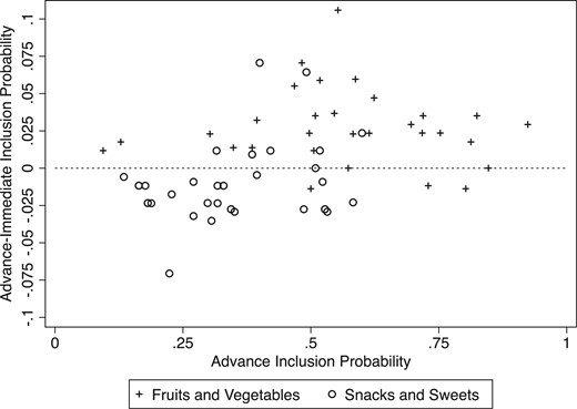
Advance and immediate choice behaviour

Notes: Each point represents the probability with which each food is included in subjects’ bundles over all in a location-week. This makes 60 points in total—30 fruits and vegetables and 30 sweets and salty snacks. Foods appearing more frequently in advance versus immediate bundles lie above the horizontal line. Of the 30 fruits and vegetables, 27 are included with lower probability in immediate choice. Of the 30 sweets and salty snacks, 23 are included with higher probability in immediate choice.

A clear pattern emerges from Figure 2. Fruits and vegetables are chosen with greater likelihood in advance bundles, but inconsistencies for these foods lead to reductions in their inclusion in immediate bundles. Of 30 fruits and vegetables, 27 have higher inclusion probabilities in advance choice relative to immediate choice. Of 30 sweets and salty snacks, 23 have lower inclusion probabilities in advance choice relative to immediate choice. These patterns of inconsistency towards sweets and salty snacks in immediate choice are also prevalent at the individual level. Of the 203 inconsistencies noted above, 112 (55%) alter the proportion of the bundle allocated to fruits and vegetables versus sweets and salty snacks. Of these, 96 of 112 (86%) decrease the proportion of fruits and vegetables in the immediate bundle relative to the advance bundle. Supplementary Figure A1 provides additional analysis with individual measures for bundle calories, and total fat, carbohydrate, and protein across advance and immediate choice. Advance bundles carry more fruits, fewer calories, less fat, fewer carbohydrates, and less protein than immediate bundles.

The systematic patterns of inconsistencies noted above are supported by the statistics in Table 2. For each subject at each point in time, we aggregate bundle characteristics by summing over the chosen foods along observable and nutritional characteristics. We estimate differences between advance and immediate choice using ordinary least squares (OLS) estimation with standard errors clustered at the individual level. We observe significant differences between advance and immediate bundles in almost every nutritional category at both study sites. Inconsistent subjects substitute lower calorie, lower fat, and lower carbohydrate foods with higher calorie, higher fat, and higher carbohydrate foods. These patterns largely come from exchanging fruits and vegetables for sweets and salty snacks.

Table 2

Bundle characteristics

	(1)	(2)	(3)	(4)	(5)	(6)	(7)
	Fruits/Veg	Sweets	Salty snacks	Calories	Fat (g)	Carb (g)	Protein (g)
Panel A: Chicago Study
Immediate choice	−0.220***	0.161***	0.060**	61.573***	4.051***	5.661***	0.338**
	(0.034)	(0.029)	(0.024)	(12.429)	(0.716)	(1.856)	(0.148)
Constant	5.390***	2.628***	1.968***	2,723.890***	89.658***	462.236***	39.414***
	(0.140)	(0.103)	(0.078)	(40.233)	(2.783)	(5.129)	(0.444)
No. of observations	436	436	436	436	436	436	436
No. of subjects	218	218	218	218	218	218	218
Panel B: Los Angeles Study
Immediate choice	−0.168***	0.141***	0.027	57.686**	3.263**	6.254	1.092**
	(0.042)	(0.039)	(0.031)	(25.598)	(1.359)	(3.825)	(0.473)
Constant	6.745***	2.263***	0.986***	3,354.537***	67.616***	665.328***	55.596***
	(0.116)	(0.099)	(0.060)	(60.199)	(3.155)	(8.921)	(1.071)
No. of observations	512	512	512	512	512	512	512
No. of subjects	171	171	171	171	171	171	171
Week control	Yes	Yes	Yes	Yes	Yes	Yes	Yes
Panel C: Pooled Data
Immediate choice	−0.192***	0.150***	0.042**	59.474***	3.626***	5.981***	0.745***
	(0.028)	(0.025)	(0.020)	(14.932)	(0.803)	(2.231)	(0.265)
Constant	6.757***	2.258***	0.979***	3,353.643***	67.435***	665.464***	55.769***
	(0.116)	(0.098)	(0.060)	(59.508)	(3.119)	(8.803)	(1.064)
No. of observations	948	948	948	948	948	948	948
No. of subjects	389	389	389	389	389	389	389
Week control	Yes	Yes	Yes	Yes	Yes	Yes	Yes
Location control	Yes	Yes	Yes	Yes	Yes	Yes	Yes

Notes: Ordinary least squares regression. Dependent variable reported for each column. Standard errors clustered on individual level in parentheses. Levels of significance: *0.10, **0.05, ***0.01.

3.1.2. Commitment demand

Our design elicits commitment demand in the form of giving up the option to exchange foods for the next delivery date. Of 218 subjects in Chicago, 73 (33.5%) demand commitment for their second delivery. In Los Angeles, commitment demand is more frequent than in Chicago. Of 171 subjects in Los Angeles, 134 (78.4%) ever demand commitment, with 69 of 86 (80.2%) doing so in Week 2 and 127 of 171 (74.3%) doing so in Week 3. A potential reason for the difference across study sites is that we offered commitment to Chicago subjects a few days prior to the next delivery, while we offered commitment to Los Angeles subjects immediately after they made their advance choices for the next delivery. However, differences in the sample population and study design across sites make it difficult to identify the underlying reason for this difference.

Figure 3 displays the association between dynamic inconsistency and subsequent commitment demand. In Chicago, 55 of 136 (40.4%) dynamically consistent subjects demand commitment, while only 18 of 82 (22.0%) dynamically inconsistent subjects do so. In Los Angeles, 95 of 105 (90.5%) of subjects who are dynamically consistent in their first delivery ever demand commitment, while only 39 of 66 (59.1%) dynamically inconsistent subjects do so. Of 256 total allocations made in Los Angeles prior to being offered commitment, 123 of 135 (91.1%) dynamically consistent observations and only 69 of 121 (57.0%) dynamically inconsistent observations are linked to any subsequent commitment demand. The correlation between commitment demand and dynamic inconsistency at both study sites is negative and statistically significant at conventional levels—|$\rho = -0.19 ~(p < 0.01)$| in Chicago, and |$\rho = -0.37 ~(p < 0.01)$|⁠, |$\rho = -0.39 ~(p < 0.01)$| in Los Angeles for inconsistency at the first delivery and overall, respectively. Hence, though levels of commitment differ across study sites, the negative relationship between commitment demand and prior inconsistency is reproduced at both locations.

Figure 3

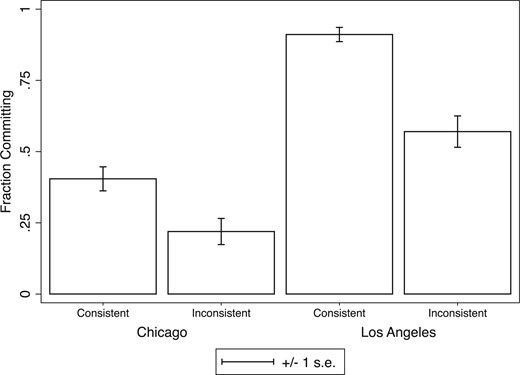
Fraction of committing subjects by prior inconsistency

Notes: This figure displays the fraction of participants who demand commitment, split by whether they were previously dynamically inconsistent.

Table 3 displays OLS regressions on bundle characteristics for committing and non-committing subjects in advance and immediate choice for all allocations made prior to commitment being offered. At both study sites, committing subjects exhibit different behaviour in both advance and immediate choice. Though more pronounced in Los Angeles, committing subjects construct advance bundles with more fruits and vegetables, fewer sweets and salty snacks, and fewer calories. Non-committing subjects exhibit substantial inconsistencies along these dimensions, exchanging fruits and vegetables for sweets and salty snacks. As shown by the interaction terms, committing subjects carry inconsistencies of smaller magnitude, in line with the correlations noted previously.

Table 3

Prior bundle characteristics and commitment demand

	(1)	(2)	(3)	(4)	(5)	(6)	(7)
	Fruits/Veg	Sweets	Salty snacks	Calories	Fat (g)	Carb (g)	Protein (g)
Panel A: Chicago Study
Immediate choice	−0.290***	0.207***	0.083**	80.200***	5.491***	6.722***	0.333
	(0.044)	(0.039)	(0.033)	(16.773)	(0.933)	(2.517)	(0.206)
Committer	0.444	−0.368*	−0.116	−54.762	−9.502	11.149	−1.168
	(0.288)	(0.205)	(0.163)	(85.118)	(5.914)	(10.540)	(0.974)
Immediate |$\times$| Committer	0.207***	−0.138***	−0.069	−55.625**	−4.300***	−3.170	0.017
	(0.064)	(0.053)	(0.045)	(22.953)	(1.365)	(3.481)	(0.267)
Constant	5.241***	2.752***	2.007***	2,742.228***	92.840***	458.503***	39.806***
	(0.175)	(0.133)	(0.096)	(49.544)	(3.378)	(6.473)	(0.522)
No. of observations	436	436	436	436	436	436	436
No. of subjects	218	218	218	218	218	218	218
Panel B: Los Angeles Study
Immediate choice	−0.281**	0.297***	−0.016	108.238	7.522*	6.921	3.124**
	(0.129)	(0.111)	(0.093)	(72.759)	(3.897)	(10.999)	(1.276)
Committer	0.774**	−0.657**	−0.121	−280.291*	−16.782*	−24.072	−5.461**
	(0.310)	(0.255)	(0.135)	(150.516)	(8.587)	(19.605)	(2.753)
Immediate |$\times$| Committer	0.151	−0.208*	0.057	−67.403	−5.678	−0.890	−2.710**
	(0.134)	(0.117)	(0.097)	(76.501)	(4.086)	(11.559)	(1.349)
Constant	6.136***	2.782***	1.080***	3,575.314***	80.862***	684.206***	59.920***
	(0.275)	(0.231)	(0.116)	(130.723)	(7.400)	(17.506)	(2.400)
No. of observations	512	512	512	512	512	512	512
No. of subjects	171	171	171	171	171	171	171
Week control	Yes	Yes	Yes	Yes	Yes	Yes	Yes
Panel C: Pooled Data
Immediate choice	−0.287***	0.234***	0.053	88.786***	6.113***	6.783*	1.187***
	(0.050)	(0.043)	(0.037)	(25.162)	(1.359)	(3.784)	(0.437)
Committer	0.612***	−0.522***	−0.113	−170.697*	−13.365**	−6.557	−3.559**
	(0.211)	(0.163)	(0.106)	(86.895)	(5.223)	(11.116)	(1.483)
Immediate |$\times$| Committer	0.170***	−0.151***	−0.019	−52.430*	−4.449***	−1.435	−0.791
	(0.058)	(0.052)	(0.043)	(30.711)	(1.646)	(4.621)	(0.542)
Constant	6.258***	2.684***	1.069***	3,493.293***	78.407***	670.763***	58.647***
	(0.205)	(0.166)	(0.099)	(89.460)	(5.149)	(12.133)	(1.590)
No. of observations	948	948	948	948	948	948	948
No. of subjects	389	389	389	389	389	389	389
Week control	Yes	Yes	Yes	Yes	Yes	Yes	Yes
Location control	Yes	Yes	Yes	Yes	Yes	Yes	Yes

Notes: Ordinary least squares regression. Standard errors clustered on individual level in parentheses. Levels of significance: *0.10, **0.05, ***0.01.

The reduced form findings in both our Chicago and Los Angeles study sites indicate clear patterns of dynamic inconsistency along with demand for commitment that is negatively correlated with prior inconsistencies. These core facts are consistent with the existence of self-control problems, but indicate that those with the largest problems are systematically less aware thereof. In the next section, we estimate the degree of dynamic inconsistency in food preferences and provide statistical tests for the likelihood that observed behaviour could be delivered by decision makers with consistent preferences. We then use the estimated preferences and the documented correlation between commitment demand and dynamic inconsistency to assess the welfare value of commitment policies and their behavioural effects.

3.2. Structural evidence: dynamically inconsistent preferences and policy evaluation

In Section 2.4, we introduced a random utility model which interprets a given food’s inclusion in the bundle as being driven by a set of food characteristics and random shocks. This links food choices at each point in time, summarized by the advance and immediate orderings, |$r_A$| and |$r_I$|⁠, to utility parameters, |$\beta_A$| and |$\beta_I$|⁠. Table 4 provides structural estimates for each study site. We assume that observable characteristics, such as being a fruit or vegetable and being perishable, and nutritional characteristics, such as grams of fat, carbohydrates, and protein, are potential utility drivers.²³ We stack all orderings obtained when commitment is not available and estimate |$\beta_A$| and |$\beta_I$| simultaneously following the likelihood established in equation (1). Standard errors are clustered by individual.

Table 4

Utility estimates

	(1)	(2)	(3)	(4)	(5)	(6)
	All subjects			Inconsistent subjects
	Chicago	Los Angeles	Pooled	Chicago	Los Angeles	Pooled
Fruit/Vegetable	0.043	0.509***	0.229***	0.064	0.447***	0.217***
	(0.048)	(0.039)	(0.028)	(0.084)	(0.055)	(0.041)
Perishable		0.301***			0.259***
		(0.027)			(0.036)
Fat	−0.007***	0.003*	−0.004***	−0.007*	0.002	−0.005***
	(0.002)	(0.001)	(0.001)	(0.004)	(0.002)	(0.001)
Carbohydrates	0.001**	0.003***	0.002***	0.000	0.003***	0.002***
	(0.000)	(0.000)	(0.000)	(0.001)	(0.000)	(0.000)
Protein	0.031***	−0.023***	−0.001	0.037***	−0.023***	0.000
	(0.006)	(0.004)	(0.003)	(0.010)	(0.006)	(0.004)
Immediate choice
|$\times$| Fruit/Vegetable	−0.072***	−0.063***	−0.050***	−0.200***	−0.131***	−0.117***
	(0.015)	(0.012)	(0.008)	(0.036)	(0.025)	(0.017)
|$\times$| Perishable		−0.025**			−0.052**
		(0.010)			(0.022)
|$\times$| Fat	−0.001	−0.001	0.000	−0.002	−0.002	0.001
	(0.001)	(0.001)	(0.000)	(0.002)	(0.001)	(0.001)
|$\times$| Carbohydrates	0.001***	−0.000	−0.000	0.001***	−0.001	−0.000
	(0.000)	(0.000)	(0.000)	(0.000)	(0.000)	(0.000)
|$\times$| Protein	−0.004	0.003	−0.001	−0.012	0.007	−0.002
	(0.003)	(0.002)	(0.001)	(0.008)	(0.004)	(0.003)
No. of observations	8,720	10,240	18,960	3,280	4,840	8,120
No. of rankings	436	512	948	164	242	406
No. of clusters	218	171	389	82	95	177
Log-likelihood	−18,437.60	−21,343.79	−39,949.47	−6,934.57	−10,128.41	−17,121.39
|$H_0$|⁠: Dynamic consistency	|$\chi^2(4)= 47.63$|	|$\chi^2(5)= 28.54$|	|$\chi^2(4)= 67.89$|	|$\chi^2(4)= 73.33$|	|$\chi^2(5)= 33.95$|	|$\chi^2(4)= 85.43$|
	|$(p < 0.01)$|	|$(p < 0.01)$|	|$(p < 0.01)$|	|$(p < 0.01)$|	|$(p < 0.01)$|	|$(p < 0.01)$|

Notes: Rank Order Logit regression results. Standard errors clustered on individual level in parentheses. Week and location controls are not included given the formulation of covariates as utility drivers. Calories not included as a utility driver as they are collinear with nutritional characteristics. Levels of significance: *0.10, **0.05, ***0.01. Null hypothesis tests stationarity of preferences from interacted rank order Logit regression of choices on nutritional characteristics with different coefficients for immediate choice. Test corresponds to all interaction terms being equal to zero.

We estimate preferences for Chicago subjects in column (1), preferences for Los Angeles subjects in column (2), and preferences in the pooled data in column (3). Results are remarkably similar across study sites. The vector of advance utility weights, |$\beta_A$|⁠, shows significant effects of food characteristics on a food’s value. Controlling for nutritional characteristics, a food being a fruit or vegetable increases its advance value. Interaction effects identify whether food characteristics are weighed differently in immediate choice, estimating the difference between |$\beta_A$| and |$\beta_I$|⁠. Echoing the reduced form evidence on inconsistencies, the utility weight of fruits and vegetables decreases significantly—by around 25%—from advance to immediate choice in the pooled data. Importantly, as can be seen from column (2), which uses Los Angeles data and incorporates perishability, inconsistencies do not appear to be driven by perishability. Perishable items receive lower weight under |$\beta_I$| than |$\beta_A$|⁠, but accounting for perishability doesn’t alter the conclusions drawn with respect to the lower value of fruits and vegetables in immediate choice. These results help to ensure that the possible spoilage of foods does not drive aggregate results of dynamic inconsistency. The hypothesis test of dynamic consistency, |$\beta_A = \beta_I$|⁠, which corresponds to a test of all interaction terms being equal to zero, is rejected at all conventional levels—|$\chi^2(4) = 47.63, ~ (p < 0.01)$| in Chicago and |$\chi^2(4) = 28.54, ~ (p < 0.01)$| in Los Angeles. At the aggregate level, we reject the null hypothesis that the observed differences in choice between advance and immediate conditions could be delivered by dynamically consistent food preferences with random utility shocks.

Columns (4) through (6) of Table 4 repeat the structural analysis for the subgroup of inconsistent subjects (203 of 474 allocation observations and 177 of 389 total subjects). Though inconsistent subjects are remarkably similar to the full sample in terms of advance preferences, immediate preferences show stark reductions in the value of fruits and vegetables. Relative to advance preferences, the utility weight of fruits and vegetables declines by around 50% for inconsistent subjects.²⁴

The models estimated in Table 4 link utility weights for food characteristics to inclusion in the advance and immediate bundles. An evaluation of in-sample model fit is provided in Figure 4. In order to predict the probability with which a given food, |$j$|⁠, will be included in the advance or immediate bundle, we calculate the deterministic portion of the food’s value in advance choice and immediate choice, |${\bf x}_j \beta_A$| and |${\bf x}_j \beta_I$|⁠, under the utility estimates of Table 4, columns (1) and (2). While it is simple to rank the foods according to this deterministic measure, identifying the probability a given food will be included in the bundle is more challenging. The probability that a given food, |$j$|⁠, will be preferred to alternatives |$1, ...,J-K-1$| at a given choice, |$T$|⁠, is calculated analytically as

$$\begin{equation*} F_j[x_1, ..., x_{J-K-1}, x_j; \beta_{T}] = {{\rm{exp}}({\bf x}_j \beta_T) \over {\rm{exp}}({\bf x}_j \beta_T) + \sum_{i=1}^{J-K-1} {\rm{exp}}({\bf x}_i\beta_T) }; ~T\in~ \lbrace A, I \rbrace. \end{equation*}$$

Figure 4

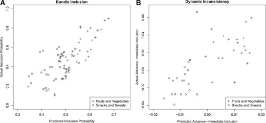
Predicted and actual behaviour

Notes: Panel A: Each point represents the predicted and actual probability with which each food is included in subjects’ bundles over all in a location in either advance or immediate choice prior to commitment being offered. This makes 80 points in total—10 fruits and vegetables and 10 sweets and salty snacks in each location in advance and immediate choice. Predictions generated from 10 million simulations of inclusion probability for each food in each location in each time frame. Correlation in Panel A: |$\rho = 0.73$|⁠. Panel B: Each point represents the predicted and actual difference in inclusion probability between advance and immediate choice in each location. This makes 40 points in total—10 fruits and vegetables and 10 sweets and salty snacks in each location. Correlation in Panel B: |$\rho = 0.73$|⁠.

However, if there are 10 unchosen foods—which is the case for the majority of observations—and 19 alternative foods in total, there are |${19}\choose{10}$|= 92,378 such probabilities to calculate for each food. We opt instead to simulate this inclusion probability by drawing a vector, |${\bf \epsilon}$|⁠, of 20 type 1 extreme value shocks, calculating total utility |${\bf x}_j \beta_T + \epsilon_j$|⁠, and examining whether a given food is ranked in the top 10 of the 20 foods. We draw 10 million |${\bf \epsilon}$| vectors in each location in advance and immediate choice to calculate inclusion probabilities based on the utility estimates of Table 4, columns (1) and (2). Figure 4A graphs this predicted inclusion probability against actual behaviour.²⁵ Notable from Figure 6A is the close correspondence between predicted and actual behaviour, both across the broad categorization of fruit/vegetable versus salty/sweet snack and within them. Overall, the correlation between predicted and actual behaviour is |$\rho =0.73$|⁠. Figure 4B presents predicted and actual differences in inclusion probabilities to assess our model’s ability to match dynamic inconsistency in food choice. There, as well, we find a tight correlation between predicted and actual behaviour both across and within food categories with an overall correlation of |$\rho =0.72$|⁠. Figure 4 demonstrates the quality of our estimated utility model in matching both the level of behaviour and the nature of dynamic inconsistencies in food choice.

3.2.1. Individual welfare consequences of inconsistency

Table 4 and Figure 4 indicate systematic dynamic inconsistencies in food preferences at the aggregate level, which closely correspond to reduced form inconsistencies in food choice. In order to understand the individual welfare consequences of dynamic inconsistency and evaluate the effects of commitment policy, we estimate equation (1) at the individual level using the advance and immediate orderings, |$r_{A,i}, ~r_{I,i}$|⁠.²⁶ Every allocation is considered in isolation, such that subjects who make two allocation decisions in the Los Angeles study site will have two values of |$r_{A,i}$| and |$r_{I,i}$|⁠. The individual rank order logit follows the form of Table 3, column (6) with “Fruit/Vegetable,” “Fat,” “Carbohydrates,” and “Protein” as utility drivers. From this, we construct individual measures of utility and the welfare consequences of any dynamic inconsistency.

Figure 5A provides histograms of |$V_{A,i}({\bf q_{A,i}}) - V_{A,i}({\bf q_{I,i}})\over |V_{A,i}({\bf q_{A,i}})|$| and |$V_{I,i}({\bf q_{A,i}}) - V_{I,i}({\bf q_{I,i}})\over |V_{I,i}({\bf q_{A,i}})|$|⁠, the individual advance and immediate welfare consequences of dynamic inconsistency, for the 203 (of 474 total) inconsistent observations.²⁷ There is wide heterogeneity both between and within welfare measures for the consequences of dynamic inconsistency. Under advance preferences, |$V_{A,i}({\bf q_{A,i}}) - V_{A,i}({\bf q_{I,i}})\over |V_{A,i}({\bf q_{A,i}})|$| has a median [25th–75th percentile] value of 0.044 [|$-$|0.031, 0.146]. Under immediate preferences, |$V_{I,i}({\bf q_{A,i}}) - V_{I,i}({\bf q_{I,i}})\over |V_{I,i}({\bf q_{A,i}})|$| has a median [25th–75th percentile] value of |$-$|0.055 [|$-$|0.169, 0.026]. The median disagreement between advance and immediate preferences is intuitive: advance preferences suggest costs to inconsistency and immediate preferences suggest benefits to flexibility. Indeed, there is broad distributional disagreement in the advance and immediate welfare measures, with greater costs to inconsistency under the advance welfare measure and greater benefits to flexibility under the immediate measure, Mann–Whitney |$z= 10.13,~(p < 0.01)$|⁠. In Supplementary Figure A2, we present the same analysis measuring the welfare consequences of inconsistency in terms of “best-food” equivalents rather than as a proportion of total utility, and find qualitatively similar results.

Figure 5

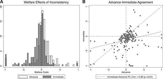
Advance and immediate welfare consequences of dynamic inconsistency

Notes: Panel A provides a histogram of individual estimates of the welfare costs of inconsistency under advance and immediate preferences. Panel B provides a scatterplot of agreement between advance and immediate welfare measures for the inconsistent observations. Panel B points graphed with 10% jitter.

Figure 5B relates advance and immediate welfare measures for the inconsistent observations. Though this relationship generally falls below the 45|$^{\circ}$| line of perfect agreement, a significant correlation does exist, |$\rho = 0.28,~ (p < 0.01)$|⁠. The line of best fit highlights the general pattern of disagreement, with immediate welfare measures tending to suggest more benefits to flexibility than advance measures. Sixty-eight of 203 individual observations (33.5%) exhibit disagreement in sign between advance and immediate measures. All but 1 of these 68 disagreements are in the direction of the medians, with 67 observations having |${V_{A,i}({\bf q_{A,i}}) - V_{A,i}({\bf q_{I,i}})\over |V_{A,i}({\bf q_{A,i}}) |}> 0 $| and |${V_{I,i}({\bf q_{A,i}}) - V_{I,i}({\bf q_{I,i}})\over |V_{I,i}({\bf q_{A,i}})| }< 0$|⁠. The welfare measures for the remaining 135 observations agree in sign, with 69 (34.0%) exhibiting unanimous costs to dynamic inconsistency, and 66 (32.5%) exhibiting unanimous benefits to flexibility.²⁸

The advance and immediate utility measures yield intuitive results for the welfare effects of dynamic inconsistency: advance utility suggests median costs to inconsistency while immediate utility suggests median benefits to flexibility. Where disagreements in the consequences of dynamic inconsistency exist, they may be helpfully arbitrated by the unambiguous utility estimates, |$\beta_U$|⁠, estimated from the unambiguous ordering, |$r_U$|⁠.²⁹ Figure 6A presents the individual unambiguous welfare measure, |${V_{U,i}({\bf q_{A,i}}) - V_{U,i}({\bf q_{I,i}})\over |V_{U,i}({\bf q_{A,i}})| }$|⁠, constructed from the unambiguous orderings, |$r_{U,i}$|⁠. The unambiguous welfare measure has median [25th–75th percentile] value of 0.003 [|$-$|0.106, 0.107], with 102 of 203 (50.3%) observations exhibiting unambiguous welfare costs to inconsistency. When advance and immediate welfare measures agree, so too does the unambiguous measure with all 135 values of |${V_{U,i}({\bf q_{A,i}}) - V_{U,i}({\bf q_{I,i}})\over |V_{U,i}({\bf q_{A,i}})| }$| sharing the same sign. When the advance and immediate welfare measures disagree, 34 of 68 (50%) have values of |${V_{U,i}({\bf q_{A,i}}) - V_{U,i}({\bf q_{I,i}})\over |V_{U,i}({\bf q_{A,i}}) |}> 0$|⁠, implying welfare costs to inconsistency.

Figure 6

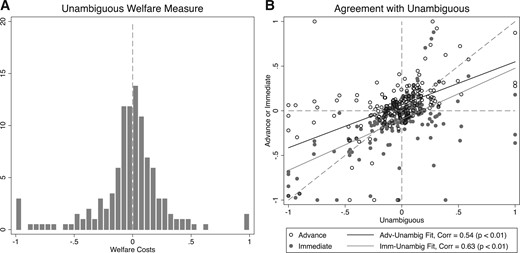
Unambiguous welfare consequences of dynamic inconsistency

Notes: Panel A provides a histogram of individual estimates of the welfare costs of inconsistency under unambiguous preferences. Panel B provides a scatterplot of agreement between unambiguous and advance or immediate welfare measures. Panel B points graphed with 10% jitter.

Figure 6B relates the unambiguous to the advance and immediate welfare measures. Both the advance and immediate welfare measures are substantially more correlated with the unambiguous measure than they are with each other, |$\rho = 0.54~ (p < 0.01)$| and |$\rho = 0.63~ (p < 0.01)$|⁠, respectively. These patterns of connection are also intuitive: though disagreement exists between advance and immediate orderings, their commonalities are respected by the unambiguous ordering, and hence, the unambiguous welfare measure. Further, the lines of best fit highlight the general tendency of advance measures to exceed, and immediate measures to fall below, the unambiguous welfare consequences of inconsistency.

3.2.2. Commitment policy evaluation

The reduced form results demonstrate that dynamically inconsistent subjects are less likely to take up commitment than are dynamically consistent subjects. This basic correlation along with the clear patterns of inconsistency towards less healthy food items suggest that those with the largest self-control problems are the least aware thereof. A negative correlation between inconsistency and awareness generates the potential for quite limited effects of policies which simply offer commitment. If such policies are taken up by those who experience the smallest self-control problems, then muted behavioural and welfare effects (regardless of utility measure) should be expected. All non-committing and all dynamically consistent individuals are unaffected by the policy and these make up the overwhelming majority, 387 of 474 (81.6%), of our observations. This is despite the fact that 207 of 389 subjects (53.2%) ever demand commitment. We examine the effects of our implemented commitment policy along both the behavioural and welfare dimensions.

We evaluate the predicted behavioural consequences of offering commitment using the correlation noted above between inconsistencies and any subsequent commitment demand, and the decisions individuals made prior to commitment being offered. For individuals who ultimately chose not to commit, we consider the characteristics of their immediate bundles prior to commitment being offered. For individuals who ultimately chose to commit, we consider the characteristics of their advance bundles prior to commitment being offered. These bundles are contrasted in percentage terms with those actually chosen by all subjects (i.e. their immediate bundle) to develop a predicted effect of the program. Table 5 carries the corresponding results. We predict that offering commitment would have quite limited effects, generating around 1% more fruits and vegetables and about 2% fewer sweets.

Table 5

Behavioural policy evaluation (predicted and actual)

	(1)	(2)	(3)	(4)	(5)	(6)	(7)
	Fruits/Veg	Sweets	Salty snacks	Calories	Fat (g)	Carb (g)	Protein (g)
Offer commitment—predicted	1.1%	−1.8%	−1.3%	−0.6%	−1.1%	−0.5%	−0.4%
	(0.3)	(0.6)	(0.8)	(0.3)	(0.6)	(0.3)	(0.4)
Offer commitment—artefactual	0.7%	−2.0%	0.4%	−0.2%	−0.6%	−0.1%	−0.1%
	(0.5)	(1.3)	(2.7)	(0.6)	(1.4)	(0.4)	(0.6)
Offer commitment—	6.0%	−8.7%	−11.9%	−9.2%	−17.2%	−6.9%	−6.7%
experimental (LA)
	(4.3)	(7.5)	(12.7)	(3.5)	(8.1)	(2.6)	(4.1)

Notes: Evaluation of policy offering commitment. Predicted values generated by considering only choices made prior to commitment being offered, comparing decisions actually made in immediate choice with those implied by restricting to advance choice for the subset of subjects who ultimately chose commitment. Artefactual values generated by augmenting analysis of Table 2 with final week of data. Experimental values generated by focusing only on immediate choice in Los Angeles in Week 2 of the study where commitment was offered at random. Supplementary Table A4 provides regression results.

The second row of Table 5 also provides estimates of the actual effect of offering commitment by augmenting the prior data of Table 2 with the final week of decisions in which commitment was offered and examining the interaction effect between immediate choice and commitment offer (expressed as a percent). Commitment has virtually no effect on the extent of inconsistencies in bundle characteristics, closely in line with the predicted values. The final row of Table 5 provides the same analysis but focuses only on immediate choice in the second week in Los Angeles, where commitment was offered experimentally. These experimental results suggest larger effects of the policy but are estimated with substantial imprecision. Effects for observable characteristics such as being a fruit or vegetable are not distinguishable from zero, while effects for the nutritional characteristics of fat and carbohydrates (and hence calories) do reach statistical significance.³⁰

We predict the welfare effects of offering commitment by contrasting the costs of dynamic inconsistency through the lens of the individual preference measures, |$\beta_{A,i}$|⁠, |$\beta_{I,i}$|⁠, and |$\beta_{U,i}$|⁠, captured prior to commitment being offered. Specifically, we evaluate the proportion of observations where costs of inconsistency—e.g.|${ V_{A,i}({\bf q}_{A,i}) - V_{A,i}({\bf q}_{I,i}) \over |V_{A,i}({\bf q}_{A,i}) |}$| for advance utility—are predicted to increase, decrease, or remain constant under the policy relative to complete flexibility.

All non-committing and dynamically consistent individuals are predicted to be unaffected by the commitment offer. Given that 87 of 474 (18.4%) observations are both dynamically inconsistent and associated with subsequent commitment, offering commitment is unsurprisingly predicted to affect a minority of individuals. Under the most favourable welfare criterion, the advance measure, only 59 of 474 (12.5%) observations would see welfare improvements from commitment, while 28 (5.9%) would see welfare reductions.³¹ Under the immediate measure, 34 of 474 (7.2%) observations would see welfare improvements and 53 of 474 (11.2%) would see reductions. Under the unambiguous measure, 46 of 474 (9.7%) observations would see welfare improvements and 41 of 474 (8.7%) would see reductions. Ultimately, the limited behavioural effects of offering commitment are mirrored closely in the limited welfare consequences of the policy. Simply offering commitment doesn’t alter behaviour on aggregate and doesn’t affect any but the slim minority of individuals with both self-control problems and awareness.

3.2.3. Alternate policies

The analysis to here suggests that commitment policies as traditionally implemented will likely have limited behavioural and welfare consequences (regardless of the utility measure). In Table 6 and Figure 7, we contrast the impacts of the standard policy to two alternatives: mandating advance choice for all subjects; and a tailored mandate, requiring advance choice only for a specific subset of individuals based on whether they are predicted to have unambiguous welfare costs to dynamic inconsistency, |${ V_{U,i}({\bf q}_{A,i}) - V_{U,i}({\bf q}_{I,i}) \over |V_{U,i}({\bf q}_{A,i})|} > 0 $|⁠.³² Mandating advance choice leads to around three times larger behavioural effects than offering commitment—3% more fruits and vegetables and 6% fewer sweets than no policy—but has the potential for substantially negative welfare consequences. The policy affects the 203 of 474 (42.8%) inconsistent observations. Under the advance welfare measure, 136 of 474 observations (28.7%) are made better off and 67 (14.1%) are made worse off. Under the immediate welfare measure, 70 of 474 observations (14.8%) are made better off and 133 (28.1%) are made worse off. Under the unambiguous welfare measure, 102 of 474 observations (21.5%) are made better off and 101 (21.3%) are made worse off.

Table 6

Alternate policy evaluation—predicted behavioural effects

	(1)	(2)	(3)	(4)	(5)	(6)	(7)
	Fruits/Veg	Sweets	Salty snacks	Calories	Fat (g)	Carb (g)	Protein (g)
Offer commitment (predicted)	1.1%	−1.8%	−1.3%	−0.6%	−1.1%	−0.5%	−0.4%
	(0.3)	(0.6)	(0.8)	(0.3)	(0.6)	(0.3)	(0.4)
Mandate advance choice (predicted)	3.2%	−6.0%	−2.9%	−1.9%	−4.6%	−1.0%	−1.5%
	(0.5)	(1.0)	(1.4)	(0.5)	(1.0)	(0.4)	(0.5)
Tailored mandate (predicted)	1.9%	−3.1%	−2.5%	−0.7%	−2.7%	0.1%	−0.9%
	(0.3)	(0.7)	(1.0)	(0.3)	(0.7)	(0.3)	(0.3)

Notes: Evaluation of policy offering commitment. Predicted values for commitment generated by considering only choices made prior to commitment being offered, comparing decisions actually made in immediate choice with those implied by restricting to advance choice for the subset of subjects who ultimately chose commitment. Predicted values for mandated advance choice generated by considering only choices made prior to commitment being offered, comparing decisions actually made in immediate choice with those implied by restricting all subjects to advance choice. Predicted values for tailored mandate generated by considering only choices made prior to commitment being offered, comparing decisions actually made in immediate choice with those implied by restricting to advance choice for the subset of individuals with |${V_{U,i}({\bf q}_{A,i}) - V_{U,i}({\bf q}_{I,i}) \over |V_{U,i}({\bf q}_{A,i})|} > 0$|⁠.

Figure 7

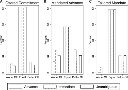
Alternate policy evaluation—predicted welfare effects

Notes: This figure summarizes the percentage of individuals who are predicted to be worse, equal, or better off under advance, immediate, and unambiguous welfare criteria for each policy. Panel A displays the policy of simply offering commitment, Panel B displays the policy of mandated advance choice, and Panel C displays the policy of a tailored mandate.

The tailored mandated has intermediate behavioural effects, generating 2% more fruits and vegetables and 3% fewer sweets than without intervention. The policy affects 102 of 474 (21.5%) observations, making it similarly impactful in percentage terms to offering commitment. Under this policy, no subjects can be worse off according to the unambiguous measure, and all 102 (21.5%) observations with |${ V_{U,i}({\bf q}_{A,i}) - V_{U,i}({\bf q}_{I,i}) \over |V_{U,i}({\bf q}_{A,i})|} > 0 $| are made better off. Under the advance measure, 101 of 474 observations (21.3%) are made better off, and 1 (0.2%) is made worse off. Under the immediate measure 69 of 474 observations (14.6%) are made better off, and 33 (7%) are made worse off. The tailored policy carries potential benefits over simply offering commitment or mandating advance choice for all. The proportion of better off (worse off) individuals greater (lower) than that of offering commitment, and the relative proportion of winners to losers is greater regardless of the preference measure. Relative to mandated advance choice for all, the tailored mandate dramatically reduces the proportion of individuals who are negatively affected by the policy, while maintaining a sizable proportion of beneficiaries. Such a policy may be of potential interest for future research in this area given these characteristics.

3.3. Robustness tests and additional exercises

Our exercise interprets dynamically inconsistent behaviour as evidence of dynamically inconsistent preferences. Though our structural exercise examines the possibility that inconsistent behaviour exists with consistent preferences, this is done through the lens of the model. In this subsection, we provide additional evidence that dynamic inconsistency is a product of preferences rather than an alternate force such as the resolution of uncertainty, changing environmental factors or noise. We also evaluate the stability of inconsistency and commitment along with providing an additional exploration of complementarities and non-linearities in food preferences.

3.3.1. “Want” versus “should” foods

Models of dynamically inconsistent preferences are often organized around a narrative of temptation. There are foods decision-makers should be consuming and those that they want to consume. In our Los Angeles study site, we provided subjects with two forms of food rating data. In the first, subjects were asked how much they liked eating the food, including aspects such as how the food tastes.³³ We term this the “want” ranking. In the second, subjects were asked how often they felt they should eat each food.³⁴ We term this the “should” ranking.

Table 7 follows the structural exercise from actual food choices to contrast the preferences implied by the “want” and “should” rankings. Column (1) shows differences between “want” and “should” preferences in line with choices. Fruits and vegetables are valued according to “should” preferences, but receive lower weight in “want” preferences. In column (2), we restrict attention to the 125 Los Angeles subjects who provided both “want” and “should” rankings for all foods and find similar results. In columns (3)–(6), we examine differences in “want” and “should” preferences by commitment choice and dynamic inconsistency. Interestingly, individuals who are inconsistent and individuals who do not commit have smaller percentage differences in their “want” and “should” preferences for fruits and vegetables than those who are consistent and those who demand commitment. These data are in line with the interpretation that those with larger self-control problems are less aware thereof and hence are less likely to commit.

Table 7

“Want” versus ‘should” utility estimates in Los Angeles Study

	(1)	(2)	(3)	(4)	(5)	(6)
	All subjects	Complete rankings
			|${\rm Inconsistent} = 0$|	|${\rm Inconsistent} = 1$|	|${\rm Commit} = 0$|	|${\rm Commit} = 1$|
Fruit/Vegetable	1.708***	1.705***	1.730***	1.684***	1.573***	1.745***
	(0.077)	(0.090)	(0.130)	(0.126)	(0.218)	(0.099)
Perishable	0.987***	0.961***	0.989***	0.937***	0.814***	1.004***
	(0.059)	(0.068)	(0.099)	(0.094)	(0.156)	(0.075)
Fat	0.003*	0.001	0.003	0.000	0.002	0.001
	(0.002)	(0.002)	(0.003)	(0.003)	(0.005)	(0.002)
Carbohydrates	0.004***	0.004***	0.004***	0.004***	0.003**	0.005***
	(0.000)	(0.001)	(0.001)	(0.001)	(0.001)	(0.001)
Protein	−0.036***	−0.032***	−0.037***	−0.029***	−0.018	−0.036***
	(0.005)	(0.006)	(0.008)	(0.009)	(0.015)	(0.007)
Want ranking
|$\times$| Fruit/Vegetable	−0.735***	−0.749***	−0.675***	−0.805***	−0.770***	-0.739***
	(0.093)	(0.108)	(0.160)	(0.147)	(0.254)	(0.120)
|$\times$| Perishable	−0.207***	−0.174**	−0.108	−0.227**	−0.291*	−0.147*
	(0.066)	(0.077)	(0.105)	(0.110)	(0.173)	(0.087)
|$\times$| Fat	−0.007***	−0.007***	−0.004	−0.010**	−0.019***	−0.004
	(0.002)	(0.003)	(0.004)	(0.004)	(0.007)	(0.003)
|$\times$| Carbohydrates	−0.000	−0.000	0.000	−0.000	−0.001	−0.000
	(0.001)	(0.001)	(0.001)	(0.001)	(0.002)	(0.001)
|$\times$| Protein	0.018***	0.017**	0.006	0.026**	0.050***	0.009
	(0.007)	(0.008)	(0.013)	(0.010)	(0.016)	(0.009)
No. of observations	6,550	5,000	2,280	2,720	1,000	4,000
No. of rankings	331	250	114	136	50	200
No. of clusters	171	125	57	68	25	100
Log-likelihood	−12,551.59	−9,602.47	−4,360.75	−5,238.58	−1,952.41	−7,639.93
|$H_0$|⁠: Want = Should	|$\chi^2(5)= 71.13$|	|$\chi^2(5)= 57.27$|	|$\chi^2(5)= 23.29$|	|$\chi^2(5)= 36.82$|	|$\chi^2(5)= 19.79$|	|$\chi^2(5)= 44.58$|
	|$(p < 0.01)$|	|$(p < 0.01)$|	|$(p < 0.01)$|	|$(p < 0.01)$|	|$(p < 0.01)$|	|$(p < 0.01)$|

Notes: Rank Order Logit regression results. Standard errors clustered on individual level in parentheses. Levels of significance: *0.10, **0.05, ***0.01. The “want” rating was provided on a 1–7 scale from “Dislike Very Much” to “Like Very Much.” The “should” rating was provided on a 1–5 scale from “Never’‘ to “Every Day.” Null hypothesis tests equality of “want” and “should” preferences from interacted rank order logit regression of choices on nutritional characteristics with different coefficients for “want” rankings. Test corresponds to all interaction terms being equal to zero.

3.3.2. Stability of inconsistency and commitment

Our data demonstrate evidence of dynamic inconsistency when comparing advance and immediate decisions. Though the data patterns are indicative of a change in preference rather than shocks, specific forms of resolution of uncertainty may lead to apparent time inconsistencies. For example, perishable foods such as fruits and vegetables may appear less attractive than packaged foods such as sweets and salty snacks on the day of delivery. The foods in our Los Angeles study were chosen with this critique in mind. The similarity in results between Chicago and Los Angeles helps alleviate this concern.

Additional exercises can be taken to ensure that observed dynamic inconsistencies are not simply driven by changes in environmental factors. First, we can examine whether individuals who are inconsistent at one delivery remain so at future deliveries. Of our 389 subjects, 182 never chose commitment. For these subjects, the correlation between inconsistency before and after commitment is offered is |$\rho = 0.33,~(p <0.01)$|⁠. This positive association through time suggests some stability at the individual level. Additionally, 85 subjects in Los Angeles made two allocation decisions prior to being offered commitment. For these subjects the correlation in dynamic inconsistency over the 2 weeks is |$\rho = 0.20,~ (p = 0.07)$|⁠. This lower correlation is driven by a growing tendency of inconsistency over the 2 weeks: 28 of 34 individuals were inconsistent in the first week were again inconsistent, but 29 of 51 individuals who were not inconsistent in the first week became inconsistent.

Second, we can examine whether changes in the decision environment relate to observed inconsistencies. For example, for people with children, decisions may be made with or without children present. For 343 of our 389 subjects, we have a survey response to their total number of children. Ninety of 343 (26%) report having no children. The correlation between having no children and dynamic inconsistency prior to commitment is |$\rho = -0.05,~(p = 0.38)$|⁠, indicating that those less likely to experience the environmental change of having children present during the decision are no more or less likely to exhibit inconsistencies. Further, in Los Angeles, our study staff recorded the number of children present at registration at first delivery for all 171 subjects. The correlation between having more kids present at delivery than registration and dynamic inconsistency is |$\rho = 0.03~(p = 0.67)$|⁠.

Another possible source of environmental change is the decision maker’s current level of hunger. In our Los Angeles study, 170 of 171 subjects rated their current hunger level on a 4-point scale from “Very Hungry” to “Not At All Hungry” both at registration and delivery. The correlation between changing one’s report to “Very Hungry” from a lower hunger level and dynamic inconsistency is |$\rho = 0.07~(p = 0.37)$|⁠. Additionally, in our Los Angeles study, we used a series of questions to measure food security—i.e. levels of access to food due to lack of resources—at registration and delivery (Blumberg et al., 1999). The correlation between growing more food insecure from registration to delivery and dynamic inconsistency is |$\rho = 0.003~(p = 0.97)$|⁠.

A final potential change to the decision environment is the resources available to the decision maker. In our Los Angeles study, subjects who receive monthly SNAP benefits were asked about their remaining SNAP dollar balance at both registration and delivery. Fifty-seven of 171 Los Angeles subjects provided these reports, and having less available balance at delivery than registration is actually negatively correlated with dynamic inconsistency, though not significantly so, |$\rho = -0.19~(p = 0.17)$|⁠. Taken together, these findings indicate that observable changes in decision environment are unlikely to drive our observed inconsistencies.

Our Los Angeles data also allow us to examine the stability of commitment demand. Eighty-six of our 171 Los Angeles participants were asked if they desired commitment for both their second and third delivery. The correlation between demanding commitment across these two deliveries is |$\rho = 0.46~(p <0.01)$|⁠. Of the 69 subjects who demanded commitment for their second delivery, 61 subsequently demanded commitment for their third delivery. This gives further indication of commitment as a deliberate choice taken by a set of subjects who have relatively small self-control problems.

3.3.3. Complementarities and non-linearities in food preferences

Our structural analysis estimating dynamically inconsistent preferences linked bundle inclusion for a given good to its observable and nutritional characteristics. This effectively posits bundle inclusion as a linear function of own good characteristics. Two implicit assumptions may be worthy of further consideration. First, though in practice individuals generally only placed one of each chosen item in their bundle, they could choose to add more. Apparently the number of current units in the bundle deeply affects the value of adding more, such that utility of a given good may be non-linear in its chosen quantity. Food-specific marginal utility must drop quite quickly to generate the diversity of bundles we observe in practice. Second, individuals may also wish to construct diverse bundles because perhaps fruits and vegetables are complementary to sweets and salty snacks in consumption.

Abstracting from rapidly diminishing food-specific utilities—an issue which actually helps to justify our exercise estimating inclusion rather than quantity—one could employ an alternate strategy which broadly considers diminishing marginal utility for fruits and vegetables and sweets and salty snacks, along with complementarities across these two observable characteristics. One benefit of focusing on these observable characteristics as the central utility drivers is that our experiment is well-founded as a convex budget over these two dimensions with a price ratio of 1. Let |$f$| indicate fruits and vegetables and |$s$| indicate snacks or sweets. Our experiment asks subjects to solve the following problem

$$\begin{equation*} \max_{f,s}~ U(f,s) ~ s.t. ~ f + s = M,\end{equation*}$$

with |$M= 10$| foods. As in all other structural exercises, we can make functional form assumptions to yield estimates of key parameters of interest. For example, under Cobb–Douglas preferences, |$U(f,s) = f^\alpha s^{1-\alpha}$|⁠, the marginal condition yields

$$\begin{eqnarray*} \alpha = \frac{1}{{s\over f} +1}.\end{eqnarray*}$$

The fraction of unhealthy to healthy goods identifies the key utility parameter, |$\alpha$|⁠. Utility parameter |$\alpha$| in hand, one further obtains solution functions |$f^*(M) = \alpha M$|⁠, |$s^*(M) = (1-\alpha) M$|⁠, and indirect utility function |$U(M) = U(f^*(M), s^*(M)) = [\alpha^\alpha (1-\alpha)^{1-\alpha}] M$|⁠.

Let |$(f_A, s_A)$| represent the choice in advance choice with corresponding utility |$U_A(f_A, s_A)$| parameterized by |$\alpha_A$|⁠. Let |$(f_I, s_I)$|⁠, |$U_I(f_I, s_I)$|⁠, and |$\alpha_I$| represent similar values in immediate choice. The utility parameter is well defined for allocations |$(f, s)$| away from the corner solutions, |$s/f = 0$| and |$s/f = \infty$|⁠, a condition which is satisfied for 194 of our 203 inconsistent observations. The median [25th–75th percentile] value of |$\alpha_A$| implied by choice |$(f_A, s_A)$| is 0.6 [0.5, 0.7]. The median [25th–75th percentile] value of |$\alpha_I$| implied by choice |$(f_I, s_I)$| is 0.5 [0.4, 0.7].

We create measures of equivalent variation by identifying the value |$M'$| at which the agent is indifferent between the change in decision timing and maintaining the same time frame and altering the number of foods to choose. For advance choice, this equivalent variation, |$EV_A = M- M'_A$|⁠, is identified from |$U_A(M'_A) = U_A(f^*_I(M), s^*_I(M))$|⁠. For immediate choice, this equivalent variation, |$EV_I = M- M'_I$|⁠, is identified from |$U_I(M'_I) = U_I(f^*_A(M), s^*_A(M))$|⁠. The median [25th–75th percentile] value of |$EV_A$| is 0.20 [0, 0.22] foods. The median [25th–75th percentile] value of |$EV_I$| is also 0.20 [0, 0.22].

According to advance preferences, the equivalent variation of allowing immediate choice is around 0.2 or 2% fewer foods. Similarly, according to immediate preferences, the equivalent variation of restricting to advance choice is around 0.2 or 2% fewer foods. These percentage differences are in the same range as those calculated at the individual level presented in Figure 5. Correspondence in the nature and level of welfare consequences across measurement techniques indicates robustness to the various welfare conclusions drawn in our exercise.

4. Discussion and Conclusion

In two field experiments, we provide evidence on dynamic inconsistency and commitment demand in food choice. We show that dynamic inconsistencies are prevalent, with over 40% of subjects exhibiting inconsistency in choice. The direction of inconsistency is systematically towards less healthy foods: compared to advance choice, immediate choice decreases the amount of fruits and vegetables selected and increases calories and fat content. Using structural estimation, we find welfare effects of dynamic inconsistency on the order of around 5% of total utility, with the direction of the effect depending on the welfare criterion used.

We also find substantial demand for commitment, with over half of subjects voluntarily restricting themselves to their advance choice. Importantly, we document a negative correlation between dynamic inconsistency and subsequent commitment demand. This suggests that those with the largest self-control problems may lack sufficient awareness to demand commitment.

Our results contrast with prior studies which find a weak positive correlation between commitment demand and present bias. Since our negative correlation is observed in both of our experiments, we believe it is unlikely to be due to chance alone. Instead, it is possible that the different results between our work and prior work are due to the context (we study food choice, other studies focus on other environments), or due to the fact that our study is conducted in a more natural environment, wherein subjects were not told that they were under observation. Existing puzzles related to commitment demand in field settings may benefit from a deeper understanding of this correlation, with our findings providing one key observation.

Interestingly, at both study sites, subjects who demand commitment also make more healthy advance decisions even when commitment is not available. This result resonates with one recent finding on commitment demand in gym attendance by Royer et al. (2015), who find greater commitment demand among subjects who are already exercising regularly. These findings suggest that those whose behaviour (and welfare) would be most affected by commitment may be the least likely to take it up. More research is needed in field environments to understand the nuanced relationship between preferences, dynamic inconsistency, and awareness.

Our research is critical for understanding the behavioural impacts and welfare consequences of commitment policies. In our studies, we use individuals’ advance choices, immediate choices, and unambiguous choices to evaluate the behavioural and welfare consequences of various policies. An important application is comparing a policy that offers commitment to a policy that mandates advance choice for a subset of individuals with unambiguous costs to inconsistency. A common concern with mandated advance choice is that while it may have large effects on behaviour, it may reduce welfare compared to offering commitment. Our welfare analysis in this context is perhaps surprising. We find that offering commitment does little to change behaviour or improve welfare, with those who benefit from the program roughly equalling those who lose depending on the welfare measure. However, a tailored policy of mandated advance choice would increase healthy choices while maintaining a distribution of welfare consequences tilted towards those who benefit from the program under all welfare measures.

It is also important to recognize that the specific commitment device we offer restricts choice for a single week in the future. Commitment devices such as penalized withdrawals on retirement savings often commit individuals in multiple future periods. Such devices differ in two important ways. First, the potential welfare consequences could be substantially larger as each period in which immediate and advance preferences differ will have utility consequences. Second, the disagreement between different welfare measures on the value of commitment may be substantially decreased. The intuitive logic is that advance and immediate preferences disagree immediately but agree for future dates. In addition to understanding commitment values for longer-term commitments, it will be important for future work to investigate the core relationship between dynamic inconsistency and take-up of long-term commitment devices.

Finally, our results give insights to innovations in food policy. For example, our results add to our understanding of the impact of a policy change now under consideration at the USDA that would allow pre-ordering under SNAP. Our study provides an understanding of how this policy change would affect the food choice and welfare of consumers. Our study can also help guide how to craft those policies in ways that both achieve greater behavioural change and align policy goals closely with concerns for individual welfare.

The editor in charge of this paper was Nicola Gennaioli.

Acknowledgments.

This project was funded by a grant from the USDA BECR center, a USDA Cooperative agreement, grant #G-2015-14107 from the Alfred P. Sloan Foundation and generous donations from the Understanding America Study (UAS) panel members at USC. We thank Terri Zhu at Louis’ Groceries and Teresa Blanco at Northgate Gonzalez Market for helping us in the field. For helpful comments, we thank Stefano DellaVigna, David Laibson, and numerous seminar and conference participants. We thank Andre Gray, Dustin Pashouwer and undergraduate students at the Behavioral and Experimental Economics research group for research assistance. This research was conducted with IRB approval from the University of Wisconsin-Madison and the University of Southern California. The content of this paper is solely the responsibility of the authors and does not necessarily represent the official views of the funding sources or the UAS.

Footnotes

1.

Importantly, Laibson (2015) notes alternative rationales for the low level of commitment demand, including environmental uncertainty and costs of commitment. As such, commitment demand may be limited even among agents who are aware of their self-control problems. Sadoff and Samek (2018) explore interventions to increase commitment demand in the context of food choice.

2.

John (2018) also shows that take-up of an un-windable commitment device is negatively correlated with the interaction of her two measures, consistent with sophisticated present-biased individuals having a better forecast on high default probabilities within the commitment device. In experimental settings, dynamic inconsistency can explain only about 5% of the variation in commitment demand (Augenblick et al., 2015) and individuals seem to understand less than 25% of their self-control problems (Augenblick and Rabin, 2018).

3.

Our treatment of unambiguous choices differs in one critical way from the Bernheim and Rangel (2007, 2009) approach. Our noted utility model estimates utility weights based on the choices subjects make, either advance choices, immediate choices, or the intersection thereof, unambiguous choices. The Bernheim and Rangel (2007, 2009) approach would take the unambiguous choice relation and derive non-parametric welfare measures therefrom. These measures would never contradict choices made in advance or immediate conditions and would, hence, be unable to arbitrate between inconsistent choices. Using the unambiguous choice relation to estimate utility weights allows one to construct a utility value for every food, including foods that were exchanged between advance and immediate conditions. The unambiguous utility will thus arbitrate an inconsistency and can potentially contradict advance or immediate choice. This deviation, along with our general practice of filtering choices through a utility model to provide our welfare estimates, has costs and benefits that are discussed in detail in Section 2.4.2.

4.

In Section 3.3.3, we explore an alternate estimation strategy without this feature, considering choice of bundle composition, and find quite similar results.

5.

This compares favourably to simply offering commitment, a policy which we predict generates more worse off individuals: 5.9% under the advance measure, 9.7% under the unambiguous measure, and 11.2% under the immediate measure.

6.

Related studies include Duflo et al. (2011) for farmer fertilizer purchase; Augenblick et al. (2015) for effort choices in a laboratory experiment; and subsequent to our study, Augenblick and Rabin (2018) also for effort choices in the laboratory.

7.

A food desert is defined as having a poverty rate of 20% or greater and at least 33% of the census tract lives more than one mile from a supermarket or large grocery store (http://apps.ams.usda.gov/fooddeserts/fooddeserts.aspx).

8.

See https://www.cdc.gov/obesity/data/adult.html.

9.

See https://www.fns.usda.gov/snap/online-purchasing-pilot.

10.

Four hundred and ten subjects were initially recruited into the study. Of these 410, 21 (5.12%) are considered attrited from the study due to not completing the full set of deliveries (17), never being offered a commitment decision due to experimenter error (3), or opting out after the study ended (1).

11.

According to the 2010 U.S. Census, Greater Grand Crossing has a population of 35,217, the majority of whom are African Americans (97.8%). South-Central Los Angeles has a population of 169,453. The majority of residents are Hispanic (74%) and African-American (24%). A larger share of our LA study participants were Hispanic (98%), since the store caters to Hispanic customers. Both neighbourhoods have high rates of poverty (28.5–33.6%).

12.

In the Chicago experiment, The University of Wisconsin-Madison Institutional Review Board (IRB) required us to notify subjects after the study was complete that they had participated and give them the option to withdraw their data. One subject chose to withdraw, and this subject’s data are not in the dataset. The Los Angeles experiment was approved by the University of Southern California’s IRB, which did not have this requirement.

13.

In Chicago, the question was worded as, Please tell us how much you like the following foods, where 1 is DO NOT LIKE AT ALL and 7 is LIKE VERY MUCH. The question was worded slightly differently in Los Angeles. It was, For foods that you have eaten, I’d like to know how much you like eating the food. When you answer how much you like eating the food, please think carefully about how much you enjoy the food, including aspects such as how the food tastes to you. [point to food] How much do you like eating the food? Do you not like it at all, do not like it, do not like it a little, have no preference, like it a little, like it or like it very much?

14.

Completing a rating for all foods was voluntary; nevertheless, most subjects rated a large number of foods, with 357 of 389 (92%) rating 15 or more foods. In Chicago 191 of 218, or 88% rated at least 15 foods. In Los Angeles 166 of 171, or 97% rated at least 15 foods. This difference could be because in Chicago, subjects wrote down their responses while in Los Angeles, subjects responded verbally.

15.

In Los Angeles, the message was slightly different, Here is your food delivery [show box]. Please take a look [bring open basket, allow person to look through]. We also have some extra items available. If you like, you can exchange any one item in your basket for one of these items [show extra items in tray]. I brought all the menu items, and you can make up to 4 exchanges. Do you want to make any exchange? [Great thanks, let me note that on your order sheet].

16.

A similar arbitrage argument is used to question the use of monetary payments in studies of intertemporal choice (Cubitt and Read, 2007; Chabris et al., 2008; Andreoni and Sprenger, 2012; Augenblick et al., 2015).

17.

Or, alternatively, that subjects construed the task as choosing their 10 favourite foods, ignoring a portion of our instructions.

18.

Eighty-five percent of fruits and vegetables are reported to be consumed within 1–3 days, compared to 84% of sweets and salty snacks (Fisher’s exact |$p = 0.67$|⁠). Eighty-five percent of perishable items are reported to be consumed within 1–3 days, compared to 84% for non-perishable items (Fisher’s exact |$p = 0.59$|⁠).

19.

To address these concerns, Toussaert (2015) elicits beliefs about the behaviour of similar others rather than oneself. However, de Oliveira and Jacobson (2017) demonstrate that people may have systematically different beliefs about their own time preferences versus those of others.

20.

An alternative structural methodology is to consider each bundle of 10 items as a potential option and consider the discrete choice problem of picking the best bundle. With 20 foods, there are |${20}\choose{10}$|= 184,756 possible bundles of 10 unique items, and |${20 + 10 - 1}\choose{10}$| = 20,030,010 possible bundles of 10 items with repetitions. For both tractability and interpretability, we opt to formulate food and bundle utilities as being derived from a set of characteristics. Note, however, that our construction is not able to capture, for example, a preference for diversity in the bundle or complementarities between items. We explore complementarities explicitly in Section 3.3.3 using an alternate estimating strategy that focuses on bundle composition, rather than each food’s inclusion.

21.

Note that the intensive margin of choice represented by the quantities |${\bf q}$| is not a feature of the estimated likelihood, but is present in the determination of utility values. Given that most chosen bundles consist of only unique food items, the distinction between the extensive and intensive margin is rarely of importance in our setting.

22.

In the second week of study in our Los Angeles study site, 85 subjects made allocations without commitment being offered. Of these, 57 (67%) were inconsistent. This proportional increase in inconsistency relative to the first week is driven primarily by individuals who were previously consistent becoming inconsistent (29 of 51 (57%) previously consistent subjects). Among the 34 previously inconsistent subjects, 28 (82%) were again inconsistent in the second week. Though a correlation does exist in inconsistency over time, we were unable to uncover any clear predictors for this changing level of behaviour through time. Section 3.3.2 provides additional exploration of stability of both inconsistency and commitment demand in our studies.

23.

Calories are not included as a utility driver as they are collinear with nutritional characteristics. There are 9 calories in 1 fat gram, 4 calories in 1 carbohydrate gram, and 4 calories in 1 protein gram. Hence, calories = 9*Fat (g) + 4*Carb (g) + 4*Protein (g).

24.

Supplementary Table A3 provides structural estimates separately for committing and non-committing subjects. Echoing the reduced form results, committing subjects exhibit advance preferences that are more favourable to fruits and vegetables, and smaller changes in estimated preferences moving from advance to immediate choice.

25.

Because the estimation of Table 4, column (2) is conducted without week controls for Los Angeles, we predict inclusion probabilities in Los Angeles for all observations without commitment offered and contrast it with the actual behaviour. Hence, Figure 4 has 40 observations in advance and immediate choice rather than the 60 in Figure 2.

26.

Beggs et al. (1981) also provide individual estimates for stated preferences over electric cars and compare individual and aggregate results.

27.

Naturally, the relevant value for the 271 dynamically consistent individuals will be zero. The absolute value of the denominator is used because a small proportion of observations have estimated utility parameters that imply negative bundle values. Twenty-nine of 203 (14.3%) inconsistent observations have |$V_{A,i}({\bf q_{A,i}}) <0 $|⁠, and 45 of 203 (22%) inconsistent observations have |$V_{I,i}({\bf q_{A,i}}) < 0$|⁠. The absolute value ensures that we correctly capture the direction of change for our proportional measure. The utility measures are top and bottom-coded at |$\pm1$|⁠.

28.

Recall that such agreement is a feature of our estimation exercise which calculates food values based from estimated attribute utility weights informed by all choices at a given point in time. As such, inconsistencies may be viewed as increasing or decreasing the total bundle value from both the advance and immediate perspective.

29.

Aggregate estimates for |$\beta_U$| constructed by eliminating exchanged foods are provided in Supplementary Table A2.

30.

The larger point estimates are due to the notably high level of inconsistency among individual who were not offered commitment. Nonetheless, the likely negative contemporaneous correlation between potential inconsistency and take-up of commitment leaves the effects statistically imprecise. Supplementary Table A4 provides the regression estimates behind the analysis of Table 5, rows 2 and 3.

31.

Note that these calculations do not incorporate actual choices made when commitment is offered.

32.

Of 474 observations, 102 (21.5%) have |${ V_{U,i}({\bf q}_{A,i}) - V_{U,i}({\bf q}_{I,i}) \over |V_{U,i}({\bf q}_{A,i})|} > 0 $| and so would have their advance choice mandated, while 372 (80%) have |${ V_{U,i}({\bf q}_{A,i}) - V_{U,i}({\bf q}_{I,i}) \over |V_{U,i}({\bf q}_{A,i})|} \le 0 $| and would have flexibility mandated. In effect, this policy honours the unambiguous preferences, |$\beta_{U,i}$|⁠, and tailors contract terms depending on whether dynamic inconsistencies are estimated to be detrimental or beneficial.

33.

This rating was provided on a 1–7 scale from “Dislike Very Much” to “Like Very Much.”

34.

This rating was provided on a 1–5 scale from “Never” to “Every Day.”